Introduction: The Power of Motor Imagery and the Rise of EEG-Based BCIs
Brain-Computer Interfaces (BCIs) have emerged as a groundbreaking technology, transforming the way humans interact with machines. From medical rehabilitation to entertainment , BCIs are redefining human-machine interaction. Among the various BCI paradigms, Motor Imagery (MI) has gained significant traction due to its ability to activate the sensorimotor cortex—similar to real movement (RM) and motor observation (MO) —without actual physical movement.
However, most existing research focuses on upper limb MI classification, with limited exploration of lower limb MI, especially for separate left and right limb classification. This is where the MSC-T3AM Transformer model comes into play—a novel deep learning architecture that leverages multi-scale separable convolutional attention and knowledge distillation (KD) to achieve superior classification accuracy in multi-action lower limb MI tasks .
In this article, we’ll explore how the MSC-T3AM model improves EEG signal classification , how knowledge distillation enhances performance, and why this breakthrough matters for future BCI applications .
Understanding the Challenge: Why Lower Limb MI Classification is Hard
The Limitations of Traditional EEG Classification Models
Traditional methods such as Common Spatial Patterns (CSP) , Filter Bank CSP (FBCSP) , and Support Vector Machines (SVMs) have been widely used for EEG classification. However, these techniques suffer from several limitations:
- Manual feature engineering limits adaptability.
- Inability to capture global features from EEG signals.
- Poor generalization across different subjects and motor tasks.
- Limited attention to multiple EEG signal dimensions (e.g., spatial, temporal, and spectral).
Deep learning models like Convolutional Neural Networks (CNNs) and Recurrent Neural Networks (RNNs) have improved classification performance. However, they still struggle with:
- Capturing long-term dependencies (RNNs).
- Modeling global spatial-temporal patterns (CNNs).
- High computational cost and memory consumption (especially with Transformers).
The MSC-T3AM Solution: A Transformer-Based 3D-Attention Framework
What is MSC-T3AM?
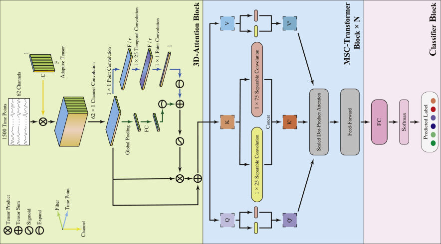
MSC-T3AM stands for Multi-Scale Separable Convolutional Transformer-based Filter-Spatial-Temporal Attention Model . It’s designed to classify six types of lower limb motor actions :
- Motor Imagery (MI) – Left and Right
- Real Movement (RM) – Left and Right
- Motor Observation (MO) – Left and Right
The model integrates three key components :
- 3D-Attention Block
- MSC-Transformer Blocks
- Classifier Block with Knowledge Distillation
Let’s break down each component.
1. The 3D-Attention Block: Extracting Local Features Across Dimensions
Why 3D Attention?
EEG signals are inherently multi-dimensional , containing spatial , temporal , and spectral information. Traditional models often treat these dimensions separately, leading to information loss .
The 3D-Attention Block addresses this by applying attention mechanisms across:
- Spatial Attention Module
- Filter Attention Module
- Temporal Attention Module
Each module dynamically adjusts the weight of features along its respective dimension, ensuring that the model focuses on the most relevant EEG features .
Spatial Attention Module
- Applies spatial convolution to emphasize brain regions associated with motor activity.
- Helps identify the central and midline regions of the brain—critical for lower limb control.
Filter Attention Module
- Uses global average pooling to compute filter weights .
- Highlights the most informative frequency bands for MI classification.
Temporal Attention Module
- Extracts local temporal features using point convolution and temporal convolution .
- Enhances the model’s ability to capture EEG dynamics over time.
2. The MSC-Transformer Blocks: Capturing Global Features Efficiently
Why Use a Transformer?
Transformers excel at modeling long-range dependencies and global patterns —ideal for EEG signals, which are non-stationary and complex .
However, standard Transformers suffer from high computational complexity , especially with long EEG sequences .
How MSC Improves Transformer Efficiency
The Multi-Scale Separable Convolution (MSC) is applied after the query, key, and value projections in the self-attention module. This reduces computational load while improving classification accuracy .
- Multi-scale kernels (e.g., (1×25), (1×75)) capture both short-term and long-term temporal patterns .
- Depth-wise separable convolutions reduce model parameters without sacrificing performance.
3. Knowledge Distillation: Learning from Implicit Information
What is Knowledge Distillation (KD)?
Knowledge Distillation (KD) allows a smaller model (student) to learn from a larger, pre-trained model (teacher) . It leverages the probability distribution of the teacher model’s outputs—implicit knowledge that traditional methods ignore.
Why Use KD in MSC-T3AM?
- Improves classification accuracy by learning inter-class relationships .
- Reduces model size while maintaining performance.
- Enhances robustness to EEG signal variability .
Offline vs. Online KD
| TYPE | DESCRIPTION | ADVANTAGES |
|---|---|---|
| Offline KD | Teacher model is pre-trained; student learns from it during training. | Faster training; stable teacher model. |
| Online KD | Teacher and student models are trainedsimultaneously. | Dynamic learning; adapts to new data. |
Results show that online KD outperforms offline KD in classification accuracy by 2%–19% .
Performance Evaluation: How MSC-T3AM Stands Out
Dataset and Experimental Setup
The model was tested on a dataset containing 28 subjects , each performing 6 motor actions (MI-L, MI-R, RM-L, RM-R, MO-L, MO-R), with 72 trials per action .
- 62 EEG channels + 2 EOG channels
- Sampling rate : 250 Hz
- Frequency band : 8–30 Hz
Comparison with State-of-the-Art Models
| MODEL | MEAN ACCURACY | F1-SCORE | KAPPA |
|---|---|---|---|
| EEGNet | 46.23% | 0.4608 | 0.3547 |
| ATCNet | 43.81% | 0.4369 | 0.3258 |
| DeepConvNet | 43.43% | 0.4337 | 0.3212 |
| FBCSP-SVM | 42.73% | 0.4261 | 0.3117 |
| MSC-T3AM (Online KD) | 48.41% | 0.4825 | 0.3810 |
Key Findings
- MSC-T3AM with online KD achieved the highest classification accuracy .
- Filter and Temporal Attention Modules contributed the most to performance (2.8% improvement).
- Spatial Attention and MSC Module added 1.2% and 1% respectively.
Ablation Study: The Impact of Each Module
| MODULES INCLUDED | ACCURACY |
|---|---|
| None | 39.44% |
| Spatial Attention | 43.45% |
| Filter + Temporal | 44.13% |
| MSC Module | 41.38% |
| Filter + Temporal + MSC | 46.41% |
| Spatial + MSC | 44.62% |
| Spatial + Filter + Temporal | 46.29% |
| All Modules | 47.44% |
This ablation study confirms that multi-dimensional attention and multi-scale convolution are essential for high-performance EEG classification .
Feature Visualization: Understanding the Brain Regions Involved
Event-Related Desynchronization (ERD) and Synchronization (ERS)
ERD/ERS patterns were visualized to identify brain regions activated during different motor tasks.
- RM tasks activated frontal regions .
- MO tasks activated occipital regions .
- MI tasks activated central regions —consistent with motor cortex activity.
Topographic Maps of Attention Weights
The spatial attention module of MSC-T3AM with online KD focused heavily on the central and midline regions —areas responsible for lower limb motor control .
This visualization confirms that the model is interpretable and aligns with neuroscientific findings .
Mathematical Formulation: The Science Behind MSC-T3AM
Loss Function with Knowledge Distillation
The student model is optimized using a combination of Cross-Entropy (CE) loss and Kullback-Leibler (KL) divergence loss :
$$ L = \alpha L_{\text{CE}} + (1 – \alpha) L_{\text{KL}} $$
Where:
$$L_{\text{CE}}(p, y) = -\sum_{i=1}^{n} y_i \log(p(x_i))$$
$$L_{\text{KL}}(p_s, p_t) = \sum_{i=1}^{n} p_t\left(\frac{x_i}{T’}\right) \log\left( \frac{p_t\left(\frac{x_i}{T’}\right)}{p_s\left(\frac{x_i}{T’}\right)} \right)$$
- pt : softened probability vector of the teacher model
- ps : softened probability vector of the student model
- T′ : temperature hyperparameter
Softmax with Temperature Scaling
$$ p_t(x_i / T’) = \frac{\exp(f_t(x_i)/T’)}{\sum_{j=0}^{n-1} \exp(f_t(x_j)/T’)} $$ $$p_s(x_i / T’) = \log\left( \frac{\exp(f_s(x_i)/T’)}{\sum_{j=0}^{n-1} \exp(f_s(x_j)/T’)} \right)$$This formulation ensures smooth probability distributions , improving model generalization .
If you’re Interested in BAST-Mamba model based on deep learning, you may also find this article helpful: 7 Powerful Reasons BAST-Mamba Is Revolutionizing Binaural Sound Localization — Despite the Challenges
Conclusion: Why MSC-T3AM is a Game-Changer
The MSC-T3AM Transformer model with online knowledge distillation sets a new standard for multi-action lower limb MI classification . Its 3D-attention mechanism , multi-scale convolution , and knowledge distillation framework make it highly accurate , computationally efficient , and interpretable .
Key Advantages of MSC-T3AM
- High classification accuracy (48.41% mean accuracy)
- Robust to EEG signal variability
- Interpretable attention maps
- Efficient model architecture
- Supports real-time BCI applications
Call to Action: Stay Ahead with Cutting-Edge BCI Research
Are you working on EEG-based BCI systems , rehabilitation technologies , or neural signal processing ? Then you can’t afford to miss out on the MSC-T3AM Transformer model .
- Explore the GitHub repository : MSC-T3AM GitHub
- Read the full paper : MSC-T3AM Paper
- Join the BCI revolution —apply this model in your research or applications today!
Final Thoughts: The Future of EEG Classification is Here
As BCIs continue to evolve, models like MSC-T3AM will play a crucial role in enabling more accurate, intuitive, and responsive brain-computer interactions. Whether it’s for medical rehabilitation , gaming , or assistive robotics , the integration of attention mechanisms and knowledge distillation marks a paradigm shift in EEG signal processing.
By leveraging deep learning , Transformer architectures , and knowledge distillation , we’re not just improving classification accuracy—we’re unlocking the full potential of the human brain .
FAQs
1. What is Motor Imagery (MI)?
Motor Imagery refers to the mental rehearsal of a movement without actual physical execution. It activates the sensorimotor cortex , making it ideal for BCI applications.
2. What is Knowledge Distillation (KD)?
KD is a technique where a smaller model (student) learns from a larger, pre-trained model (teacher) by mimicking its output probability distribution.
3. What is the advantage of online KD over offline KD?
Online KD allows simultaneous training of both teacher and student models, enabling dynamic learning and better adaptation to new data.
4. How does MSC-T3AM improve classification accuracy?
Through 3D attention modules , multi-scale separable convolutions , and online knowledge distillation , MSC-T3AM captures multi-dimensional EEG features more effectively.
5. Can I use MSC-T3AM for real-time BCI applications?
Yes. The model is computationally efficient , making it suitable for real-time EEG classification in BCI systems.
Below is a stand-alone, self-contained PyTorch 1.12+ implementation of the model described in the paper “MSC-transformer-based 3D-attention with knowledge distillation for lower-limb EEG classification”.
import torch, torch.nn as nn, torch.nn.functional as F
from einops import rearrange
from torch.utils.data import DataLoader, TensorDataset
import numpy as np

DEVICE = 'cuda' if torch.cuda.is_available() else 'cpu'
T        = 1.5        # temperature for KD
ALPHA    = 0.7        # weight of CE loss in KD
BANDS    = 8          # number of learned frequency filters (F)
CHANNELS = 62         # number of EEG channels   (C)
TIME     = 1500       # number of time points    (T)
N_CLASS  = 6          # six lower-limb actions
3-D Attention Block (Filter × Spatial × Temporal)
class SpatialAttention(nn.Module):
    def __init__(self, C, F):
        super().__init__()
        self.w = nn.Parameter(torch.randn(F, 1, C))  # (F,1,C)

    def forward(self, x):            # x: (B,F,C,T)
        x = x * self.w             # channel-wise re-weight
        return x                   # (B,F,C,T)

class FilterAttention(nn.Module):
    def __init__(self, F, r=2):
        super().__init__()
        self.mlp = nn.Sequential(
            nn.AdaptiveAvgPool3d((F,1,1)),
            nn.Flatten(),
            nn.Linear(F, F//r), nn.ReLU(),
            nn.Linear(F//r, F)
        )

    def forward(self, x):            # x: (B,F,C,T)
        w = self.mlp(x)            # (B,F)
        w = torch.sigmoid(w).unsqueeze(-1).unsqueeze(-1)
        return x * w               # (B,F,C,T)

class TemporalAttention(nn.Module):
    def __init__(self, F, T, r=2, k=25):
        super().__init__()
        self.conv = nn.Sequential(
            nn.Conv2d(F, F//r, 1), nn.ReLU(),
            nn.Conv2d(F//r, F//r, (1,k), padding=(0,k//2)), nn.ReLU(),
            nn.Conv2d(F//r, 1, 1)
        )

    def forward(self, x):            # x: (B,F,C,T)
        # treat (C,T) as H,W of 2-D feature map
        w = self.conv(x.mean(2, keepdim=True))  # (B,1,1,T)
        w = torch.sigmoid(w)
        return x * w               # (B,F,C,T)

class Attention3D(nn.Module):
    def __init__(self, C, F, T):
        super().__init__()
        self.spatial = SpatialAttention(C, F)
        self.filter  = FilterAttention(F)
        self.temp    = TemporalAttention(F, T)

    def forward(self, x):
        x = self.spatial(x)
        x = self.filter(x)
        x = self.temp(x)
        return x
MSC-Transformer Block
class MultiScaleSeparableConv(nn.Module):
    """Depth-wise separable convolutions with two kernel sizes."""
    def __init__(self, F, k_list=[25,75]):
        super().__init__()
        self.convs = nn.ModuleList([
            nn.Sequential(
                nn.Conv2d(F, F, (1,k), groups=F, padding=(0,k//2)),
                nn.Conv2d(F, F, 1)
            ) for k in k_list
        ])

    def forward(self, x):            # x: (B,F,C,T)
        outs = [conv(x) for conv in self.convs]
        return torch.stack(outs, dim=0).mean(0)  # average multi-scale

class MSC_T_Block(nn.Module):
    def __init__(self, F, n_heads=8):
        super().__init__()
        self.F = F
        self.h = n_heads
        self.d_k = F // n_heads
        assert F % n_heads == 0

        self.W_q = nn.Conv2d(F, F, 1)
        self.W_k = nn.Conv2d(F, F, 1)
        self.W_v = nn.Conv2d(F, F, 1)
        self.msc = MultiScaleSeparableConv(F)
        self.ff  = nn.Sequential(nn.Conv2d(F, 4*F, 1), nn.GELU(),
                                 nn.Conv2d(4*F, F, 1))
        self.norm1 = nn.GroupNorm(1, F)
        self.norm2 = nn.GroupNorm(1, F)

    def forward(self, x):            # x: (B,F,C,T)
        B,F,C,T = x.shape
        q = rearrange(self.W_q(x), 'b (h d) c t -> b h (c t) d',
                      h=self.h, d=self.d_k)
        k = rearrange(self.W_k(x), 'b (h d) c t -> b h (c t) d',
                      h=self.h, d=self.d_k)
        v = rearrange(self.W_v(x), 'b (h d) c t -> b h (c t) d',
                      h=self.h, d=self.d_k)

        scores = torch.matmul(q, k.transpose(-2,-1)) / np.sqrt(self.d_k)
        attn   = F.softmax(scores, dim=-1)
        out    = torch.matmul(attn, v)
        out    = rearrange(out, 'b h (c t) d -> b (h d) c t', c=C, t=T)
        out    = self.norm1(x + self.msc(out))
        out    = self.norm2(out + self.ff(out))
        return out
Full Model (MSC-T3AM)
class MSC_T3AM(nn.Module):
    def __init__(self, C=CHANNELS, T=TIME, F=BANDS, n_blocks=3, n_class=N_CLASS):
        super().__init__()
        # Learnable frequency filters (F×1×1 conv on raw 1×C×T)
        self.filter_bank = nn.Conv2d(1, F, (1,1))
        self.att3d   = Attention3D(C, F, T)
        self.blocks  = nn.ModuleList([MSC_T_Block(F) for _ in range(n_blocks)])
        self.pool    = nn.AdaptiveAvgPool2d(1)
        self.classifier = nn.Sequential(
            nn.Flatten(),
            nn.Linear(F, n_class)
        )

    def forward(self, x):            # x: (B,1,C,T)
        x = self.filter_bank(x)      # (B,F,C,T)
        x = self.att3d(x)
        for blk in self.blocks:
            x = blk(x)
        x = self.pool(x).squeeze(-1).squeeze(-1)  # (B,F)
        return self.classifier(x)    # (B,n_class)
class KDLoss(nn.Module):
    def __init__(self, T, alpha):
        super().__init__()
        self.T = T
        self.alpha = alpha
        self.ce = nn.CrossEntropyLoss()
        self.kl = nn.KLDivLoss(reduction='batchmean')

    def forward(self, student_logits, teacher_logits, y_true):
        ce_loss = self.ce(student_logits, y_true)
        soft_teacher = F.log_softmax(teacher_logits / self.T, dim=1)
        soft_student = F.log_softmax(student_logits / self.T, dim=1)
        kl_loss = self.kl(soft_student, soft_teacher) * (self.T ** 2)
        return self.alpha * ce_loss + (1-self.alpha) * kl_loss
def train_one_epoch(net, teacher, loader, opt, criterion):
    net.train()
    if teacher is not None: teacher.eval()
    tot, cor = 0, 0
    for x, y in loader:
        x, y = x.to(DEVICE), y.to(DEVICE)
        logits_s = net(x)
        if teacher is not None:
            with torch.no_grad():
                logits_t = teacher(x)
            loss = criterion(logits_s, logits_t, y)
        else:
            loss = criterion.ce(logits_s, y)
        opt.zero_grad(); loss.backward(); opt.step()
        pred = logits_s.argmax(1)
        cor += (pred == y).sum().item()
        tot += y.size(0)
    return cor / tot
if __name__ == "__main__":
# Synthetic 100 samples, 6 classes
X = torch.randn(100, 1, CHANNELS, TIME)
Y = torch.randint(0, N_CLASS, (100,))
loader = DataLoader(TensorDataset(X,Y), batch_size=16, shuffle=True)
student = MSC_T3AM().to(DEVICE)
teacher = MSC_T3AM().to(DEVICE) # can be any pre-trained CNN (e.g. EEGNet)
opt = torch.optim.Adam(student.parameters(), 1e-3)
criterion = KDLoss(T=T, alpha=ALPHA)
for epoch in range(5):
acc = train_one_epoch(student, teacher, loader, opt, criterion)
print(f"Epoch {epoch+1}: acc={acc:.3f}")