Malaria remains a devastating global health crisis. The World Health Organization’s 2022 report painted a grim picture: 247 million cases and 619,000 deaths. While curable, timely and accurate diagnosis is the critical bottleneck, especially in resource-limited regions where skilled microscopists are scarce and human fatigue leads to errors. The gold standard – microscopic examination of thick blood smears – is notoriously difficult: parasites are tiny, embedded in complex backgrounds filled with noise and artifacts.
Traditional AI approaches, including deep learning models like CNNs and even object detectors (YOLO variants), often stumble. They treat all features equally, ignoring the inherent uncertainty introduced by noisy data. This leads to unstable predictions and missed diagnoses. But a groundbreaking new approach is changing the game: Uncertainty-Guided Attention Learning.
The Thick Smear Challenge: Why Standard AI Falls Short (The Problem)
Thick blood smears offer superior sensitivity for detecting low parasite densities (approximately 11 times higher than thin smears). However, this advantage comes at a cost:
- Tiny Targets: Parasites appear as minuscule purple disks (Fig 1a), often just ~44 pixels in diameter.
- Complex Background: Smears contain distracting elements like white blood cells (WBCs – Fig 1a), staining artifacts, debris, and overlapping cells.
- Noise & Variability: Image quality varies drastically due to staining protocols, slide preparation, and imaging equipment.
- “Candidate” Overload: Automated screening first identifies hundreds/thousands of potential parasite locations (“candidates”) – most are false positives (distractors). Classifying these accurately is the core task.
Standard deep learning models process these candidate patches but lack a mechanism to gauge the reliability of the features they extract from noisy inputs. Unreliable features poison the classification, leading to false negatives (missed parasites) and false positives (wasted resources).
The Revolutionary Solution: Uncertainty-Guided Attention Learning (The 7 Key Breakthroughs)
Researchers from Macquarie University, University of Sydney, and University of Essex introduced a novel neural network architecture that tackles the uncertainty problem head-on. Here are the 7 core breakthroughs:
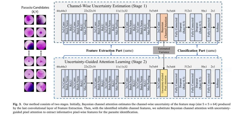
- Bayesian Channel Attention (BCA): Quantifying Feature Uncertainty
Instead of assigning a single importance weight to each feature channel (like standard Channel Attention), BCA reformulates attention under a Bayesian framework. It estimates both the mean importance (μ) and the uncertainty (varianceσ²) for every channel in the feature map derived from the candidate patch.
μ (Mean): Expected importance of the channel’s feature.
σ² (Variance): Uncertainty associated with that importance estimate. High variance = Low reliability.
Input-Adaptive: Uncertainty depends on the specific input patch’s noise level. (Fig 5 shows variability).
Key Innovation: First method to estimate feature map channel uncertainty explicitly for malaria detection.
2. Reliability Weights: Silencing Unreliable Channels
The estimated uncertainty (σ²) is converted into a Reliability Weight (w_σ) for each channel:
$$\mathbf{w}_{\sigma} = \exp(-\beta\sigma^{2}) \quad (\beta > 0 \text{ is a hyperparameter})$$
- Channels with low uncertainty (
σ²small) →wσ≈ 1 (Highly Reliable, fully utilized). - Channels with high uncertainty (
σ²large) →wσ≈ 0 (Unreliable, suppressed).
Effect: Filters out noise and unreliable information before further processing. (See Fig 5 visualization).
3. Uncertainty-Guided Pixel Attention (UGPA): Focusing on Trustworthy Pixels
Traditional Pixel Attention highlights important spatial locations within the feature map. UGPA supercharges this by focusing only on reliable channels:
Breakthrough: Pixel-level focus is now informed by channel-level reliability. UGPA extracts fine-grained spatial details only from trustworthy features.
4. Lightweight & Efficient Two-Stage Architecture
The overall system is pragmatic and deployable:
- Stage 1 (Preselection): Use established methods (e.g., IGMS algorithm) to extract ~300-500 candidate patches per smear image, removing large distractors like WBCs.
- Stage 2 (Classification): The core innovation – A modified VGG19 backbone equipped with BCA and UGPA modules processes each candidate patch.
Computational Feasibility: Only 1.0 Million parameters, ~6-10 Giga FLOPs per image, inference in 0.8-2.1 seconds. (See Table 4).
5. Superior Performance on Real-World Datasets
Tested rigorously on two public, diverse datasets collected under different conditions:
- CMM (Clinical Malaria Microscopy): 239 images, 2986 parasites.
- Thick Smears 150: 1819 images, 84,961 parasites.
Results consistently outperformed 7 state-of-the-art baselines (YOLOv5 variants, PDNet, Transformers – Nest, RegionViT, TransMIL) across parasite-level and patient-level metrics.
Table 1: Performance Dominance on Thick Smears 150 Dataset (Parasite-Level)
| Method | Precision (%) | Recall (%) | F1 Score (%) | AP (%) |
|---|---|---|---|---|
| YOLOv5 | 78.99 | 83.52 | 81.19 | 73.83 |
| YOLOv5opt | 75.84 | 67.41 | 71.38 | 81.67 |
| YOLOv4-Mod | 77.99 | 81.47 | 79.60 | 72.22 |
| PDNet (Previous Best) | 82.19 | 82.74 | 82.46 | 76.65 |
| Proposed (Ours) | 83.15 | 85.13 | 84.13 | 77.77 |
Achieved Highest AP (Critical for Screening): 77.77% (Parasite-Level) and 69.65% (Patient-Level) on Thick Smears 150.
Robust to Small Datasets: Maintained significant lead on smaller CMM dataset where transformers faltered.
Interpretability: Flagging Low-Confidence Predictions
The estimated uncertainty scores (σ²) provide valuable insight:
- Patches dominated by high-uncertainty channels can be flagged for human expert review.
- Enhances trust and allows clinicians to focus efforts where the AI is least confident.
- A crucial step towards reliable human-AI collaboration in diagnostics.
Practical Deployment Potential for High-Throughput Screening
The combination of high accuracy (F1 84.13%), computational efficiency (2.1s/image), and interpretability makes this AI uniquely suited for real-world use:
- Scalable: Processes high-resolution smears efficiently via candidate screening.
- Adaptable: Core concept (uncertainty-guided feature selection) applicable beyond malaria (e.g., other parasite/abnormal cell detection in pathology).
- Addresses Resource Gap: Potential to alleviate burden in under-staffed, malaria-endemic areas.
If you’re Interested in Event-Based Action Recognition based on deep learning, you may also find this article helpful: 7 Revolutionary Ways Event-Based Action Recognition is Changing AI (And Why It’s Not Perfect Yet)
Why This Trumps Other Methods (Including Transformers)
- Object Detection Failures (YOLO etc.): Struggle with tiny parasite size and severe class imbalance in whole high-res images.
- Transformer Limitations: Require massive datasets to avoid overfitting; performance plummeted on the smaller CMM dataset (239 images) compared to CNNs. Also less efficient for small patch inputs.
- Standard Attention Shortcomings: Self-Attention, Channel Attention, Pixel Attention, and Multi-Head Attention all lack explicit uncertainty modeling, making them vulnerable to noisy features. Ablation studies proved UGPA’s superiority (Table 3, Fig 8).
- Pure Uncertainty Methods: Prior work focused on quantifying prediction uncertainty for decisions, not on using feature uncertainty to actively improve feature learning and robustness like UGPA does.
The Path Forward: From Lab to Field
This uncertainty-guided attention approach represents a significant leap forward in automated malaria diagnosis. Its strengths are clear:
- Unprecedented Accuracy: Highest reported AP/F1 scores on benchmark thick smear datasets.
- Built-in Robustness: Explicitly handles data noise and uncertainty at the feature level.
- Clinical Relevance: Provides interpretable confidence measures and operates at practical speeds.
- Generalizable Core: The Bayesian uncertainty + guided attention paradigm holds promise for numerous other medical image analysis tasks suffering from noise and ambiguity.
Call to Action:
- Researchers: Explore integrating this uncertainty-guided attention mechanism into other diagnostic AI models for parasites, cancer cells, or microbiological analysis. Investigate theoretical underpinnings of its robustness.
- Diagnostic Developers & Health Agencies: Prioritize validation and deployment studies of this technology in field settings. Its efficiency and accuracy make it a prime candidate for point-of-care or central lab high-throughput screening systems in malaria-endemic regions.
- Clinicians & Public Health Experts: Engage with AI developers to define requirements and ensure these tools address real-world diagnostic bottlenecks effectively and ethically.
The battle against malaria demands smarter tools. By harnessing the power of uncertainty, not just ignoring it, this AI provides a brighter, more reliable path towards faster diagnosis, effective treatment, and ultimately, saving lives. Let’s move this breakthrough from the pages of research into the clinics where it’s needed most.
Paper Link: Uncertainty-guided attention learning for malaria parasite detection in thick blood smears
Below is a complete, self-contained PyTorch implementation of the Uncertainty-Guided Attention Learning model described in the paper.
# pip install torch==2.1.0 torchvision tqdm
import torch
import torch.nn as nn
import torch.nn.functional as F
from torch import Tensor
from typing import Tuple

class BayesianChannelAttention(nn.Module):
    """
    Channel-wise attention with input-dependent uncertainty.
    Returns:
        attended_feature: Tensor (N, C, H, W)
        channel_sigma:    Tensor (N, C, 1, 1)   (σ²) – uncertainty
    """

    def __init__(self, in_ch: int, prior_precision: float = 1.0):
        super().__init__()
        self.prior_precision = prior_precision
        self.gap = nn.AdaptiveAvgPool2d(1)
        self.fc_mu = nn.Sequential(
            nn.Linear(in_ch, in_ch // 8, bias=False),
            nn.ReLU(inplace=True),
            nn.Linear(in_ch // 8, in_ch, bias=False)
        )
        self.fc_logvar = nn.Sequential(
            nn.Linear(in_ch, in_ch // 8, bias=False),
            nn.ReLU(inplace=True),
            nn.Linear(in_ch // 8, in_ch, bias=False)
        )

    def forward(self, x: Tensor) -> Tuple[Tensor, Tensor]:
        # Global average pooling -> (N,C)
        z = self.gap(x).squeeze(-1).squeeze(-1)
        mu = self.fc_mu(z)
        logvar = self.fc_logvar(z)
        sigma = torch.exp(0.5 * logvar)              # σ
        eps = torch.randn_like(mu)
        z_sample = mu + sigma * eps                  # reparameterization
        attn = torch.sigmoid(z_sample).unsqueeze(-1).unsqueeze(-1)
        attended = x * attn + x                      # residual
        return attended, sigma.unsqueeze(-1).unsqueeze(-1)

class PixelAttention(nn.Module):
    """Plain pixel-wise attention (spatial)."""
    def __init__(self, in_ch: int):
        super().__init__()
        self.conv = nn.Sequential(
            nn.Conv2d(in_ch, in_ch // 8, 1, bias=False),
            nn.ReLU(inplace=True),
            nn.Conv2d(in_ch // 8, 1, 1, bias=False),
            nn.Sigmoid()
        )

    def forward(self, x: Tensor) -> Tensor:
        return x * self.conv(x) + x


class UncertaintyGuidedPixelAttention(nn.Module):
    """
    Combines Bayesian channel uncertainty with pixel attention.
    β is a global hyper-parameter (Eq. 13 in paper).
    """

    def __init__(self, in_ch: int, beta: float = 10.0):
        super().__init__()
        self.beta = beta
        self.bca = BayesianChannelAttention(in_ch)
        self.pxl = PixelAttention(in_ch)

    def forward(self, x: Tensor) -> Tensor:
        # Stage-1: Bayesian channel attention
        f, sigma = self.bca(x)                       # f: (N,C,H,W), sigma: (N,C,1,1)
        w_sigma = torch.exp(-self.beta * sigma)      # Eq. 13
        f_weighted = f * w_sigma                     # suppress noisy channels
        # Stage-2: pixel attention on reliability-filtered features
        out = self.pxl(f_weighted)
        return out

class VGGBackbone(nn.Module):
    """Minimal 5-layer VGG-style feature extractor."""
    def __init__(self, in_ch: int = 3):
        super().__init__()
        layers = [
            nn.Conv2d(in_ch, 16, 3, padding=1), nn.ReLU(),
            nn.Conv2d(16, 16, 3, padding=1), nn.ReLU(),
            nn.MaxPool2d(2),
            nn.Conv2d(16, 32, 3, padding=1), nn.ReLU(),
            nn.Conv2d(32, 32, 3, padding=1), nn.ReLU(),
            nn.MaxPool2d(2),
            nn.Conv2d(32, 64, 3, padding=1), nn.ReLU(),
            nn.Conv2d(64, 64, 3, padding=1), nn.ReLU(),
            nn.MaxPool2d(2),
        ]
        self.features = nn.Sequential(*layers)

    def forward(self, x: Tensor) -> Tensor:
        return self.features(x)  # (N,64,5,5) for 44×44 input

class UGNet(nn.Module):
    """
    End-to-end binary classifier for 44×44 patches.
    """
    def __init__(self, in_ch: int = 3, beta: float = 10.0):
        super().__init__()
        self.backbone = VGGBackbone(in_ch)
        self.attn = UncertaintyGuidedPixelAttention(64, beta)
        self.classifier = nn.Sequential(
            nn.AdaptiveAvgPool2d(1),
            nn.Flatten(),
            nn.Linear(64, 2)  # parasite vs distractor
        )

    def forward(self, x: Tensor) -> Tensor:
        feat = self.backbone(x)
        feat = self.attn(feat)
        out = self.classifier(feat)
        return out
class ELBOLoss(nn.Module):
    """
    Evidence Lower Bound objective (Eq. 12).
    KL term is added as L2 regularization on variational parameters.
    """
    def __init__(self, lambda_kl: float = 1e-4):
        super().__init__()
        self.ce = nn.CrossEntropyLoss()
        self.lambda_kl = lambda_kl

    def forward(self, logits, targets, model: UGNet):
        ce = self.ce(logits, targets)
        # Simple L2 on the two Bayesian linear layers
        l2 = 0.0
        for m in model.modules():
            if isinstance(m, (nn.Linear, nn.Conv2d)):
                l2 += torch.sum(m.weight ** 2)
        loss = ce + self.lambda_kl * l2
        return loss
if __name__ == "__main__":
    net = UGNet()
    x = torch.randn(4, 3, 44, 44)
    y = torch.randint(0, 2, (4,))
    logits = net(x)
    criterion = ELBOLoss()
    loss = criterion(logits, y, net)
    print("Loss:", loss.item())
    print("Output shape:", logits.shape)
from torch.utils.data import DataLoader, TensorDataset

def train(model, loader, optimizer, device):
    model.train()
    for x, y in loader:
        x, y = x.to(device), y.to(device)
        optimizer.zero_grad()
        logits = model(x)
        loss = ELBOLoss()(logits, y, model)
        loss.backward()
        optimizer.step()