In the rapidly evolving world of additive manufacturing (AM), ensuring the quality and reliability of engineered materials is a critical bottleneck. Traditional qualification methods rely heavily on manual inspection and expert interpretation, leading to delays, inconsistencies, and scalability issues. A groundbreaking new study titled “Linking heterogeneous microstructure informatics with expert characterization knowledge through customized and hybrid vision-language representations for industrial qualification” proposes a transformative solution: customized vision-language representations (VLRs) that seamlessly integrate AI-driven image analysis with human expertise.
This article dives deep into the paper’s methodology, findings, and implications, offering engineers, researchers, and industrial stakeholders a clear understanding of how hybrid VLRs can revolutionize material qualification in advanced manufacturing.
What Are Vision-Language Representations (VLRs)?
Vision-Language Representations (VLRs) are AI models trained to understand and link visual data (like microscope images) with textual descriptions (such as expert assessments). These models learn a shared embedding space where images and text can be compared based on semantic similarity.
Two of the most prominent pre-trained VLRs used in this study are:
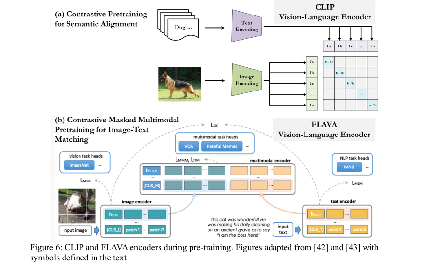
- CLIP (Contrastive Language–Image Pre-training) by OpenAI
- FLAVA (Foundational Language and Vision Alignment) by Meta AI
These models are pre-trained on massive datasets of image-text pairs, enabling them to perform zero-shot classification—that is, classifying new, unseen data without task-specific retraining.
The Challenge: Bridging Data, Information, and Expert Knowledge
The paper addresses a fundamental gap in materials engineering: the disconnect between raw data and expert knowledge.
As illustrated in the Data–Information–Knowledge–Wisdom (DIKW) hierarchy (Figure 1 in the paper), the journey from raw micrographs to qualified materials involves multiple steps:
- Data: Raw pixel intensities from optical metallography.
- Information: Extracted features via semantic segmentation (e.g., carbide clusters, porosity).
- Knowledge: Expert interpretation of these features using domain-specific criteria.
- Wisdom: Application-specific decisions (e.g., accept/reject based on industry standards).
While deep learning models excel at converting data to information, the information-to-knowledge transition remains largely manual. This is where customized VLRs come in.
The Solution: Customized and Hybrid VLRs
The study introduces a novel framework that enhances generic VLRs through customization and hybridization, specifically tailored for industrial qualification of additively manufactured metal matrix composites (MMCs).
Step 1: Data and Preprocessing
The researchers used Ni-WC MMCs fabricated via directed energy deposition (DED), a form of AM. Optical metallography images were processed and segmented using a deep learning tool called MicroSegQ+, which identified key phases:
- Red: Fusion line
- Blue: Heat-affected zone (HAZ)
- Green: Bead reinforcement area
- Pink: Carbide particles
- Dark Blue: Porosity
This segmentation transformed raw images into quantifiable microstructure information.
Step 2: Encoding Expert Knowledge
Six Expert Assessments (EAs) were defined to qualify the microstructures:
| ASSESSMENT | CRITERIA |
|---|---|
| Dilution (EA-1) | Area of matrix material mixing into substrate (≤5% acceptable) |
| HAZ (EA-2) | Depth of thermally altered substrate (≤1 mm typical) |
| Reinforcement (EA-3) | Presence of distinct bead structure |
| Porosity (EA-4) | Pore size, area fraction, distribution |
| Carbide Dissolution (EA-5) | ≥30% carbide area fraction |
| Carbide Distribution (EA-6) | Uniform spatial distribution |
Each assessment was encoded into positive and negative textual prompts, such as:
“An ideal microstructural image has uniformly distributed pink carbide particles in the green metal matrix…”
These color-aware textual descriptions were crucial for aligning language with visual features.
How Customized VLRs Work: The Net Similarity Scoring Approach
The core innovation lies in a customized similarity-based representation that computes a net similarity score for each microstructure.
1. Vision-Language Similarity (Using CLIP)
For a given image, the model computes cosine similarity with averaged positive and negative text embeddings:
\[ \bar{z}_T^{+} = \frac{1}{N^{+}} \sum_{i} z_{i}^{T+}, \quad \bar{z}_T^{-} = \frac{1}{N^{-}} \sum_{j} z_{j}^{T-} \] \[ \Delta_{\text{CLIP}} = \cos(z_I, \bar{z}_T^{+}) – \cos(z_I, \bar{z}_T^{-}) \]A positive Δ indicates alignment with acceptable criteria.
2. Vision-Vision Similarity (Using FLAVA)
Similarly, the model compares the query image to reference positive and negative image embeddings:
\[ \bar{z}_{I}^{+} = \frac{1}{M^{+}} \sum_{k} z_{k}^{I^{+}}, \quad \bar{z}_{I}^{-} = \frac{1}{M^{-}} \sum_{l} z_{l}^{I^{-}} \] \[ \Delta_{\text{FLAVA}} = \cos(z_q, \bar{z}_{I}^{+}) – \cos(z_q, \bar{z}_{I}^{-}) \]3. Hybridization via Z-Score Normalization
To combine both models, the deltas are z-score normalized to align their distributions:
\[ z_{\text{CLIP}} = \frac{\Delta_{\text{CLIP}} – \mu_{\text{CLIP}}}{\sigma_{\text{CLIP}}}, \qquad z_{\text{FLAVA}} = \frac{\Delta_{\text{FLAVA}} – \mu_{\text{FLAVA}}}{\sigma_{\text{FLAVA}}} \]The final hybrid similarity score is:
\[ \Delta_{\text{Hybrid}} = z_{\text{CLIP}} + z_{\text{FLAVA}} \]If ΔHybrid≥0 , the sample is classified as acceptable.
Key Findings: CLIP vs. FLAVA – Complementary Strengths
The study revealed distinct performance profiles:
| MODEL | STRENGTH | LIMITATION |
|---|---|---|
| CLIP | Strongtextual alignment; robust to phrasing variations | Lower visual sensitivity |
| FLAVA | Highvisual discrimination; better at image-to-image similarity | Sensitive to textual rewording |
For example:
- CLIP showed higher intra-class similarity among paraphrased technical descriptions.
- FLAVA produced more discriminative visual embeddings, suppressing spurious similarities.
The hybrid approach leveraged both strengths, significantly improving classification accuracy.
Performance Evaluation: Top-K Accuracy and Classification Results
The models were evaluated using top-K accuracy across individual and cumulative expert assessments.
Table: Top-5 Accuracy – Individual vs. Cumulative Assessments
| ASSESSMENT | FLAVA (TOP-5) | CLIP (TOP-5) | CLIP + COLOR (TOP-5) |
|---|---|---|---|
| Dilution (EA1) | 60% | 60% | 40% →60% |
| Porosity (EA3) | 40% | 20% | 20% →50% |
| Distribution (EA5) | 80% | 80% | 80% →80% |
Note: CLIP with color-aware prompts showed improved mid-rank retrieval.
Classification Outcomes
- Distribution: 4 false positives, 3 false negatives
- Dilution: 4 false positives (mostly negligible dilution)
- Reinforcement Area: 7 false positives (due to other defects not in reference set)
Z-score normalization played a critical role in correcting borderline cases. For instance:
- Sample 2: Negative raw CLIP delta (−0.0038) → Positive after normalization (0.1276) → Correct positive classification.
- Sample 3: Positive FLAVA delta (0.0772) but negative CLIP z-score (−0.7706) → Final negative classification.
Why Hybrid VLRs Outperform Single Models
The hybrid framework offers several advantages:
✅ Balanced Decision-Making: Combines textual robustness (CLIP) with visual sensitivity (FLAVA)
✅ No Retraining Needed: Operates in zero-shot mode, ideal for industrial agility
✅ Interpretable Results: Net similarity scores provide traceability
✅ Scalable Customization: New criteria can be added via textual prompts
As the authors state:
“Z-score normalization plays a critical role in shifting borderline decisions and aligning the influence of each modality in the final prediction.”
Industrial Application: A Multi-Modal Qualification Knowledge Base
The paper proposes a vision-language detection tree (Figure 32) for automated, high-throughput qualification:
- Input: New micrograph uploaded
- Segmentation: DL model extracts features
- Similarity Scoring: Hybrid VLR computes ΔHybrid
- Decision: Accept/Reject based on threshold
- Output: Classification + aligned textual rationale
Proposed UI Features (Figure 33):
- Interactive Fusion Strategy Selection (z-score sum, weighted average)
- Configurable Confidence Thresholding
- Dual-Model Backend (CLIP + FLAVA)
- Drag-and-Drop Image Upload
- Contextualized Expert Feedback Output
This system enables human-in-the-loop decision-making without requiring AI expertise.
SEO-Optimized Takeaways for Industry Professionals
🔍 Primary Keywords
- Vision-language representations
- Industrial qualification
- Additive manufacturing
- Microstructure informatics
- Expert knowledge integration
📌 Why This Matters for Your Business
- Reduce inspection time from hours to seconds
- Standardize quality control across facilities
- Preserve expert knowledge in a reusable format
- Enable rapid qualification of new materials and processes
🚀 Future-Ready Applications
- Integration with digital twins and in-situ monitoring
- Expansion to SEM, XCT, and EBSD data
- Prompt engineering for dynamic criteria updates
Conclusion: A New Era of AI-Augmented Materials Engineering
This study demonstrates that customized and hybrid vision-language representations can effectively bridge the gap between raw microstructural data and expert knowledge. By leveraging CLIP for stable textual alignment and FLAVA for sensitive visual discrimination, the framework enables zero-shot, interpretable, and scalable qualification of advanced materials.
The z-score normalized hybrid scoring method ensures robust decisions, even near classification boundaries. Moreover, the modular design allows seamless integration into existing industrial workflows.
As additive manufacturing continues to grow, such AI-augmented systems will become essential for high-throughput, reliable, and traceable material qualification.
Call to Action: Embrace the Future of Industrial AI
Are you ready to transform your materials qualification process?
👉 Download the full paper to explore the methodology in depth.
👉 Contact research teams at McGill University or NRC Canada for collaboration opportunities.
👉 Experiment with CLIP and FLAVA models using open-source implementations on Hugging Face or GitHub.
Don’t let manual inspection slow you down.
Leverage vision-language AI to build smarter, faster, and more reliable manufacturing pipelines.
Here is the complete Python script that implements the framework using the CLIP and FLAVA models.
# -*- coding: utf-8 -*-
"""
This script implements the end-to-end model proposed in the paper:
"Linking heterogeneous microstructure informatics with expert characterization
knowledge through customized and hybrid vision-language representations for
industrial qualification" by Mutahar Safdar et al.

The code performs zero-shot classification of microstructural images based on
customized and hybrid similarity scores from pre-trained CLIP and FLAVA models.
"""

# Install necessary libraries if they are not already installed.
# !pip install transformers torch Pillow numpy scikit-learn

import torch
from transformers import CLIPProcessor, CLIPModel, FlavaProcessor, FlavaModel
from PIL import Image
import numpy as np
from sklearn.metrics import confusion_matrix, classification_report
import os
import requests
from io import BytesIO

# --- 1. Model Loading ---
def load_models():
    """Loads the pre-trained CLIP and FLAVA models and processors."""
    print("Loading pre-trained models (CLIP and FLAVA)...")
    # Load CLIP model and processor from Hugging Face
    clip_model = CLIPModel.from_pretrained("openai/clip-vit-base-patch32")
    clip_processor = CLIPProcessor.from_pretrained("openai/clip-vit-base-patch32")

    # Load FLAVA model and processor from Hugging Face
    flava_model = FlavaModel.from_pretrained("facebook/flava-full")
    flava_processor = FlavaProcessor.from_pretrained("facebook/flava-full")
    print("Models loaded successfully.")
    return clip_model, clip_processor, flava_model, flava_processor

# --- 2. Feature Extraction ---
def get_image_embedding(image_path, model, processor):
    """Extracts feature embedding from a single image."""
    try:
        # Check if the image_path is a URL or a local file
        if image_path.startswith('http'):
            response = requests.get(image_path)
            image = Image.open(BytesIO(response.content)).convert("RGB")
        else:
            image = Image.open(image_path).convert("RGB")
    except (IOError, FileNotFoundError):
        print(f"Error: Image file not found at {image_path}")
        return None

    # Preprocess the image and get the pixel values
    inputs = processor(images=image, return_tensors="pt")
    with torch.no_grad():
        # Get the image features (embedding)
        if "clip" in model.config.model_type:
            embedding = model.get_image_features(pixel_values=inputs['pixel_values'])
        else: # FLAVA
            embedding = model.get_image_features(pixel_values=inputs['pixel_values'])
    # L2 normalize the embedding as per the paper's methodology
    embedding = embedding / embedding.norm(p=2, dim=-1, keepdim=True)
    return embedding

def get_text_embedding(text, model, processor):
    """Extracts feature embedding from a text prompt."""
    inputs = processor(text=text, return_tensors="pt", padding=True, truncation=True)
    with torch.no_grad():
        # Get the text features (embedding)
        if "clip" in model.config.model_type:
            embedding = model.get_text_features(**inputs)
        else: # FLAVA - Note: FLAVA text embeddings are not directly comparable to image embeddings
            embedding = model.get_text_features(**inputs)
    # L2 normalize the embedding
    embedding = embedding / embedding.norm(p=2, dim=-1, keepdim=True)
    return embedding

def get_mean_embedding(paths, model, processor, input_type='image'):
    """Computes the mean embedding for a list of images or texts."""
    embeddings = []
    for path in paths:
        if input_type == 'image':
            emb = get_image_embedding(path, model, processor)
        else:
            emb = get_text_embedding(path, model, processor)
        if emb is not None:
            embeddings.append(emb)
    if not embeddings:
        return None
    # Stack embeddings and calculate the mean
    mean_emb = torch.mean(torch.stack(embeddings), dim=0)
    # Re-normalize the mean embedding
    mean_emb = mean_emb / mean_emb.norm(p=2, dim=-1, keepdim=True)
    return mean_emb

# --- 3. Similarity and Scoring ---
def cosine_similarity(emb1, emb2):
    """Computes cosine similarity between two embeddings."""
    # Ensure embeddings are on the same device and correctly shaped
    emb1 = emb1.cpu().numpy().flatten()
    emb2 = emb2.cpu().numpy().flatten()
    return np.dot(emb1, emb2) / (np.linalg.norm(emb1) * np.linalg.norm(emb2))

def calculate_delta_scores(image_paths, clip_model, clip_processor, flava_model, flava_processor, pos_img_refs, neg_img_refs, pos_text_refs, neg_text_refs):
    """Calculates the raw delta scores for CLIP and FLAVA for all images."""
    print("\nCalculating delta scores for the dataset...")
    # Get mean reference embeddings
    mean_pos_img_flava = get_mean_embedding(pos_img_refs, flava_model, flava_processor, 'image')
    mean_neg_img_flava = get_mean_embedding(neg_img_refs, flava_model, flava_processor, 'image')
    mean_pos_text_clip = get_mean_embedding(pos_text_refs, clip_model, clip_processor, 'text')
    mean_neg_text_clip = get_mean_embedding(neg_text_refs, clip_model, clip_processor, 'text')

    delta_flava_scores = []
    delta_clip_scores = []

    for img_path in image_paths:
        # Get embeddings for the current input image
        img_emb_flava = get_image_embedding(img_path, flava_model, flava_processor)
        img_emb_clip = get_image_embedding(img_path, clip_model, clip_processor)

        if img_emb_flava is None or img_emb_clip is None:
            continue

        # Calculate FLAVA (vision-vision) similarity delta (Equation 8)
        sim_pos_flava = cosine_similarity(img_emb_flava, mean_pos_img_flava)
        sim_neg_flava = cosine_similarity(img_emb_flava, mean_neg_img_flava)
        delta_flava = sim_pos_flava - sim_neg_flava
        delta_flava_scores.append(delta_flava)

        # Calculate CLIP (vision-language) similarity delta (Equation 6)
        sim_pos_clip = cosine_similarity(img_emb_clip, mean_pos_text_clip)
        sim_neg_clip = cosine_similarity(img_emb_clip, mean_neg_text_clip)
        delta_clip = sim_pos_clip - sim_neg_clip
        delta_clip_scores.append(delta_clip)

    return np.array(delta_flava_scores), np.array(delta_clip_scores)

def z_score_normalize(scores):
    """Applies z-score normalization to a list of scores."""
    mean = np.mean(scores)
    std = np.std(scores)
    if std == 0:
        return np.zeros_like(scores)
    return (scores - mean) / std

# --- 4. Main Classification Logic ---
def classify_microstructures(image_paths, delta_flava_scores, delta_clip_scores):
    """Classifies images using the hybrid scoring method."""
    print("\nNormalizing scores and performing hybrid classification...")
    # Normalize the delta scores using z-score (Equations 9 & 10)
    z_flava = z_score_normalize(delta_flava_scores)
    z_clip = z_score_normalize(delta_clip_scores)

    # Calculate the final hybrid score (Equation 11)
    hybrid_scores = z_clip + z_flava

    # Classify based on the hybrid score
    # "Positive" if score >= 0, "Negative" if score < 0
    predictions = ["Positive" if score >= 0 else "Negative" for score in hybrid_scores]

    print("\n--- Classification Results ---")
    for i, img_path in enumerate(image_paths):
        print(f"Image: {os.path.basename(img_path):<15} | Δ_FLAVA: {delta_flava_scores[i]:.4f} (z={z_flava[i]:.4f}) | Δ_CLIP: {delta_clip_scores[i]:.4f} (z={z_clip[i]:.4f}) | Hybrid Score: {hybrid_scores[i]:.4f} | Prediction: {predictions[i]}")

    return predictions

# --- 5. Main Execution ---
if __name__ == "__main__":
    # --- Mock Dataset and Ground Truth ---
    # In a real scenario, this would be your dataset of image paths.
    # For demonstration, we'll use placeholder URLs.
    # Replace these with paths to your actual image files.
    # The paper uses 40 samples, but we'll use a smaller set for this example.

    # Let's create a dummy directory and some images for a local test
    if not os.path.exists("mock_images"):
        os.makedirs("mock_images")

    base_url = "https://placehold.co/600x400"
    image_files = {
        "sample1_good_dist.png": f"{base_url}/5cb85c/ffffff?text=Good+Dist", # Greenish
        "sample2_good_dist.png": f"{base_url}/6fbf6f/ffffff?text=Good+Dist", # Light Green
        "sample3_bad_dist.png": f"{base_url}/d9534f/ffffff?text=Bad+Dist", # Reddish
        "sample4_bad_dist.png": f"{base_url}/c9302c/ffffff?text=Bad+Dist", # Dark Red
        "sample5_good_dilution.png": f"{base_url}/5bc0de/ffffff?text=Good+Dilution", # Light Blue
        "sample6_bad_dilution.png": f"{base_url}/f0ad4e/ffffff?text=Bad+Dilution", # Orange
        "sample7_good_reinforce.png": f"{base_url}/292b2c/ffffff?text=Good+Reinforce", # Dark Grey
        "sample8_bad_reinforce.png": f"{base_url}/f7f7f7/000000?text=Bad+Reinforce" # Light Grey
    }

    for name, url in image_files.items():
        path = os.path.join("mock_images", name)
        if not os.path.exists(path):
            response = requests.get(url)
            with open(path, 'wb') as f:
                f.write(response.content)

    all_image_paths = [os.path.join("mock_images", f) for f in image_files.keys()]

    # Ground truth labels for each assessment (1 for Positive, 0 for Negative)
    # This is a mock ground truth for evaluation purposes.
    ground_truth = {
        "Distribution": [1, 1, 0, 0, 1, 0, 1, 0],
        "Dilution":     [1, 1, 1, 1, 1, 0, 1, 0],
        "Reinforcement":[1, 1, 1, 1, 1, 1, 1, 0]
    }

    # --- Reference Sets for Expert Assessments (based on the paper) ---
    # These should be paths to images and text prompts that define "good" vs "bad"
    expert_assessments = {
        "Distribution": {
            "pos_imgs": [os.path.join("mock_images", "sample1_good_dist.png")],
            "neg_imgs": [os.path.join("mock_images", "sample3_bad_dist.png")],
            "pos_texts": ["An ideal microstructural image has uniformly distributed pink carbide particles in the green metal matrix."],
            "neg_texts": ["A non-ideal microstructural image has uneven or clustered pink carbide particles in the green metal matrix."]
        },
        "Dilution": {
            "pos_imgs": [os.path.join("mock_images", "sample5_good_dilution.png")],
            "neg_imgs": [os.path.join("mock_images", "sample6_bad_dilution.png")],
            "pos_texts": ["An ideal microstructural image has the bead reinforcement area fully contained above the red fusion line, highlighting no dilution."],
            "neg_texts": ["A non-ideal microstructural image shows the bead reinforcement area intruding below the red fusion line, indicating dilution."]
        },
        "Reinforcement": {
            "pos_imgs": [os.path.join("mock_images", "sample7_good_reinforce.png")],
            "neg_imgs": [os.path.join("mock_images", "sample8_bad_reinforce.png")],
            "pos_texts": ["A green bead reinforcement area with pink carbide particles is present above the blue substrate."],
            "neg_texts": ["A non-ideal microstructural image shows an incomplete or poorly defined green bead reinforcement area."]
        }
    }

    # Load models
    clip_model, clip_processor, flava_model, flava_processor = load_models()

    # --- Run classification for each expert assessment ---
    for assessment, refs in expert_assessments.items():
        print(f"\n========================================================")
        print(f"PERFORMING ASSESSMENT FOR: {assessment.upper()}")
        print(f"========================================================")

        # 1. Calculate Delta Scores for all images
        delta_flava, delta_clip = calculate_delta_scores(
            all_image_paths,
            clip_model, clip_processor,
            flava_model, flava_processor,
            refs["pos_imgs"], refs["neg_imgs"],
            refs["pos_texts"], refs["neg_texts"]
        )

        # 2. Classify based on the scores
        predictions = classify_microstructures(all_image_paths, delta_flava, delta_clip)

        # 3. Evaluate the results
        true_labels_int = ground_truth[assessment]
        pred_labels_int = [1 if p == "Positive" else 0 for p in predictions]
        true_labels_str = ["Positive" if l == 1 else "Negative" for l in true_labels_int]

        print(f"\n--- Evaluation for {assessment} ---")
        try:
            print("Confusion Matrix:")
            print(confusion_matrix(true_labels_int, pred_labels_int))
            print("\nClassification Report:")
            print(classification_report(true_labels_str, predictions, zero_division=0))
        except Exception as e:
            print(f"Could not generate evaluation report. Error: {e}")
Related posts, You May like to read
- 7 Shocking Truths About Knowledge Distillation: The Good, The Bad, and The Breakthrough (SAKD)
- 7 Revolutionary Breakthroughs in Medical Image Translation (And 1 Fatal Flaw That Could Derail Your AI Model)
- DeepSPV: Revolutionizing 3D Spleen Volume Estimation from 2D Ultrasound with AI
- ACAM-KD: Adaptive and Cooperative Attention Masking for Knowledge Distillation
- GeoSAM2 3D Part Segmentation — Prompt-Controllable, Geometry-Aware Masks for Precision 3D Editing
- Probabilistic Smooth Attention for Deep Multiple Instance Learning in Medical Imaging
- A Knowledge Distillation-Based Approach to Enhance Transparency of Classifier Models
- Towards Trustworthy Breast Tumor Segmentation in Ultrasound Using AI Uncertainty