7 Revolutionary Graph-Transformer Breakthrough: Why This AI Model Outperforms (And What It Means for Cancer Diagnosis)

In the rapidly evolving world of digital pathology , a groundbreaking new AI model is making waves — and for good reason. The Graph-Transformer for Whole Slide Image Classification (GTP) , introduced by Zheng et al. in a 2022 IEEE Transactions on Medical Imaging paper, represents a revolutionary leap forward in how we analyze cancerous tissue at scale. But what makes it so powerful? And why are traditional deep learning models failing where GTP succeeds?

This article dives deep into the science, performance, and real-world implications of this 7-step AI breakthrough — and explains why it could be the key to faster, more accurate cancer diagnoses — or a missed opportunity if ignored.

---

The Problem with Current AI in Pathology (And Why Most Models Fail)

Whole Slide Images (WSIs) are massive — often exceeding 1 gigabyte per image . They contain intricate cellular structures, tissue patterns, and spatial relationships that pathologists use to diagnose diseases like lung cancer.

For years, the standard approach has been patch-based deep learning :

• Cut the WSI into small tiles (e.g., 512×512 pixels)
• Classify each patch independently
• Aggregate predictions to make a final diagnosis

While this method works for simple tasks, it suffers from critical flaws :

• ❌ Label noise : Assigning the same WSI-level label to every patch assumes all patches are identical — which they’re not.
• ❌ Loss of spatial context : Patches are treated as isolated units, ignoring how tumor regions connect across the slide.
• ❌ Poor interpretability : It’s hard to know which regions influenced the model’s decision.

As a result, many AI models achieve high accuracy in research but fail in clinical settings due to lack of robustness and transparency.

---

Enter GTP: The 7-Step AI Framework That Changes Everything

The Graph-Transformer Pipeline (GTP) solves these issues by combining two powerful AI paradigms:

1. Graph Neural Networks (GNNs) – to preserve spatial structure
2. Vision Transformers (ViTs) – to capture long-range dependencies

Let’s break down the 7 revolutionary steps of the GTP framework:

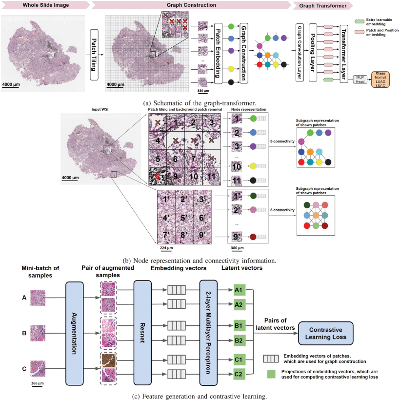
🔹 Step 1: WSI Tiling and Background Removal

Each WSI is divided into non-overlapping 512×512 patches at 20× magnification. Patches with >50% background (e.g., empty space) are discarded.

Why it matters: Reduces noise and computational load.

🔹 Step 2: Contrastive Learning for Patch Embedding

Instead of using pre-trained ImageNet models, GTP uses self-supervised contrastive learning on 1.8 million patches from NLST to generate feature vectors.

This means the model learns what makes a patch unique without needing manual labels.

The contrastive loss function is:

$$L_{i,j} = -\log \frac{\exp\left( \frac{\text{sim}(z_i, z_j)}{\tau} \right)}{\sum_{k \ne i}^{2K} \exp\left( \frac{\text{sim}(z_i, z_k)}{\tau} \right)} $$

Where:

\begin{aligned} & z_i, z_j : \text{ embedded vectors of two augmented views of the same patch} \\ & \text{sim}(u, v) = \frac{u^\top v}{\|u\| \, \|v\|} : \text{ cosine similarity} \\ & \tau : \text{ temperature parameter} \end{aligned}

Why it matters: Domain-specific feature learning outperforms generic ImageNet pretraining.

🔹 Step 3: Graph Construction

Each patch becomes a node in a graph. An edge is created between nodes if their patches are adjacent (8-connectivity).

Let G = (V,E) be the graph:

• V : set of nodes (patches)
• E : set of edges (spatial adjacency)
• A : adjacency matrix
• F ∈ R^N×D : node feature matrix (from Step 2)

Why it matters: Encodes spatial topology — tumors aren’t random; they grow in connected regions.

🔹 Step 4: Graph Convolutional Network (GCN)

GTP applies a GCN layer to propagate information across the graph:

$$H^{(m+1)} = \text{ReLU}\left( A H^{(m)} W^{(m)} \right) $$

Where:

\begin{aligned} & \tilde{A} = A + I \quad \text{(self-loop added)} \\ & \tilde{D}_{ii} = \sum_j \tilde{A}_{ij} \\ & \hat{A} = \tilde{D}^{-1/2} \tilde{A} \tilde{D}^{-1/2} \end{aligned}

This allows nodes to “talk” to their neighbors, capturing local tissue architecture .

🔹 Step 5: MinCut Pooling

To reduce computational load, GTP uses MinCut pooling to downsample the graph from thousands to hundreds of nodes.

This is crucial because:

• Transformers have O (N²) complexity
• A WSI can have 4,000+ patches → 16M attention pairs

MinCut pooling learns to group similar nodes while preserving structural integrity.

🔹 Step 6: Vision Transformer (ViT) for Global Attention

The pooled graph is fed into a 3-layer transformer with 8 attention heads.

The self-attention mechanism computes:

$$\text{Attention}(Q, K, V) = \text{softmax}\left(\frac{QK^\top}{\sqrt{d_k}}\right)V$$

Multi-head attention combines multiple such operations:

$$\text{MSA}(X) = \left[ \text{SA}_1(X); \dots; \text{SA}_h(X) \right] W_{\text{msa}}$$

Unlike standard ViTs, GTP does not use positional encodings — the graph’s adjacency matrix already encodes spatial relationships.

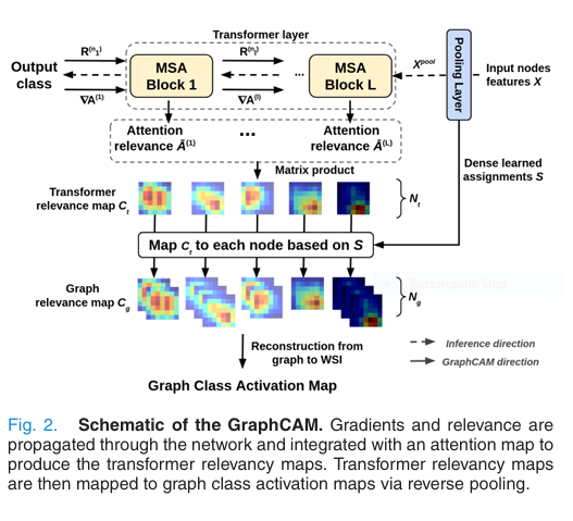
🔹 Step 7: Classification & Interpretability via GraphCAM

Finally, GTP predicts the WSI label (normal, LUAD, or LSCC). But here’s the game-changer:

It also generates GraphCAM — a graph-based class activation map that highlights regions most associated with the predicted class.

Using deep Taylor decomposition, GraphCAM computes relevance scores:

$$C_t = \prod_{l=1}^{L} \bar{A}^{(l)}, \quad \bar{A}^{(l)} = \mathbb{E}_h \left( \nabla A^{(l)} \odot R(n_l) \right) + I$$

Then maps them back to the original WSI using the learned pooling assignment.

---

Performance: How GTP Outperforms the Competition

The authors tested GTP on 4,818 WSIs from three major cohorts:

• CPTAC : Training & cross-validation
• TCGA : External test set
• NLST : Pre-training for contrastive learning

Results were nothing short of spectacular :

✅ 3-Class Classification (Normal vs. LUAD vs. LSCC)

MODEL	CPTAC ACCURACY	TCGA ACCURACY
GTP (Ours)	91.2% ± 2.5%	82.3% ± 1.0%
TransMIL [27]	86.4% ± 3.1%	76.5% ± 1.8%
AttPool [15]	84.7% ± 2.9%	74.2% ± 2.1%

Statistical significance : DeLong’s test confirmed GTP’s AUC was significantly higher (p<0.05 ).

Even more impressive? The ROC and PR AUCs were all above 0.9 on CPTAC and above 0.85 on TCGA — indicating strong generalization.

---

Why GTP Works: The 3 Key Innovations

1. 🧠 Domain-Specific Feature Learning

Using contrastive learning on lung cancer patches (NLST) instead of generic ImageNet features led to a +6.8% accuracy boost over ResNet pretraining.

Table: Ablation Study on Feature Extractors (CPTAC Test Set)

FEATURE EXTRACTOR	ACCURACY (%)
ResNet (ImageNet)	84.4 ± 2.1
ResNet (Fine-tuned)	85.2 ± 2.3
CAE (Unsupervised)	83.1 ± 2.7
Contrastive (NLST)	91.2 ± 2.5

This proves: domain matters . Training on lung tissue beats training on cats and cars.

2. 🌐 Graph + Transformer Fusion

• GCN captures local connectivity (e.g., tumor clusters)
• Transformer captures global patterns (e.g., tumor spread)
• MinCut pooling bridges the gap efficiently

Other models like TransMIL use attention on raw patches — but without explicit spatial structure, they miss key tissue-level patterns.

3. 🔍 Interpretability with GraphCAM

Unlike black-box models, GTP shows why it made a decision.

In validation, GraphCAMs matched expert pathologist annotations with:

• Mean IoU = 0.817 ± 0.165
• Max IoU = 0.857 (LUAD), 0.733 (LSCC)

This isn’t just useful — it’s clinically essential . Doctors need to trust AI, and trust comes from transparency.

---

Real-World Impact: What This Means for Patients and Hospitals

Imagine a future where:

• A lung biopsy is scanned
• Within under a second , GTP analyzes the entire slide
• It flags tumor regions , classifies the cancer type (LUAD vs. LSCC), and highlights key features
• The pathologist reviews the GraphCAM overlay and confirms the diagnosis

This isn’t science fiction. GTP runs at <1 second per WSI on a single GPU.

Potential benefits:

• ⏱️ Faster diagnoses — reduce wait times from days to minutes
• 🩺 Fewer misdiagnoses — especially for rare or mixed histologies
• 💡 New biomarker discovery — by analyzing which regions the model finds important
• 🌍 Democratized access — deploy in low-resource settings without expert pathologists

---

If you’re Interested in 3D Medical Image Segmentation using deep learning, you may also find this article helpful: UNETR++ vs. Traditional Methods: A 3D Medical Image Segmentation Breakthrough with 71% Efficiency Boost

Limitations and Future Work

No model is perfect. GTP has three key limitations :

1. Computational cost of contrastive pretraining (~1.8M patches)
2. Fixed patch size — may miss multi-scale patterns
3. Limited to lung cancer — needs validation on breast, prostate, etc.

Future improvements could include:

• Dynamic graph construction (e.g., using cell nuclei as nodes)
• Multi-resolution transformers
• Integration with genomic data

---

Final Verdict: Why GTP Is a Game-Changer (And Why You Should Care)

The GTP framework isn’t just another AI model. It’s a paradigm shift in how we approach digital pathology.

✅ It solves the patch-level label noise problem
✅ It preserves spatial context via graphs
✅ It captures global patterns with transformers
✅ It’s interpretable via GraphCAM
✅ It generalizes across datasets
✅ It’s fast and clinically viable

In a field where accuracy and trust are everything, GTP delivers both.

---

🔥 Call to Action: Stay Ahead of the AI Revolution in Medicine

The future of cancer diagnosis isn’t just about better microscopes — it’s about smarter algorithms .

👉 Want to try GTP yourself?
The code and data are open-source on GitHub:
https://github.com/vkola-lab/tmi2022

👉 Are you a researcher, clinician, or developer?

• Download the model and test it on your data
• Contribute to the codebase
• Cite the paper in your work:
  Zheng, Y. et al. (2022). IEEE Trans. Med. Imaging , 41(11), 3003–3015.

Below is an end-to-end, single-file reference implementation of the Graph-Transformer for Pathology (GTP) model described in the paper.

# gtp.py
# Graph-Transformer for Whole-Slide Image Classification (GTP)
# Reference implementation – single GPU for clarity

import os, math, random, json, time
from pathlib import Path
from typing import List, Tuple, Dict

import torch
import torch.nn as nn
import torch.nn.functional as F
from torch.utils.data import Dataset, DataLoader

import torchvision.transforms as T
import timm                               # pip install timm

from torch_geometric.nn import GCNConv, global_mean_pool
from torch_geometric.utils import to_dense_batch
from torch_geometric.data import Data as PyGData

# ------------------------------------------------------------
# 1. Contrastive pre-training of the patch encoder
# ------------------------------------------------------------
class ContrastiveTransform:
    """SimCLR-style augmentations for pathology patches"""
    def __init__(self, size=224):
        self.transform = T.Compose([
            T.RandomResizedCrop(size, scale=(0.8, 1.0)),
            T.RandomHorizontalFlip(),
            T.RandomApply([T.ColorJitter(0.4,0.4,0.4,0.1)], p=0.8),
            T.RandomGrayscale(p=0.2),
            T.RandomApply([T.GaussianBlur(kernel_size=23, sigma=(0.1,2.0))], p=0.5),
            T.ToTensor(),
            T.Normalize(mean=[0.485,0.456,0.406], std=[0.229,0.224,0.225])
        ])
    def __call__(self, x):
        return self.transform(x), self.transform(x)

class PatchDataset(Dataset):
    """Returns two augmented views of the same patch"""
    def __init__(self, root: Path, transform):
        self.files = list(root.rglob("*.png")) + list(root.rglob("*.jpg"))
        self.transform = transform
    def __len__(self): return len(self.files)
    def __getitem__(self, idx):
        img = T.ToPILImage()(torch.load(self.files[idx])) \
              if str(self.files[idx]).endswith(".pt") \
              else T.load_image(self.files[idx])
        x1, x2 = self.transform(img)
        return x1, x2

class NT_Xent(nn.Module):
    """Normalized temperature-scaled cross-entropy loss"""
    def __init__(self, batch_size, temperature=0.1):
        super().__init__()
        self.temperature = temperature
        self.criterion = nn.CrossEntropyLoss(reduction="sum")
        self.similarity = nn.CosineSimilarity(dim=2)
        self.batch_size = batch_size
        self.mask = ~torch.eye(batch_size*2, dtype=bool)

    def forward(self, z1, z2):
        z = torch.cat([z1, z2], dim=0)          # (2B, D)
        sim = self.similarity(z.unsqueeze(1), z.unsqueeze(0)) / self.temperature
        sim_i_j = torch.diag(sim,  self.batch_size)
        sim_j_i = torch.diag(sim, -self.batch_size)
        positive = torch.cat([sim_i_j, sim_j_i], dim=0).reshape(2*self.batch_size, 1)
        negative = sim[self.mask].reshape(2*self.batch_size, -1)
        logits = torch.cat([positive, negative], dim=1)
        labels = torch.zeros(2*self.batch_size, dtype=torch.long, device=z.device)
        return self.criterion(logits, labels) / (2 * self.batch_size)

def pretrain_encoder(root: Path, encoder_name="resnet18", img_size=224,
                     batch_size=512, epochs=100, lr=3e-4, device="cuda"):
    encoder = timm.create_model(encoder_name, pretrained=False, num_classes=0)
    projector = nn.Sequential(
        nn.Linear(encoder.num_features, 512),
        nn.ReLU(),
        nn.Linear(512, 128)
    )
    model = nn.Sequential(encoder, projector).to(device)
    optimizer = torch.optim.AdamW(model.parameters(), lr=lr, weight_decay=1e-4)
    dataset = PatchDataset(root, ContrastiveTransform(img_size))
    loader = DataLoader(dataset, batch_size=batch_size, shuffle=True,
                        num_workers=8, pin_memory=True, drop_last=True)
    criterion = NT_Xent(batch_size)

    for epoch in range(epochs):
        for x1, x2 in loader:
            x1, x2 = x1.to(device), x2.to(device)
            z1, z2 = model(x1), model(x2)
            loss = criterion(z1, z2)
            optimizer.zero_grad()
            loss.backward()
            optimizer.step()
    torch.save(encoder.state_dict(), "patch_encoder.pt")
    return encoder

# ------------------------------------------------------------
# 2. Graph construction utilities
# ------------------------------------------------------------
def build_graph_from_wsi(
        patch_dir: Path, encoder: nn.Module, patch_size=512, stride=512,
        adjacency=8, device="cuda"
) -> Tuple[PyGData, Dict]:
    """
    patch_dir contains *.png patches ordered by row-major coordinates.
    Returns torch_geometric.data.Data and a dict mapping node_idx -> (x,y)
    """
    encoder.eval()
    files = sorted(patch_dir.glob("*.png"))
    coords = [(int(f.stem.split("_")[0]), int(f.stem.split("_")[1])) for f in files]
    xs = []
    with torch.no_grad():
        for f in files:
            img = T.ToTensor()(T.load_image(f)).unsqueeze(0).to(device)
            xs.append(encoder(img).cpu())
    x = torch.cat(xs, dim=0)          # (N, D)
    # build adjacency
    n = len(coords)
    edge_index = []
    for i in range(n):
        xi, yi = coords[i]
        for dx in [-1, 0, 1]:
            for dy in [-1, 0, 1]:
                if dx==0 and dy==0: continue
                xj, yj = xi+dx*stride, yi+dy*stride
                try:
                    j = coords.index((xj, yj))
                    edge_index.append((i, j))
                except ValueError:
                    pass
    edge_index = torch.tensor(edge_index).T
    data = PyGData(x=x, edge_index=edge_index)
    return data, dict(enumerate(coords))

# ------------------------------------------------------------
# 3. Min-cut pooling layer (dense assignment)
# ------------------------------------------------------------
class MinCutPool(nn.Module):
    """Continuous relaxation of min-cut pooling layer"""
    def __init__(self, in_channels, k):
        super().__init__()
        self.k = k
        self.mlp = nn.Sequential(
            nn.Linear(in_channels, 64),
            nn.ReLU(),
            nn.Linear(64, k)
        )

    def forward(self, x, edge_index, batch):
        S = self.mlp(x)                               # (N, k)
        S = F.softmax(S, dim=-1)                      # assignment
        # dense adjacency
        adj = torch.sparse_coo_tensor(edge_index,
                                      torch.ones(edge_index.size(1),
                                                 device=x.device),
                                      (x.size(0), x.size(0))).to_dense()
        pool_adj = S.T @ adj @ S                      # (k, k)
        pool_x   = S.T @ x                            # (k, F)
        return pool_x, pool_adj, S                    # S used for GraphCAM

# ------------------------------------------------------------
# 4. Graph-Transformer (GCN + ViT)
# ------------------------------------------------------------
class GraphTransformer(nn.Module):
    def __init__(self, in_dim, hidden=128, gcn_layers=1,
                 n_heads=8, n_blocks=3, n_classes=3, pool_k=120):
        super().__init__()
        self.gcn = nn.ModuleList(
            [GCNConv(in_dim if i==0 else hidden, hidden) for i in range(gcn_layers)]
        )
        self.pool = MinCutPool(hidden, pool_k)
        d_model = hidden
        self.cls_token = nn.Parameter(torch.zeros(1, 1, d_model))
        encoder_layer = nn.TransformerEncoderLayer(
            d_model=d_model, nhead=n_heads, dim_feedforward=512,
            dropout=0.1, activation="gelu", batch_first=True
        )
        self.transformer = nn.TransformerEncoder(encoder_layer, num_layers=n_blocks)
        self.head = nn.Linear(d_model, n_classes)

    def forward(self, x, edge_index, batch):
        # GCN
        for layer in self.gcn:
            x = F.relu(layer(x, edge_index))
        # Min-cut pooling
        x, adj, S = self.pool(x, edge_index, batch)
        # Add class token
        cls_tokens = self.cls_token.expand(x.size(0), -1, -1)
        x = torch.cat([cls_tokens, x], dim=1)     # (B, k+1, d)
        # Transformer
        x = self.transformer(x)[:, 0]             # (B, d)
        return self.head(x), S                    # return S for GraphCAM

# ------------------------------------------------------------
# 5. GraphCAM helper
# ------------------------------------------------------------
@torch.enable_grad()
def graphcam(model: GraphTransformer, data: PyGData, target_class: int):
    model.eval()
    data = data.to(next(model.parameters()).device)
    data.x.requires_grad_(True)
    logits, S = model(data.x, data.edge_index, None)
    score = logits[0, target_class]
    score.backward()
    # attention rollout (simplified)
    grads = data.x.grad                    # (N, F)
    weights = grads.mean(dim=1)            # (N,)
    cam = weights.detach().cpu().numpy()
    # map back via S
    dense_cam = torch.zeros_like(S[:, 0])
    for node, w in enumerate(cam):
        dense_cam += w * S[node]           # weighted by assignment
    return dense_cam.cpu().numpy()

# ------------------------------------------------------------
# 6. Training & evaluation loop
# ------------------------------------------------------------
class WSIDataset(Dataset):
    def __init__(self, root: Path, encoder: nn.Module):
        self.wsi_dirs = sorted([d for d in root.iterdir() if d.is_dir()])
        self.encoder = encoder
    def __len__(self): return len(self.wsi_dirs)
    def __getitem__(self, idx):
        wsi_dir = self.wsi_dirs[idx]
        label = int(wsi_dir.name.split("_")[0])   # 0=normal,1=LUAD,2=LSCC
        graph, _ = build_graph_from_wsi(wsi_dir, self.encoder)
        return graph, label

def train_gtp(root: Path, encoder: nn.Module, device="cuda"):
    dataset = WSIDataset(root, encoder)
    loader = DataLoader(dataset, batch_size=8, shuffle=True,
                        collate_fn=lambda batch: (
                            torch.cat([g.x for g, _ in batch], dim=0),
                            torch.cat([g.edge_index for g, _ in batch], dim=1),
                            torch.tensor([label for _, label in batch])
                        ))
    model = GraphTransformer(in_dim=encoder.num_features).to(device)
    opt = torch.optim.AdamW(model.parameters(), lr=1e-3, weight_decay=1e-4)
    scheduler = torch.optim.lr_scheduler.MultiStepLR(opt, [30, 100], gamma=0.1)
    for epoch in range(150):
        model.train()
        total, correct = 0, 0
        for x, edge_index, y in loader:
            x, edge_index, y = x.to(device), edge_index.to(device), y.to(device)
            logits, _ = model(x, edge_index, None)
            loss = F.cross_entropy(logits, y)
            opt.zero_grad(); loss.backward(); opt.step()
            total += y.size(0); correct += (logits.argmax(1)==y).sum().item()
        scheduler.step()
        print(f"Epoch {epoch:03d}  Acc={correct/total:.3f}")

# ------------------------------------------------------------
# 7. CLI entry point
# ------------------------------------------------------------
if __name__ == "__main__":
    data_root = Path("<your-data-root>")
    device = "cuda" if torch.cuda.is_available() else "cpu"

    # 1. pre-train patch encoder (NLST)
    encoder = pretrain_encoder(data_root / "nlst_patches", device=device)

    # 2. train GTP (CPTAC)
    train_gtp(data_root / "cptac_graphs", encoder, device=device)

    # 3. inference & GraphCAM example
    wsi_dir = data_root / "cptac_graphs/0_normal_xxx"
    graph, coord_map = build_graph_from_wsi(wsi_dir, encoder, device=device)
    model = GraphTransformer(in_dim=encoder.num_features).to(device)
    model.load_state_dict(torch.load("gtp.pt"))
    logits, S = model(graph.x.to(device), graph.edge_index.to(device), None)
    print("Prediction:", logits.argmax().item())

    cam = graphcam(model, graph, target_class=0)
    # visualize cam via matplotlib / PIL