Introduction: The Evolution of Medical Image Segmentation
Medical image segmentation plays a pivotal role in diagnostics, treatment planning, and clinical research. As technology advances, the demand for accurate, efficient, and scalable segmentation methods has never been higher. However, the field faces a significant challenge: limited labeled data . Annotating medical images is time-consuming, expensive, and requires expert knowledge.
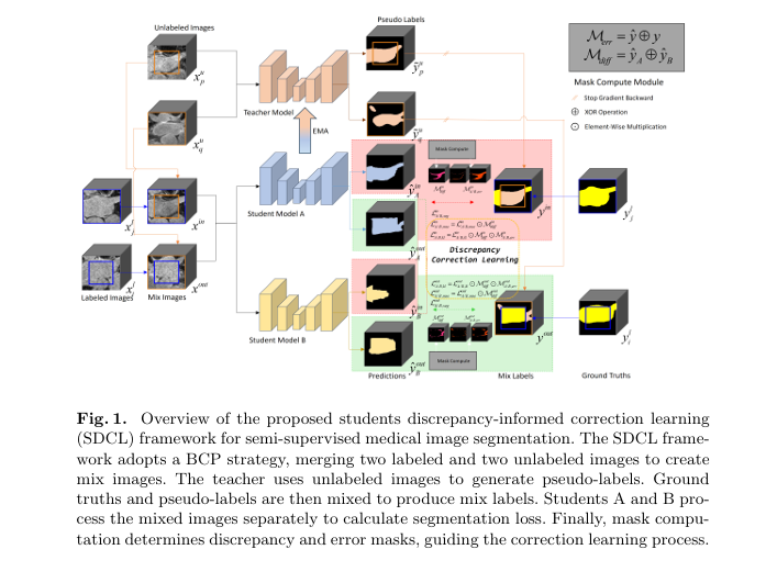
This is where semi-supervised learning (SSL) comes into play. By leveraging both labeled and unlabeled data , SSL methods aim to bridge the gap between limited supervision and high performance. One of the most promising innovations in this space is SDCL (Students Discrepancy-Informed Correction Learning) — a novel framework that redefines how we approach medical image segmentation by addressing the confirmation and cognitive biases that plague traditional teacher-student models.
In this article, we’ll explore how SDCL works, its advantages over existing methods, and the mathematical foundation that powers its superior performance. Whether you’re a researcher, developer, or healthcare professional, this guide will provide valuable insights into the future of medical imaging.
What is SDCL? A Game-Changer in Semi-Supervised Medical Image Segmentation
Understanding the SDCL Framework
SDCL introduces a three-model architecture consisting of:
- Two structurally different students (Student A and Student B)
- One non-trainable teacher (based on Exponential Moving Average or EMA)
Unlike traditional Mean Teacher (MT) frameworks that rely on a single student model, SDCL leverages discrepancy maps generated by comparing the outputs of two diverse students. These maps highlight areas of segmentation disagreement , which are then used to guide correction learning .
Why It Matters
- Diversity and Stability : Using two different student models (e.g., VNet and ResVNet for 3D tasks) ensures diverse predictions, reducing overfitting and increasing robustness.
- Bias Correction : SDCL actively identifies and corrects confirmation and cognitive biases in pseudo-labels.
- Performance : SDCL achieves state-of-the-art (SOTA) results , outperforming existing methods by 2.57% to 3.04% in Dice score across three major datasets.
The Problem with Traditional Teacher-Student Models
Before diving into SDCL’s innovation, let’s understand the limitations of traditional SSL methods in medical image segmentation:
1. Confirmation Bias
- When a model generates pseudo-labels from its own predictions, it tends to reinforce its own mistakes .
- This leads to confirmation bias , where incorrect labels are treated as ground truth.
2. Cognitive Bias
- Models may misinterpret ambiguous regions , especially in complex medical images like MRI or CT scans.
- Without diverse perspectives, these biases go uncorrected.
3. Single Model Limitation
- Most SSL frameworks use one student model , which limits the diversity of pseudo-labels.
- This results in suboptimal performance and reduced generalization .
How SDCL Solves These Problems
1. Dual Student Architecture
SDCL introduces two trainable students with different architectures :
- 3D Tasks : VNet (Student A) and ResVNet (Student B)
- 2D Tasks : U-Net (Student A) and ResU-Net (Student B)
This diversity ensures that the model sees the data from different perspectives , reducing the risk of confirmation bias.
2. Discrepancy Mask (Mdiff)
\[ M_{\text{diff}}^{\text{in/out}} = \tilde{y}_{\text{in/out}}^A \oplus \tilde{y}_{\text{in/out}}^B \]Where:
- y is the argmax of the predicted segmentation
- ⊕ denotes the XOR operation
This mask highlights regions where the two students disagree , signaling potential bias areas .
3. Error Mask (Merr)
To further refine the correction process, SDCL generates an error mask Merr by comparing student predictions with the mix labels :
\[ M_{\text{err}}^{\text{in/out}} = \tilde{y}_{\text{in/out}}^{A/B} \oplus y_{\text{in/out}} \]
This mask identifies regions where the student’s prediction differs from the teacher’s pseudo-label , indicating potential errors .
4. DiffErr Mask (Mdifferr)
Finally, SDCL combines the two masks to create a DiffErr mask :
\[ M_{\text{differr}}^{\text{in/out}} = M_{\text{err}}^{\text{in/out}} \cdot M_{\text{diff}}^{\text{in/out}} \]This final mask is used to guide the correction learning process , focusing on both discrepancy and error regions .
The Correction Learning Process
SDCL employs two loss functions to guide the model in correcting its biases:
1. Mean Squared Error (MSE) Loss
The MSE loss minimizes the distance between correct predictions in discrepancy regions:
\[ \mathcal{L}_{\text{mse}}^{\text{in/out}} = \mathcal{L}_{\text{mse}}(\hat{y}_{\text{in/out}}^{A/B}, y_{\text{in/out}}) \cdot M_{\text{diff}}^{\text{in/out}} \]This encourages the model to review and reinforce correct cognition in areas of disagreement.
2. Kullback-Leibler (KL) Divergence Loss
The KL divergence loss maximizes the entropy of erroneous predictions , effectively resetting misclassified regions to a uniform distribution:
\[ \mathcal{L}_{\text{kl}}^{\text{in/out}} = D_{\text{KL}}(u \parallel \hat{y}_{\text{in/out}}^{A/B}) \cdot M_{\text{differr}}^{\text{in/out}} \]Where:
- u is the uniform distribution
- y is the model’s output
This loss helps the model self-correct errors in uncertain regions.
Performance Evaluation: SDCL vs. State-of-the-Art Methods
Dataset Overview
SDCL was evaluated on three public medical image datasets :
| DATASET | MODALITY | LABELED | UNLABELED | TASK |
|---|---|---|---|---|
| Pancreas-NIH | CT | 12 | 50 | Organ segmentation |
| LA (Left Atrium) | MRI | 8 | 72 | Cardiac segmentation |
| ACDC | MRI | 7 | 63 | Cardiac segmentation |
Results
Pancreas-CT Dataset
| METHOD | DICE | JAC | 95HD | ASD |
|---|---|---|---|---|
| V-Net | 70.59 | 56.77 | 14.19 | 2.25 |
| BCP | 82.91 | 70.97 | 6.43 | 2.25 |
| SDCL (Ours) | 85.04 | 74.22 | 5.22 | 1.48 |
Left Atrium (LA) Dataset
| METHOD | DICE | JAC | 95HD | ASD |
|---|---|---|---|---|
| U-Net | 79.87 | 67.60 | 26.65 | 7.94 |
| BCP | 89.62 | 81.31 | 6.81 | 1.76 |
| SDCL (Ours) | 92.35 | 85.83 | 4.22 | 1.44 |
ACDC Dataset
| METHOD | DICE | JAC | 95HD | ASD |
|---|---|---|---|---|
| U-Net | 79.41 | 68.11 | 9.35 | 2.70 |
| BCP | 88.84 | 80.62 | 3.98 | 1.17 |
| SDCL (Ours) | 90.92 | 83.83 | 1.29 | 0.34 |
Key Takeaways
- SDCL outperforms BCP by 2.13% to 3.04% in Dice score.
- On the ACDC dataset , SDCL surpasses the fully supervised method .
- The ASD metric shows a 39% reduction in surface distance compared to U-Net.
Ablation Study: Understanding the Impact of Each Component
| COMPONENT | DICE | JAC | 95HD | ASD |
|---|---|---|---|---|
| Baseline (Lseg only) | 83.23 | 71.57 | 8.53 | 2.49 |
| + Lmse | 83.67 | 72.20 | 9.12 | 2.80 |
| + Lkl | 84.20 | 73.01 | 6.25 | 2.03 |
| + Mdiff | 85.04 | 74.23 | 5.22 | 1.48 |
Insights
- Mdiff contributes the most to performance improvement (+1.17% Dice).
- Combining Lmse and Lkl further enhances accuracy.
- Full SDCL achieves a 2.16% improvement over baseline.
If you’re Interested in Directed Graph Learning using deep learning, you may also find this article helpful: 9 Explosive Strategies & Hidden Pitfalls in Data-Centric Directed Graph Learning
Real-World Applications and Future Directions
Clinical Impact
- Improved diagnosis accuracy in cardiac and pancreatic imaging.
- Faster treatment planning through automated segmentation.
- Reduced workload for radiologists and clinicians.
Research Opportunities
- Refining the teacher model using student feedback.
- Extending SDCL to multi-modal and 4D medical imaging .
- Exploring domain adaptation for cross-dataset generalization.
Conclusion: SDCL — The Future of Medical Image Segmentation
SDCL represents a paradigm shift in semi-supervised medical image segmentation. By addressing the confirmation and cognitive biases inherent in traditional SSL frameworks, it delivers superior performance with minimal labeled data .
Whether you’re developing AI-driven diagnostic tools or researching new segmentation techniques, SDCL offers a robust, scalable, and mathematically sound solution.
Call to Action
Ready to take your medical image segmentation projects to the next level?
👉 Download the SDCL source code on GitHub and start experimenting today!
🔗 SDCL GitHub Repository
If you found this article helpful, share it with your colleagues or leave a comment below!
Have questions about SDCL or semi-supervised learning? Ask away — we’re here to help.
Here, implementation of the proposed SDCL framework using Pytorch:
import torch
import torch.nn.functional as F
import torch.nn as nn

# -----------------------------------------------------------
# 1. Student Models: Choose different architectures
# -----------------------------------------------------------

class DoubleConv(nn.Module):
    def __init__(self, in_channels, out_channels):
        super().__init__()
        self.unit = nn.Sequential(
            nn.Conv2d(in_channels, out_channels, 3, padding=1),
            nn.BatchNorm2d(out_channels),
            nn.ReLU(inplace=True),
            nn.Conv2d(out_channels, out_channels, 3, padding=1),
            nn.BatchNorm2d(out_channels),
            nn.ReLU(inplace=True)
        )

    def forward(self, x):
        return self.unit(x)

class StudentA_UNet(nn.Module):
    def __init__(self, in_channels=1, num_classes=2):
        super().__init__()
        self.down1 = DoubleConv(in_channels, 64)
        self.pool1 = nn.MaxPool2d(2)
        self.down2 = DoubleConv(64, 128)
        self.pool2 = nn.MaxPool2d(2)
        self.down3 = DoubleConv(128, 256)
        self.pool3 = nn.MaxPool2d(2)
        self.bottom = DoubleConv(256, 512)
        self.up3 = nn.ConvTranspose2d(512, 256, 2, stride=2)
        self.dec3 = DoubleConv(512, 256)
        self.up2 = nn.ConvTranspose2d(256, 128, 2, stride=2)
        self.dec2 = DoubleConv(256, 128)
        self.up1 = nn.ConvTranspose2d(128, 64, 2, stride=2)
        self.dec1 = DoubleConv(128, 64)
        self.out_conv = nn.Conv2d(64, num_classes, kernel_size=1)

    def forward(self, x):
        enc1 = self.down1(x)
        enc2 = self.down2(self.pool1(enc1))
        enc3 = self.down3(self.pool2(enc2))
        bottleneck = self.bottom(self.pool3(enc3))
        dec3 = self.dec3(torch.cat([self.up3(bottleneck), enc3], dim=1))
        dec2 = self.dec2(torch.cat([self.up2(dec3), enc2], dim=1))
        dec1 = self.dec1(torch.cat([self.up1(dec2), enc1], dim=1))
        return self.out_conv(dec1)


class ResidualBlock(nn.Module):
    def __init__(self, channels):
        super().__init__()
        self.conv = nn.Sequential(
            nn.Conv2d(channels, channels, 3, padding=1),
            nn.BatchNorm2d(channels),
            nn.ReLU(inplace=True),
            nn.Conv2d(channels, channels, 3, padding=1),
            nn.BatchNorm2d(channels)
        )
        self.relu = nn.ReLU(inplace=True)

    def forward(self, x):
        return self.relu(x + self.conv(x))

class StudentB_ResUNet(nn.Module):
    def __init__(self, in_channels=1, num_classes=2):
        super().__init__()
        self.down1 = ResidualBlock(in_channels)
        self.pool1 = nn.MaxPool2d(2)
        self.down2 = ResidualBlock(in_channels)
        self.pool2 = nn.MaxPool2d(2)
        self.down3 = ResidualBlock(in_channels)
        self.pool3 = nn.MaxPool2d(2)
        self.bottom = ResidualBlock(in_channels)
        self.up3 = nn.ConvTranspose2d(in_channels, in_channels, 2, stride=2)
        self.dec3 = ResidualBlock(in_channels)
        self.up2 = nn.ConvTranspose2d(in_channels, in_channels, 2, stride=2)
        self.dec2 = ResidualBlock(in_channels)
        self.up1 = nn.ConvTranspose2d(in_channels, in_channels, 2, stride=2)
        self.dec1 = ResidualBlock(in_channels)
        self.out_conv = nn.Conv2d(in_channels, num_classes, kernel_size=1)

    def forward(self, x):
        enc1 = self.down1(x)
        enc2 = self.down2(self.pool1(enc1))
        enc3 = self.down3(self.pool2(enc2))
        bottleneck = self.bottom(self.pool3(enc3))
        dec3 = self.dec3(self.up3(bottleneck) + enc3)
        dec2 = self.dec2(self.up2(dec3) + enc2)
        dec1 = self.dec1(self.up1(dec2) + enc1)
        return self.out_conv(dec1)

# -----------------------------------------------------------
# 2. Teacher Model (EMA version of StudentA)
# -----------------------------------------------------------

class EMA:
    def __init__(self, model, decay=0.99):
        self.shadow = {name: param.clone() for name, param in model.named_parameters()}
        self.decay = decay

    def update(self, model):
        with torch.no_grad():
            for name, param in model.named_parameters():
                self.shadow[name].data.mul_(self.decay).add_((1 - self.decay) * param.data)

    def apply_to(self, model):
        for name, param in model.named_parameters():
            param.data.copy_(self.shadow[name].data)

# -----------------------------------------------------------
# 3. Mix Image and Label Generator (BCP Strategy)
# -----------------------------------------------------------

def mix_images(x_a, x_b, mask):
    return x_a * mask + x_b * (1 - mask)

def mix_labels(y_a, y_b, mask):
    return y_a * mask + y_b * (1 - mask)

# -----------------------------------------------------------
# 4. Discrepancy Masks
# -----------------------------------------------------------

def compute_diff_mask(pred_a, pred_b):
    """
    XOR mask between two student predictions
    """
    return torch.abs(torch.argmax(pred_a, dim=1) - torch.argmax(pred_b, dim=1)) > 0

def compute_error_mask(pred, label):
    """
    Mask where prediction mismatches ground truth
    """
    return torch.argmax(pred, dim=1) != torch.argmax(label, dim=1)

def compute_diff_error_mask(diff_mask, err_mask):
    return diff_mask & err_mask

# -----------------------------------------------------------
# 5. Loss Functions: Correction Learning
# -----------------------------------------------------------

def mse_loss(pred, label, mask):
    loss = F.mse_loss(pred, label, reduction='none')
    return torch.mean(loss[mask])

def kl_divergence(pred, num_classes, mask):
    # Pull prediction towards uniform distribution
    u = torch.full_like(pred, 1.0 / num_classes)
    loss = F.kl_div(F.log_softmax(pred, dim=1), u, reduction='none')
    return torch.mean(loss[mask])

# -----------------------------------------------------------
# 6. Total Loss Composition
# -----------------------------------------------------------

def total_loss(pred_a, pred_b, mix_label, mse_mask, kl_mask, alpha=0.5, gamma=0.3, delta=0.1):
    # Segmentation loss
    seg_loss = F.cross_entropy(pred_a, torch.argmax(mix_label, dim=1)) + \
               F.cross_entropy(pred_b, torch.argmax(mix_label, dim=1))

    # Correction learning losses
    mse = mse_loss(pred_a, mix_label, mse_mask) + mse_loss(pred_b, mix_label, mse_mask)
    kl  = kl_divergence(pred_a, mix_label.shape[1], kl_mask) + kl_divergence(pred_b, mix_label.shape[1], kl_mask)

    return seg_loss + gamma * mse + delta * kl

# -----------------------------------------------------------
# 7. Training Step
# -----------------------------------------------------------

def training_step(student_a, student_b, teacher, optimizer, x_labeled, y_labeled, x_unlabeled, mask):
    # Generate mix images/labels
    x_mixed = mix_images(x_labeled, x_unlabeled, mask)
    y_mixed = mix_labels(y_labeled, teacher(x_unlabeled), mask)

    # Forward pass
    out_a = student_a(x_mixed)
    out_b = student_b(x_mixed)

    # Update EMA teacher
    teacher.update(student_a)

    # Compute discrepancy masks
    diff_mask = compute_diff_mask(out_a, out_b)
    error_mask = compute_error_mask(out_a, y_mixed)
    kl_mask = compute_diff_error_mask(diff_mask, error_mask)

    # Total loss
    loss = total_loss(out_a, out_b, y_mixed, diff_mask, kl_mask)
    optimizer.zero_grad()
    loss.backward()
    optimizer.step()

    return loss.item()
References
- Song, B., & Wang, Q. (2024). SDCL: Students Discrepancy-Informed Correction Learning for Semi-supervised Medical Image Segmentation . arXiv preprint arXiv:2409.16728v2.
- Tarvainen, A., & Valpola, H. (2017). Mean teachers are better role models: Weight-averaged consistency targets improve semi-supervised deep learning results . NeurIPS.
- Bai, Y., et al. (2023). Bidirectional copy-paste for semi-supervised medical image segmentation . CVPR.
- Shi, Y., et al. (2021). Inconsistency-aware uncertainty estimation for semi-supervised medical image segmentation . IEEE TMI.