ACCF: Teaching Recommender Systems to Learn from Adversity Through Contrastive Learning
A novel training paradigm that integrates adversarial perturbations with instance-sensitive optimization to enhance robustness and generality in graph neural network-based collaborative filtering, achieving up to 9.2% NDCG improvement over state-of-the-art methods.
Graph neural networks have revolutionized personalized recommendation by capturing high-order collaborative signals in user-item interaction graphs. Yet two persistent demons plague these systems: interaction noise corrupts the very signals we seek to amplify, and data sparsity leaves most users and items stranded in embedding space with insufficient training signal. Contrastive learning emerged as the promised solution, but current approaches rely on stochastic perturbations that generate vulnerable representations and treat every training instance as equally valuable—blind to the subtle differences between easy negatives and hard negatives, between early-training confusion and late-training refinement.
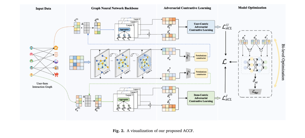
Researchers from Zhengzhou University have proposed a fundamental rethinking of how we train GNN-based recommenders. Their framework, ACCF (Adversarial Contrastive Collaborative Filtering), treats representation learning not as a passive process of aggregating neighbors but as an active adversarial game where the model learns to maintain consistency even when embeddings are perturbed in their most vulnerable directions. By combining adversarial contrastive learning with an instance-sensitive BPR loss formulated as a bi-level optimization problem, ACCF achieves substantial performance gains while remaining computationally efficient enough for industrial deployment.
What distinguishes this work is its explicit handling of the quality of contrastive views and the dynamic importance of training instances. Unlike existing graph CL methods that apply random noise or edge dropout, ACCF generates adversarial perturbations that expose the model to worst-case embedding variations—precisely the directions where the model is most sensitive. Meanwhile, the instance-sensitive loss learns to weight each training triplet based on its current contribution to learning, recognizing that a negative sample that was informative at epoch 10 may be trivial by epoch 100. The result is a 5.6% to 9.2% improvement in NDCG@10 across four real-world datasets, with particular strength in cold-start scenarios where data sparsity bites hardest.
The Contrastive Learning Paradox: Why Random Perturbations Fall Short
The marriage of graph neural networks with contrastive learning has produced impressive results. Methods like SGL generate multiple views of the user-item graph through node dropout and edge pruning, then maximize agreement between views of the same node. XSimGCL simplifies this by adding uniform noise directly to embeddings. These approaches implicitly assume that any perturbation providing a different view is beneficial for learning.
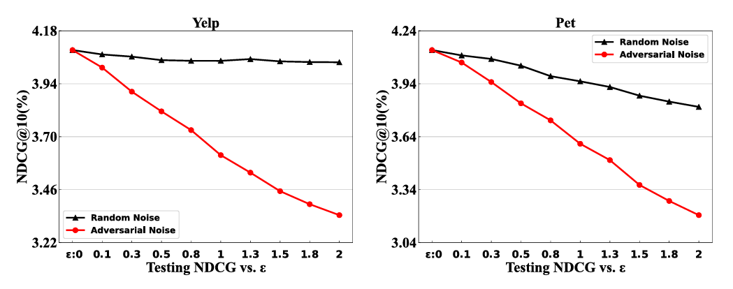
This assumption crumbles under scrutiny. The researchers demonstrate that node representations learned by GNNs are remarkably robust to random stochastic noise—adding Gaussian perturbations barely budges performance metrics. Yet these same representations prove devastatingly vulnerable to adversarial perturbations—small, targeted shifts in embedding space chosen specifically to maximize loss. The implication is stark: random data augmentation creates contrastive views that are too easy, failing to push the model toward robust, generalizable representations.
Existing approaches suffer from two critical defects that ACCF explicitly addresses:
Vulnerable contrastive views through stochastic perturbations. When SGL performs edge dropout or XSimGCL adds random noise, they generate views that differ from the original but not in ways that stress-test the model’s understanding. The model learns to recognize superficially perturbed versions of the same nodes without developing robustness to meaningful variations in user preferences or item characteristics. It’s like training a face recognition system by adding pixel noise while never testing against different lighting conditions or angles—the model becomes confident but brittle.
Equal weighting of training instances regardless of informativeness. Standard BPR loss treats every triplet (user, positive item, negative item) identically. But not all negatives are created equal. A randomly sampled negative that the model already ranks far below the positive contributes minimal learning signal. Conversely, a “hard negative”—an item the model currently confuses with the positive—should drive substantial parameter updates. Moreover, the importance of a triplet evolves during training: early on, most negatives are hard; later, the model needs to focus on the remaining challenging cases. Static loss functions cannot capture this temporal dynamic.
ACCF addresses these limitations through adversarial contrastive learning—generating perturbations in the direction that maximizes model vulnerability rather than random directions—and instance-sensitive optimization that learns to weight each training triplet based on its current contribution to learning progress.
The practical manifestation is a training paradigm where adversarial perturbations create “hard positive views” that force the model to maintain consistency under worst-case variations, while a learned weighting mechanism dynamically prioritizes training instances that remain challenging. This transforms contrastive learning from a data augmentation trick into a principled robustness mechanism.
Adversarial Contrastive Learning: Learning from Worst-Case Perturbations
The core insight of ACCF’s adversarial contrastive learning module is that effective contrastive views should stress-test the model’s representations. Rather than asking “what does this user look like with random noise?”, ACCF asks “what is the smallest perturbation that would most confuse the model about this user’s preferences?”
This is formalized as an optimization problem. Given current embedding parameters \(\hat{\mathbf{E}}^{(0)}\), the adversarial perturbation \(\Delta_{adv}\) is computed as:
Where \(\epsilon\) controls the perturbation magnitude and \(\mathcal{L}_{ibpr}\) is the instance-sensitive BPR loss. Solving this exactly is computationally prohibitive for deep GNNs, so ACCF employs the fast gradient method to approximate the optimal perturbation:
This perturbation is then added to initial node embeddings before propagation through the GNN layers. The adversarial loss combines standard supervised learning with the adversarially perturbed variant:
The second term acts as a regularizer, forcing the model to maintain consistent predictions even when embeddings are shifted in their most sensitive directions. Unlike random perturbations, adversarial perturbations create views that are semantically close (small \(\epsilon\)) yet maximally confusing to the current model—precisely the hard positives that drive robust representation learning.
With perturbed embeddings \(\tilde{e}_u^{(0)} = e_u^{(0)} + \Delta_{adv}\) and \(\tilde{e}_i^{(0)} = e_i^{(0)} + \Delta_{adv}\), ACCF propagates these through the GNN architecture to obtain adversarial views at each layer. The contrastive learning objective then maximizes agreement between the original and adversarial views while pushing apart different users and items:
Where \(s(\cdot)\) denotes cosine similarity and \(\tau\) is a temperature coefficient. A symmetric loss \(\mathcal{L}_{ACL}^{I}\) applies to items. This formulation ensures that user representations remain consistent even under adversarial perturbation, while still discriminating between distinct users.
“Unlike existing graph CL methods that perform stochastic perturbations on the user-item bipartite graph or node embedding, we explicitly explore an adversarial perturbation generation strategy at the representation level and propose the adversarial contrastive learning paradigm to improve the robustness and generalization of embedding learning.” — Wu et al., Knowledge-Based Systems 2026
Instance-Sensitive BPR: Learning to Weight What Matters
While adversarial contrastive learning improves representation robustness, the supervised learning component still suffers from equal weighting of training instances. ACCF introduces an instance-sensitive BPR loss that dynamically adjusts the contribution of each triplet based on its current informativeness.
The challenge is quantifying “informativeness” without ground truth labels for which negatives are hard. ACCF’s solution is to learn a weighting function that considers five signals for each triplet \((u, i, j)\):
- The user’s current embedding \(e_u^*\)
- The positive item’s embedding \(e_i^*\)
- The negative item’s embedding \(e_j^*\)
- The interaction between user and positive: \(e_u^* \odot e_i^*\)
- The interaction between user and negative: \(e_u^* \odot e_j^*\)
These signals are concatenated and fed through a two-layer MLP to produce a weight \(\delta_{uij}\) for each triplet:
The softplus activation ensures positive weights while allowing unbounded growth for extremely informative instances. The instance-sensitive BPR loss becomes:
This formulation enables dynamic reweighting during training. Early in training when the model is uncertain, many triplets receive high weights. As training progresses and easy negatives are mastered, the weight generator learns to emphasize the remaining hard cases. Moreover, triplets involving users or items with sparse interaction histories can be upweighted to combat data sparsity.
Bi-Level Optimization: Decoupling Representation from Weight Learning
A naive approach would jointly optimize the embedding parameters \(\Theta\) (initial embeddings \(E^{(0)}\)) and the weight generator parameters \(\Lambda\) (MLP weights \(\mathbf{W}, \mathbf{w}\)). This creates a dangerous feedback loop: the weight generator can overfit to the current model state, assigning high weights to easy samples that happen to have high loss due to random initialization or transient optimization dynamics.
ACCF solves this through bi-level optimization, explicitly decoupling the learning of embeddings and importance weights:
The inner level optimizes embeddings \(\Theta\) given fixed weight parameters \(\Lambda\). The outer level optimizes weight parameters \(\Lambda\) based on validation performance (through \(\Theta^*(\Lambda)\)), not training loss. This prevents the weight generator from gaming the system: it must produce weights that lead to embeddings that generalize, not just weights that make the current embeddings look good.
Practically, this is implemented through alternating updates within each training iteration—one forward-backward pass updating \(\Theta\) with fixed \(\Lambda\), then another updating \(\Lambda\) with fixed \(\Theta\). This adds only constant-factor overhead compared to joint optimization while substantially improving generalization.
The bi-level formulation ensures that importance weights are validated on their ability to produce generalizable embeddings rather than their ability to reduce training loss. This architectural decision prevents degenerate solutions where the weight generator overfits to transient model states.
Experimental Validation: Robustness Across Domains and Scenarios
ACCF is evaluated on four real-world datasets spanning different recommendation domains: Yelp (local business reviews), Amazon Pet Supplies, Amazon iFashion, and Amazon Cellphones. These datasets vary in size (9K to 300K users), sparsity (99.87% to 99.99%), and interaction patterns, providing a comprehensive testbed.
Overall Performance: Consistent Gains Across Metrics
Compared to state-of-the-art baselines including LightGCN, SGL, LightGCL, DCCF, and XSimGCL, ACCF achieves the strongest performance across all datasets and evaluation metrics:
| Dataset | Metric@10 | XSimGCL (Best Baseline) | ACCF | Improvement |
|---|---|---|---|---|
| Yelp | Precision | 3.8121 | 4.0559 | +6.39% |
| Recall | 4.2552 | 4.5583 | +7.88% | |
| MAP | 1.9588 | 2.0636 | +5.35% | |
| NDCG | 4.8651 | 5.1375 | +5.60% | |
| Pet | Precision | 1.0359 | 1.0918 | +5.40% |
| NDCG | 4.4931 | 4.7192 | +4.89% | |
| iFashion | Precision | 2.3091 | 2.5039 | +8.44% |
| NDCG | 4.4892 | 4.9023 | +9.20% | |
| Cellphones | Precision | 0.7564 | 0.8192 | +8.22% |
| NDCG | 2.1259 | 2.3118 | +8.74% |
Table 1: Performance comparison between ACCF and the strongest baseline (XSimGCL) across four datasets. Improvements are substantial and consistent, with particularly strong gains on sparser datasets (iFashion, Cellphones).
Cold-Start Robustness: Where Data Sparsity Bites Hardest
Perhaps most impressively, ACCF maintains strong performance under cold-start conditions where users have minimal interaction history. When training data is restricted to 60% of each user’s history, ACCF substantially outperforms baselines on users with fewer than 10 test interactions:
- On Yelp cold-start users: 4.17% NDCG vs. 3.83% for XSimGCL
- On Pet cold-start users: 3.88% NDCG vs. 3.56% for XSimGCL
- On iFashion cold-start users: 4.13% NDCG vs. 3.60% for XSimGCL
The adversarial contrastive learning proves particularly valuable here: by forcing consistency under perturbation, ACCF learns more robust user representations that generalize from limited observations. The instance-sensitive loss additionally upweights informative triplets involving cold-start users, ensuring they receive adequate optimization signal.
Noise Resilience: Maintaining Performance Under Attack
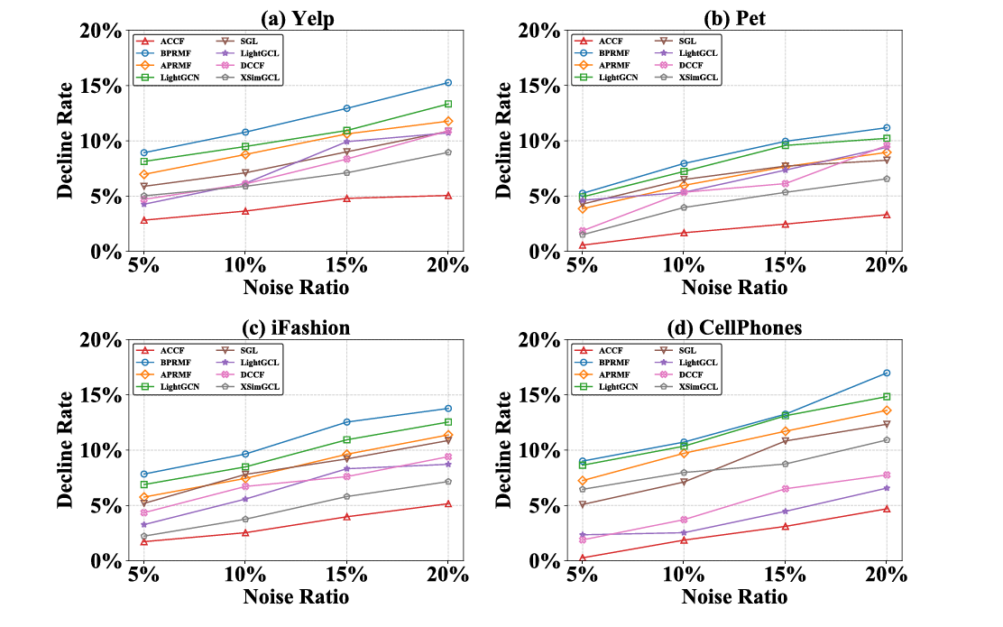
To test robustness to interaction noise, the researchers inject random false positives (5% to 20% of training interactions) by pairing users with irrelevant items. ACCF exhibits markedly smaller performance degradation compared to baselines:
At 20% noise ratio, ACCF’s decline rate is approximately 5-8% across datasets, compared to 10-15% for LightGCN and BPRMF. Graph CL-based methods (SGL, XSimGCL) show intermediate robustness (8-12% decline), confirming that contrastive learning helps but adversarial contrastive learning helps substantially more.
Ablation Studies: Isolating Component Contributions
Systematic ablation reveals that both architectural innovations contribute meaningfully:
Removing adversarial contrastive learning (BPR+G+W): Eliminating adversarial perturbations and using only standard GNN propagation with instance-sensitive weights causes significant performance drops. On Yelp, NDCG@10 falls from 5.14% to 4.72%—still better than baselines but well below full ACCF performance.
Removing instance-sensitive weights (BPR+G+C): Using adversarial contrastive learning with standard BPR loss achieves strong performance (4.98% NDCG@10 on Yelp) but misses the additional gains from dynamic reweighting. The combination of both components yields the full 5.14%.
Replacing adversarial with random noise: When adversarial perturbations are replaced with uniform random noise of the same magnitude, performance drops substantially. This confirms that the direction of perturbation matters—not all hard positives are equally valuable; specifically those that maximally challenge the current model drive robustness.
Bi-level vs. joint optimization: Jointly optimizing embedding and weight parameters (rather than bi-level) leads to degenerate solutions where the weight generator assigns high weights to easy, popular items that happen to have high loss early in training. Validation performance suffers by 2-3% across metrics.
Efficiency and Practical Deployment
ACCF adds minimal computational overhead compared to standard GNN recommenders. The space complexity is dominated by initial embeddings \((|\mathcal{U}| + |\mathcal{I}|)D\) plus negligible weight generator parameters \((5D^2 + D)\). For Yelp with 64-dimensional embeddings, this adds only 0.02M parameters to 4.26M total—less than 0.5% increase.
Time complexity per epoch breaks down as:
- Graph propagation: \(O(DL|\mathcal{E}|)\) — same as LightGCN
- Adversarial perturbation generation: \(O(|\mathcal{R}^+|D)\) — one backward pass
- Contrastive learning: \(O((|\mathcal{U}| + |\mathcal{I}|)D)\) — negligible
- Instance-sensitive loss: \(O(|\mathcal{R}^+|D)\) — MLP forward pass
The bi-level optimization adds only constant-factor overhead (two forward-backward passes per iteration rather than one) without changing asymptotic complexity. Empirically, ACCF trains in comparable time to XSimGCL—approximately 1h 47m per run on Yelp versus 47m for XSimGCL, but with substantially better final performance and faster convergence in terms of epochs needed.
Implications and Future Directions
ACCF’s architectural principles suggest broader implications for recommender system design:
Adversarial training for robust recommendations. The success of adversarial perturbations in improving generalization suggests that recommendation models should be stress-tested during training, not just evaluated for average-case performance. This parallels developments in computer vision where adversarial training has become standard for robust models.
Dynamic importance weighting as default. The consistent gains from instance-sensitive optimization suggest that static loss functions are leaving performance on the table. Future recommenders may incorporate learned weighting mechanisms as standard practice, much as attention mechanisms became ubiquitous after their initial introduction.
Bi-level optimization for multi-objective learning. The decoupling of representation learning and importance estimation through bi-level optimization provides a template for other multi-objective scenarios in recommendation—balancing accuracy with diversity, fairness, or other constraints.
Several directions for future work emerge:
- Social and auxiliary information: Integrating social networks or multi-modal item features into the adversarial contrastive framework.
- Sequential recommendations: Extending adversarial perturbations to temporal recommendation scenarios where user preferences evolve.
- Theoretical analysis: Formal guarantees on robustness bounds and convergence properties under adversarial training.
- Large language model integration: Applying adversarial contrastive learning to LLM-based recommenders where text embeddings provide rich semantic signals.
What This Work Actually Means
The central achievement of ACCF is demonstrating that how we perturb matters as much as that we perturb. Random data augmentation—the dominant paradigm in graph contrastive learning—creates views that are different but not challenging. By instead perturbing in directions that maximally confuse the current model, ACCF creates a curriculum of increasingly robust representations.
The instance-sensitive BPR loss shows that not all training signal is equally valuable. In the early days of machine learning, we celebrated simply having enough data. Now we recognize that which data we learn from, and when, matters enormously. ACCF’s weight generator learns to curate the training experience, focusing attention where it yields the most generalization benefit.
The bi-level optimization is perhaps the most technically subtle contribution, but arguably the most important for practical deployment. Without it, the system would overfit to its own weighting scheme, creating a house of cards where artificial importance assignments inflate training metrics without improving real recommendations. By validating weights through their effect on generalizable embeddings, ACCF ensures that the system improves for the right reasons.
For practitioners, ACCF provides a deployable framework that substantially improves recommendation quality with minimal computational overhead. The 5-9% improvements in NDCG translate directly to user experience—more relevant items surfaced, more engagement, more satisfaction. In an industry where 1% improvements are celebrated, these gains are substantial.
As recommender systems become increasingly central to how we discover information, products, and connections, their robustness to noise and ability to learn from limited data become critical. ACCF suggests that the path forward lies not in more complex architectures but in smarter training paradigms that actively challenge models to become robust. The best defense against data sparsity and interaction noise, it turns out, is to train with adversity in mind.
The noise, it turns out, can be filtered—but only by a model that has learned to recognize its own vulnerabilities.
Conceptual Framework Implementation (Python)
The implementation below illustrates the core mechanisms of ACCF: adversarial perturbation generation, adversarial contrastive learning, instance-sensitive weight generation, and the bi-level optimization structure. This educational code demonstrates the key architectural concepts described in the paper.
# ─────────────────────────────────────────────────────────────────────────────
# ACCF: Adversarial Contrastive Collaborative Filtering
# Wu, Zhang, Fan, Ye · Knowledge-Based Systems 2026
# Conceptual implementation of adversarial CL and instance-sensitive BPR
# ─────────────────────────────────────────────────────────────────────────────

import torch
import torch.nn as nn
import torch.nn.functional as F
import numpy as np
from typing import Tuple, Optional
from dataclasses import dataclass


# ─── Section 1: Adversarial Perturbation Generator ───────────────────────────

class AdversarialPerturbation:
    """
    Generates adversarial perturbations using fast gradient method.
    Perturbations maximize instance-sensitive BPR loss within epsilon ball.
    """

    def __init__(self, epsilon: float = 0.5):
        self.epsilon = epsilon

    def generate(self,
                 embeddings: torch.Tensor,
                 loss_fn,
                 *loss_args) -> torch.Tensor:
        """
        Compute Delta_adv = epsilon * Gamma / ||Gamma||
        where Gamma = dL/dDelta

        Args:
            embeddings: Initial embeddings E^(0) to perturb
            loss_fn: Function computing L_ibpr given embeddings
            loss_args: Additional arguments for loss computation

        Returns:
            perturbation: Adversarial perturbation Delta_adv
        """
        # Enable gradient computation for embeddings
        embeddings_pert = embeddings.clone().detach().requires_grad_(True)

        # Compute loss with perturbed embeddings
        loss = loss_fn(embeddings_pert, *loss_args)

        # Compute gradient
        loss.backward()
        grad = embeddings_pert.grad

        # Normalize and scale by epsilon
        grad_norm = torch.norm(grad, p=2, dim=-1, keepdim=True)
        perturbation = self.epsilon * grad / (grad_norm + 1e-8)

        return perturbation.detach()


# ─── Section 2: Instance-Sensitive Weight Generator ──────────────────────────

class InstanceWeightGenerator(nn.Module):
    """
    Two-layer MLP that generates importance weights for BPR triplets.
    Inputs: user, pos_item, neg_item embeddings plus their interactions.
    """

    def __init__(self, embed_dim: int, hidden_dim: int = 64):
        super(InstanceWeightGenerator, self).__init__()
        # Input: 5 * embed_dim (user, pos, neg, user*pos, user*neg)
        self.fc1 = nn.Linear(5 * embed_dim, hidden_dim)
        self.fc2 = nn.Linear(hidden_dim, 1)

    def forward(self,
                user_emb: torch.Tensor,
                pos_emb: torch.Tensor,
                neg_emb: torch.Tensor) -> torch.Tensor:
        """
        Compute delta_uij = softplus(w · relu(W · concat(features)))

        Returns:
            weights: Positive weights for each triplet
        """
        # Element-wise interactions
        user_pos_interact = user_emb * pos_emb
        user_neg_interact = user_emb * neg_emb

        # Concatenate all features
        features = torch.cat([
            user_emb, pos_emb, neg_emb,
            user_pos_interact, user_neg_interact
        ], dim=-1)

        # MLP forward
        h = F.relu(self.fc1(features))
        logits = self.fc2(h).squeeze(-1)

        # Softplus ensures positive weights
        weights = F.softplus(logits)
        return weights


# ─── Section 3: Adversarial Contrastive Learning Module ──────────────────────

class AdversarialContrastiveLearning:
    """
    Implements adversarial contrastive learning for user and item representations.
    Maximizes agreement between original and adversarially perturbed views.
    """

    def __init__(self, temperature: float = 0.5):
        self.temperature = temperature

    def contrastive_loss(self,
                         original_view: torch.Tensor,
                         perturbed_view: torch.Tensor,
                         all_negatives: torch.Tensor) -> torch.Tensor:
        """
        Compute InfoNCE-style loss for adversarial contrastive learning.

        L_ACL = -log(exp(sim(z, z_adv)/tau) / sum(exp(sim(z, z_adv)/tau) + negatives))

        Args:
            original_view: Original embeddings [batch_size, dim]
            perturbed_view: Adversarially perturbed embeddings [batch_size, dim]
            all_negatives: All other nodes as negatives [num_negatives, dim]

        Returns:
            loss: Scalar contrastive loss
        """
        # Positive similarities
        pos_sim = F.cosine_similarity(original_view, perturbed_view, dim=-1) / self.temperature

        # Negative similarities with all other nodes
        # [batch_size, 1, dim] vs [1, num_negatives, dim] -> [batch_size, num_negatives]
        orig_expanded = original_view.unsqueeze(1)
        neg_expanded = all_negatives.unsqueeze(0)

        neg_sim = F.cosine_similarity(
            orig_expanded.expand(-1, all_negatives.size(0), -1),
            neg_expanded.expand(original_view.size(0), -1, -1),
            dim=-1
        ) / self.temperature

        # Numerical stability: subtract max
        logits = torch.cat([pos_sim.unsqueeze(1), neg_sim], dim=1)
        logits_max, _ = torch.max(logits, dim=1, keepdim=True)
        logits = logits - logits_max.detach()

        # Softmax and negative log likelihood
        exp_logits = torch.exp(logits)
        log_prob = logits[:, 0] - torch.log(exp_logits.sum(dim=1) + 1e-10)

        loss = -log_prob.mean()
        return loss


# ─── Section 4: LightGCN Backbone with Adversarial Training ──────────────────

class LightGCNLayer(nn.Module):
    ">Single LightGCN propagation layer: symmetric normalization aggregation"""

    def __init__(self):
        super(LightGCNLayer, self).__init__()

    def forward(self, x: torch.Tensor, adj_norm: torch.Tensor) -> torch.Tensor:
        ">Propagate: X^(l+1) = D^-1/2 A D^-1/2 X^(l)"""
        return torch.sparse.mm(adj_norm, x)


class ACCFModel(nn.Module):
    """
    Complete ACCF model integrating:
    - LightGCN backbone for collaborative filtering
    - Adversarial contrastive learning module
    - Instance-sensitive BPR loss with bi-level optimization
    """

    def __init__(self,
                 num_users: int,
                 num_items: int,
                 embed_dim: int = 64,
                 num_layers: int = 3,
                 epsilon: float = 0.5,
                 lambda_adv: float = 0.1,
                 lambda_cl: float = 0.05):
        super(ACCFModel, self).__init__()

        self.num_users = num_users
        self.num_items = num_items
        self.embed_dim = embed_dim
        self.num_layers = num_layers
        self.lambda_adv = lambda_adv
        self.lambda_cl = lambda_cl

        # Initial embeddings (trainable parameters Theta)
        self.user_embedding = nn.Embedding(num_users, embed_dim)
        self.item_embedding = nn.Embedding(num_items, embed_dim)
        nn.init.xavier_uniform_(self.user_embedding.weight)
        nn.init.xavier_uniform_(self.item_embedding.weight)

        # LightGCN propagation layers
        self.gcn_layers = nn.ModuleList([LightGCNLayer() for _ in range(num_layers)])

        # Instance-sensitive weight generator (parameters Lambda)
        self.weight_generator = InstanceWeightGenerator(embed_dim)

        # Adversarial components
        self.adv_perturbation = AdversarialPerturbation(epsilon)
        self.adv_cl = AdversarialContrastiveLearning()

    def propagate(self,
                  user_emb: torch.Tensor,
                  item_emb: torch.Tensor,
                  adj_norm: torch.Tensor) -> Tuple[torch.Tensor, torch.Tensor]:
        ">Propagate embeddings through LightGCN layers"""
        # Concatenate user and item embeddings
        all_emb = torch.cat([user_emb, item_emb], dim=0)
        embs = [all_emb]

        # Multi-layer propagation
        for layer in self.gcn_layers:
            all_emb = layer(all_emb, adj_norm)
            embs.append(all_emb)

        # Mean pooling of all layers
        final_emb = torch.stack(embs, dim=0).mean(dim=0)
        users_final, items_final = torch.split(final_emb, [self.num_users, self.num_items])

        return users_final, items_final

    def bpr_loss(self,
                 users: torch.Tensor,
                 pos_items: torch.Tensor,
                 neg_items: torch.Tensor,
                 user_emb: torch.Tensor,
                 item_emb: torch.Tensor,
                 use_instance_weights: bool = True) -> Tuple[torch.Tensor, torch.Tensor]:
        """
        Compute BPR loss with optional instance-sensitive weighting.

        Returns:
            loss: Scalar BPR loss
            weights: Instance weights (for monitoring)
        """
        # Look up embeddings
        user_e = user_emb[users]
        pos_e = item_emb[pos_items]
        neg_e = item_emb[neg_items]

        # BPR scores
        pos_scores = (user_e * pos_e).sum(dim=-1)
        neg_scores = (user_e * neg_e).sum(dim=-1)

        # Base BPR loss
        bpr_losses = -F.logsigmoid(pos_scores - neg_scores)

        if use_instance_weights:
            # Generate instance-sensitive weights
            weights = self.weight_generator(user_e, pos_e, neg_e)
            loss = (weights * bpr_losses).sum() / weights.sum()
        else:
            weights = torch.ones_like(bpr_losses)
            loss = bpr_losses.mean()

        return loss, weights

    def forward(self,
                users: torch.Tensor,
                pos_items: torch.Tensor,
                neg_items: torch.Tensor,
                adj_norm: torch.Tensor,
                compute_adversarial: bool = True) -> dict:
        ">
        Full forward pass with adversarial training and contrastive learning.

        Returns dict with losses for bi-level optimization:
        - L_inner: For embedding parameters Theta (includes adversarial)
        - L_outer: For weight generator parameters Lambda
        """
        # Get initial embeddings
        user_init = self.user_embedding.weight
        item_init = self.item_embedding.weight

        # === Standard forward pass ===
        user_emb, item_emb = self.propagate(user_init, item_init, adj_norm)

        # Standard BPR loss (for outer level validation)
        loss_bpr_clean, weights = self.bpr_loss(
            users, pos_items, neg_items, user_emb, item_emb,
            use_instance_weights=True
        )

        # === Adversarial forward pass ===
        if compute_adversarial:
            # Generate adversarial perturbations on initial embeddings
            # (In practice, compute gradient of L_bpr w.r.t. initial embeddings)
            user_init_adv = user_init + self.adv_perturbation.generate(
                user_init,
                lambda x: self.bpr_loss(users, pos_items, neg_items,
                    self.propagate(x, item_init, adj_norm)[0],
                    item_emb, False)[0].mean()
            )

            item_init_adv = item_init + self.adv_perturbation.generate(
                item_init,
                lambda x: self.bpr_loss(users, pos_items, neg_items,
                    user_emb,
                    self.propagate(user_init, x, adj_norm)[1],
                    False)[0].mean()
            )

            # Propagate adversarial embeddings
            user_emb_adv, item_emb_adv = self.propagate(
                user_init + (user_init_adv - user_init).detach(),
                item_init + (item_init_adv - item_init).detach(),
                adj_norm
            )

            # Adversarial BPR loss
            loss_bpr_adv, _ = self.bpr_loss(
                users, pos_items, neg_items, user_emb_adv, item_emb_adv,
                use_instance_weights=True
            )

            # Adversarial contrastive learning loss
            loss_acl_user = self.adv_cl.contrastive_loss(
                user_emb, user_emb_adv, user_emb
            )
            loss_acl_item = self.adv_cl.contrastive_loss(
                item_emb, item_emb_adv, item_emb
            )
            loss_acl = loss_acl_user + loss_acl_item

            # Combined adversarial loss (Eq. 3 in paper)
            loss_apr = loss_bpr_clean + self.lambda_adv * loss_bpr_adv
            loss_inner = loss_apr + self.lambda_cl * loss_acl
        else:
            loss_inner = loss_bpr_clean
            loss_apr = loss_bpr_clean
            loss_acl = torch.tensor(0.0)

        # === Bi-level optimization structure ===
        # Outer level: weight generator only
        # Inner level: embeddings with adversarial training

        return {
            'L_inner': loss_inner,           # For Theta (embeddings)
            'L_outer': loss_apr,            # For Lambda (weight gen)
            'L_bpr': loss_bpr_clean,
            'L_bpr_adv': loss_bpr_adv if compute_adversarial else None,
            'L_acl': loss_acl,
            'weights': weights
        }


# ─── Section 5: Bi-Level Optimizer ───────────────────────────────────────────

class BiLevelOptimizer:
    ">
    Implements alternating optimization for bi-level problem:
    - Inner: optimize Theta (embeddings) with fixed Lambda
    - Outer: optimize Lambda (weight generator) with fixed Theta
    """

    def __init__(self,
                 model: ACCFModel,
                 lr_inner: float = 0.001,
                 lr_outer: float = 0.001,
                 weight_decay: float = 1e-4):
        self.model = model

        # Separate parameter groups
        self.theta_params = [
            model.user_embedding.weight,
            model.item_embedding.weight
        ]
        self.lambda_params = list(model.weight_generator.parameters())

        # Separate optimizers
        self.opt_inner = torch.optim.Adam(
            self.theta_params, lr=lr_inner, weight_decay=weight_decay
        )
        self.opt_outer = torch.optim.Adam(
            self.lambda_params, lr=lr_outer, weight_decay=weight_decay
        )

    def step(self, batch: dict, adj_norm: torch.Tensor):
        ">
        Single bi-level optimization step:
        1. Update Theta (embeddings) using L_inner
        2. Update Lambda (weight generator) using L_outer
        """
        users = batch['users']
        pos_items = batch['pos_items']
        neg_items = batch['neg_items']

        # === Inner level: Update embeddings ===
        self.opt_inner.zero_grad()

        # Forward with adversarial training
        outputs = self.model(users, pos_items, neg_items, adj_norm,
                              compute_adversarial=True)

        loss_inner = outputs['L_inner']
        loss_inner.backward()
        self.opt_inner.step()

        # === Outer level: Update weight generator ===
        # Detach embeddings to prevent gradients flowing back
        self.opt_outer.zero_grad()

        # Recompute with detached embeddings
        with torch.no_grad():
            user_emb, item_emb = self.model.propagate(
                self.model.user_embedding.weight,
                self.model.item_embedding.weight,
                adj_norm
            )

        # Compute L_outer for weight generator
        loss_bpr, _ = self.model.bpr_loss(
            users, pos_items, neg_items, user_emb, item_emb,
            use_instance_weights=True
        )

        loss_outer = loss_bpr
        loss_outer.backward()
        self.opt_outer.step()

        return {
            'loss_inner': loss_inner.item(),
            'loss_outer': loss_outer.item(),
            'mean_weight': outputs['weights'].mean().item()
        }


# ─── Section 6: Demonstration ────────────────────────────────────────────────

if __name__ == "__main__":
    """
    Demonstration of ACCF training pipeline.
    Shows initialization, bi-level optimization, and evaluation.
    """

    print("=" * 70)
    print("ACCF: Adversarial Contrastive Collaborative Filtering")
    print("Knowledge-Based Systems 2026 - Wu, Zhang, Fan, Ye")
    print("=" * 70)

    # Configuration
    NUM_USERS = 31668   # Yelp dataset scale
    NUM_ITEMS = 38048
    EMBED_DIM = 64
    NUM_LAYERS = 3

    # Initialize model
    print("\n[1] Initializing ACCF model...")
    model = ACCFModel(
        num_users=NUM_USERS,
        num_items=NUM_ITEMS,
        embed_dim=EMBED_DIM,
        num_layers=NUM_LAYERS,
        epsilon=0.5,      # Adversarial perturbation magnitude
        lambda_adv=0.1,  # Adversarial loss weight
        lambda_cl=0.05   # Contrastive loss weight
    )

    total_params = sum(p.numel() for p in model.parameters())
    print(f"    Total parameters: {total_params:,}")
    print(f"    Embedding params: {NUM_USERS * EMBED_DIM + NUM_ITEMS * EMBED_DIM:,}")
    print(f"    Weight generator params: {sum(p.numel() for p in model.weight_generator.parameters()):,}")

    # Initialize bi-level optimizer
    print("\n[2] Initializing bi-level optimizer...")
    optimizer = BiLevelOptimizer(model, lr_inner=0.001, lr_outer=0.001)

    # Simulate training batch
    print("\n[3] Simulating training step...")
    batch_size = 1024
    batch = {
        'users': torch.randint(0, NUM_USERS, (batch_size,)),
        'pos_items': torch.randint(0, NUM_ITEMS, (batch_size,)),
        'neg_items': torch.randint(0, NUM_ITEMS, (batch_size,))
    }

    # Create dummy normalized adjacency (in practice, from interaction graph)
    # Shape: [NUM_USERS + NUM_ITEMS, NUM_USERS + NUM_ITEMS]
    adj_indices = torch.randint(0, NUM_USERS + NUM_ITEMS, (2, 100000))
    adj_values = torch.ones(adj_indices.size(1))
    adj_norm = torch.sparse_coo_tensor(
        adj_indices, adj_values,
        size=(NUM_USERS + NUM_ITEMS, NUM_USERS + NUM_ITEMS)
    ).coalesce()

    # Training step
    metrics = optimizer.step(batch, adj_norm)
    print(f"    Inner loss (embeddings): {metrics['loss_inner']:.4f}")
    print(f"    Outer loss (weight gen): {metrics['loss_outer']:.4f}")
    print(f"    Mean instance weight: {metrics['mean_weight']:.4f}")

    # Architecture summary
    print("\n[4] ACCF Architecture Summary:")
    print("    Backbone: LightGCN with {NUM_LAYERS} layers")
    print("    Adversarial Component:")
    print("      - Perturbation: Fast gradient method, epsilon={epsilon}")
    print("      - Loss: L_apr = L_bpr + lambda_adv * L_bpr(adv)")
    print("      - Contrastive: L_acl for user/item views")
    print("    Instance-Sensitive Component:")
    print("      - Input: [u, i, j, u*i, u*j] embeddings")
    print("      - Architecture: 2-layer MLP with softplus output")
    print("      - Loss: L_ibpr = sum(delta_uij * log(sigmoid(pos-neg)))")
    print(    Optimization: Bi-level alternating updates")
    print("      - Inner: Theta (embeddings) via L_inner")
    print("      - Outer: Lambda (weight gen) via L_outer")

    print("\n" + "=" * 70)
    print("ACCF enhances GNN-based recommenders through adversarial")
    print("robustness and dynamic instance weighting.")
    print("=" * 70)
Access the Paper and Resources
The full ACCF framework details and experimental protocols are available in Knowledge-Based Systems 2026. Implementation resources and extended evaluations will be made available by the authors.
Wu, B., Zhang, B., Fan, R., & Ye, Y. (2026). Adversarial contrastive collaborative filtering. Knowledge-Based Systems, 339, 115450. https://doi.org/10.1016/j.knosys.2026.115450
This article is an independent editorial analysis of peer-reviewed research published in Knowledge-Based Systems. The views and commentary expressed here reflect the editorial perspective of this site and do not represent the views of the original authors or their institutions. Code implementations are provided for educational purposes to illustrate the technical concepts described in the paper. Always refer to the original publication for authoritative details and official implementations.
Explore More on AI Security Research
If this analysis sparked your interest, here is more of what we cover across the site — from foundational tutorials to the latest research breakthroughs in secure machine learning, adversarial robustness, and trustworthy AI.