MSDN++: The Zero-Shot Learner That Asks “Why?” Before It Answers
Researchers from Huazhong University of Science and Technology built a network that recognises objects it has never seen before — by first applying a causal intervention test to check whether its attention maps are actually paying attention to the right things, not just producing plausible-looking activations.
Imagine a medical AI that can identify a rare disease it was never trained on — simply because it learned what “inflamed tissue” and “abnormal cell clustering” look like in general, and can transfer that knowledge using shared semantic attributes. That is zero-shot learning’s promise. The reason it is hard to deliver on is that most models learn the wrong visual patterns while appearing to learn the right ones. MSDN++ fixes this with a philosophical upgrade: instead of just asking “what does this look like?” it asks “what would happen to my answer if I removed this visual cue entirely?” That causal question changes everything.
The Core Problem: Spurious Attention
The dominant approach to zero-shot learning has been attention-based: use attribute descriptions like “bill color yellow” or “has wings” as queries to focus the model on the image regions relevant to each attribute, then match those attended features against class prototypes. This works well in theory. In practice, something fundamental goes wrong.
Attention maps are trained with a simple loss — the final classification must be correct — but nothing explicitly ensures the attention was causally responsible for the correct answer. A model can achieve high training accuracy while attending to the wrong image regions, because training data contains systematic biases. If every bird image with a yellow bill also has a distinctive background or body shape, the model may learn to link the attribute “bill color yellow” to the background rather than the bill. The attention looks plausible, accuracy is high on training classes, and then the model fails badly on unseen classes that do not share those dataset biases.
There is a second failure mode: almost all prior ZSL attention methods are unidirectional. They learn to attend from attributes to image regions — asking “where in the image is this attribute?” — but never ask the reverse: “given this image region, which attributes does it provide evidence for?” These two directions are complementary, not redundant, and ignoring one loses calibrating information that could correct errors in the other.
Prior attention-based ZSL methods suffer from spurious correlations — attention maps driven by dataset bias rather than genuine causal structure — and unidirectional attention that leaves the complementary visual→attribute direction unexplored. MSDN++ addresses both with causal intervention and bidirectional mutual distillation.
Architecture: Two Sub-Nets Running in Opposite Directions
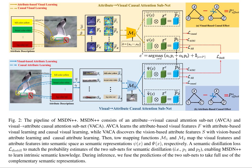
MSDN++ is built around two complementary attention sub-networks. The first, AVCA (Attribute→Visual Causal Attention), asks: for each semantic attribute, which image regions are most relevant? The second, VACA (Visual→Attribute Causal Attention), runs the problem in the opposite direction: for each image region, which attribute descriptions does it most support? Both sub-nets share a ResNet101 visual backbone and GloVe attribute embeddings, but learn entirely different attention patterns.
MSDN++ PIPELINE
══════════════════════════════════════════════════════════

Image → ResNet101 → V = {v1,...,vR}     (R=196 regions, 14×14)
Attributes → GloVe → A = {a1,...,aK}   (K attributes per class)

┌─────────────── AVCA Sub-Net ───────────────────────────┐
│  β^r_k = softmax( a_k^T · W1 · v_r )     [Eq. 1]     │
│  F_k = Σ_r β^r_k · v_r                   [Eq. 2]     │
│  ψ_k = a_k^T · W2 · F_k                  [Eq. 3]     │
│  p1 = ψ(x) · z^c      (observation)      [Eq. 4]     │
│  ──── Causal ────                                      │
│  do(β = β̄): replace attention with random            │
│  P^v_effect = P(β,X) - P(do(β=β̄),X)     [Eq. 6]     │
└────────────────────────────────────────────────────────┘
         ↕ L_distill = JSD(p1,p2) + ||p1-p2||²
┌─────────────── VACA Sub-Net ───────────────────────────┐
│  γ^k_r = softmax( v_r^T · W3 · a_k )     [Eq. 7]     │
│  S_r = Σ_k γ^k_r · a_k                   [Eq. 8]     │
│  Ψ(x) = mapped semantic embedding        [Eq. 9]     │
│  p2 = Ψ(x) · z^c      (observation)      [Eq. 10]    │
│  ──── Causal ────                                      │
│  do(γ = γ̄): replace attention with random            │
│  P^a_effect = P(γ,X) - P(do(γ=γ̄),X)     [Eq. 12]    │
└────────────────────────────────────────────────────────┘

INFERENCE: c* = argmax (α1·ψ(x) + α2·Ψ(x))^T · z^c + I[c∈Cu]
Causal Intervention: Separating Cause from Correlation
The most intellectually distinctive part of MSDN++ is what happens after the standard attention computation. The causal intervention asks a question standard attention training never asks: what would happen if the learned attention maps were replaced with random, completely uninformative attention?
In AVCA’s visual causal graph, the nodes are visual features X, learned attention β, and final prediction C. The causal path is (X, β) → C. Standard training only supervises output C — it has no mechanism ensuring β does useful work rather than free-riding on X. The intervention takes do(β = β̄), replacing β with random attention drawn from a uniform distribution and softmax-normalised, cutting the causal link X → β entirely:
This causal effect measures how much the learned attention genuinely improves prediction over a completely uninformative baseline. If the effect is large, the attention maps are doing real work. If it is small, the model is predicting correctly despite its attention rather than because of it — a red flag for spurious correlations. The causal loss then explicitly maximises this effect:
The paper verifies that the specific counterfactual distribution (random, uniform, or reversed attention) does not matter much — all three work comparably because what matters is that the baseline is independent of the input, genuinely severing the causal link. This robustness is an important practical property.
“Random attention is provably independent of both visual inputs and model parameters. This ensures that the intervention truly severs the causal link between visual features and attention, fulfilling the do-operator’s requirement of an exogenous manipulation.” — Chen, Chen, Xie & You, IJCV 2026
Mutual Semantic Distillation: Making Sub-Nets Teach Each Other
Having two complementary sub-nets training independently misses the opportunity for cross-calibration. The semantic distillation loss closes this loop by directly penalising disagreement between their probability outputs p1 and p2. It uses Jensen-Shannon Divergence (the symmetric version of KL divergence) plus L2 distance, making it sensitive to both distributional shape and absolute values:
Neither sub-net acts as a fixed teacher — both learn from each other simultaneously throughout training. The full objective combines four losses:
Results: Beating CLIP Without Large-Scale Pretraining
| Method | CUB CZSL | CUB H | AWA2 CZSL | AWA2 H | SUN H | FLO H |
|---|---|---|---|---|---|---|
| CLIP† (large-scale VLM) | — | 55.0% | — | — | — | — |
| CoOp† (prompt-tuned CLIP) | — | 55.6% | — | — | — | — |
| TransZero* | 76.8% | 68.8% | 70.1% | 70.2% | 40.8% | — |
| MSDN* (CVPR ’22) | 76.1% | 68.1% | 70.1% | 67.7% | 41.3% | 70.3% |
| MSDN++ (Ours) | 78.5% | 70.6% | 73.4% | 72.5% | 42.1% | 74.5% |
† = large-scale vision-language pretraining. * = attention-based. MSDN++ beats CLIP-based methods on CUB GZSL harmonic mean by +13.5% without any large-scale pretraining.
The comparison with CLIP-based methods is striking. CLIP and CoOp have access to hundreds of millions of image-text pairs yet MSDN++ outperforms them by at least 13.5 harmonic-mean points on CUB. Large-scale VLMs are pre-trained on general image-text pairs that introduce domain bias when applied to the specific attribute vocabulary used in ZSL benchmarks. MSDN++’s supervised causal attention on the dataset’s own attribute descriptions gives it a structural advantage that raw scale cannot overcome.
Ablation: Every Piece Contributes
| Variant | CUB acc | CUB H | AWA2 acc | AWA2 H |
|---|---|---|---|---|
| Baseline (CNN global avg pool) | 57.4% | 49.1% | 54.8% | 30.5% |
| AVCA only, no distillation | 76.2% | 68.9% | 71.9% | 70.7% |
| AVCA + VACA, no causal loss | 77.0% | 69.4% | 72.7% | 71.7% |
| Full MSDN++ | 78.5% | 70.6% | 73.4% | 72.5% |
The causal intervention technique is not specific to zero-shot learning. Anywhere an attention mechanism is trained to explain predictions — medical imaging, fine-grained recognition, document understanding — the same question applies: is the attention causally responsible for the correct output, or is it a post-hoc rationalisation? MSDN++’s do-operator approach offers a principled, dataset-agnostic answer.
Complete End-to-End MSDN++ Implementation (PyTorch)
Full implementation of all paper equations: AVCA sub-net (Eqs. 1–6), VACA sub-net (Eqs. 7–12), four loss functions (Eqs. 13–18), CZSL/GZSL inference (Eq. 19), training loop, evaluation metrics, and smoke test.
# ==============================================================================
# MSDN++: Mutually Causal Semantic Distillation Network for Zero-Shot Learning
# Paper: IJCV 2026 | arXiv:2603.17412
# Authors: Shiming Chen, Shuhuang Chen, Guo-Sen Xie, Xinge You
# HUST & Nanjing University of Science and Technology
# ==============================================================================

from __future__ import annotations
import warnings
from dataclasses import dataclass
from typing import Dict, Tuple
import torch, torch.nn as nn, torch.nn.functional as F
from torch import Tensor
warnings.filterwarnings("ignore")


# ─── Configuration ─────────────────────────────────────────────────────────────

@dataclass
class MSDNConfig:
    """
    Paper hyperparameters (Section 4 Implementation Details).

    CUB:  n_attrs=312, n_seen=150, n_unseen=50
          {λ_cal=0.05, λ_AR=0.03, λ_causal=0.3, λ_distill=0.001}
          (α1, α2) = (0.8, 0.2)
    SUN:  n_attrs=102, n_seen=645, n_unseen=72
          {λ_cal=0.0001, λ_AR=0.01, λ_causal=0.0005, λ_distill=0.05}
          (α1, α2) = (0.7, 0.3)
    AWA2: n_attrs=85, n_seen=40, n_unseen=10
          {λ_cal=0.4, λ_AR=0.06, λ_causal=0.1, λ_distill=0.01}
          (α1, α2) = (0.8, 0.2)

    Backbone: ResNet101 pre-trained on ImageNet, NOT fine-tuned.
              Input: 448×448 → 14×14 = 196 spatial regions, 2048-dim features.
    Attribute space: GloVe (300-dim).
    Optimizer: RMSProp (momentum=0.9, weight_decay=1e-4), lr=1e-4, batch=50.
    """
    n_regions: int    = 196
    n_attrs: int      = 312
    visual_dim: int   = 2048
    attr_dim: int     = 300
    n_seen: int       = 150
    n_unseen: int     = 50
    lambda_cal: float = 0.05
    lambda_AR: float  = 0.03
    lambda_causal: float = 0.3
    lambda_distill: float = 0.001
    alpha1: float = 0.8
    alpha2: float = 0.2


# ─── AVCA Sub-Net (Attribute→Visual Causal Attention) ─────────────────────────

class AVCASubNet(nn.Module):
    """
    Attribute→Visual Causal Attention Sub-Net (Section 3.1, Eqs. 1-6).

    Stream 1 — Attribute-Based Visual Learning (Eqs. 1-4):
      For each attribute k, attends to image regions → F_k → ψ_k → p1

    Stream 2 — Causal Visual Learning (Eqs. 5-6):
      Replaces learned β with random β̄ (do-operator intervention)
      Computes P^v_effect = P(β,X) - P(do(β=β̄),X) as causal signal
    """

    def __init__(self, cfg: MSDNConfig):
        super().__init__()
        # W1: region-attribute similarity  (Eq. 1)
        self.W1 = nn.Linear(cfg.visual_dim, cfg.attr_dim, bias=False)
        # W2: attribute-visual → semantic embedding (Eq. 3)
        self.W2 = nn.Linear(cfg.visual_dim, cfg.attr_dim, bias=False)
        nn.init.xavier_uniform_(self.W1.weight)
        nn.init.xavier_uniform_(self.W2.weight)

    def _attn_and_features(
        self, V: Tensor, A: Tensor, beta: Tensor
    ) -> Tuple[Tensor, Tensor]:
        """Shared computation for Eqs. 2-3 given attention weights beta."""
        F_k = torch.bmm(beta, V)                  # (B,K,D_v)  Eq. 2
        F_mapped = self.W2(F_k)                  # (B,K,D_a)
        psi = (A * F_mapped).sum(dim=-1)          # (B,K)      Eq. 3
        return F_k, psi

    def forward(
        self, V: Tensor, A: Tensor, z_seen: Tensor
    ) -> Tuple[Tensor, Tensor, Tensor]:
        """
        Parameters
        ----------
        V      : (B, R, D_v)  visual region features
        A      : (B, K, D_a)  attribute embeddings
        z_seen : (Cs, K)      seen-class semantic vectors

        Returns: psi (B,K), p1 (B,Cs), P_v_effect (B,Cs)
        """
        B, R, _ = V.shape
        K = A.shape[1]

        # Eq. 1: β^r_k = softmax(a_k^T · W1 · v_r)
        V_proj = self.W1(V)                         # (B,R,D_a)
        sim = torch.bmm(A, V_proj.transpose(1, 2))  # (B,K,R)
        beta = F.softmax(sim, dim=-1)               # (B,K,R)

        # Observed branch
        _, psi = self._attn_and_features(V, A, beta)
        p1 = psi @ z_seen.T                          # (B,Cs)  Eq. 4

        # Causal intervention: do(β = β̄) with random uniform attention  Eq. 5-6
        beta_bar = F.softmax(torch.rand_like(beta), dim=-1).detach()
        _, psi_bar = self._attn_and_features(V, A, beta_bar)
        p1_int = psi_bar @ z_seen.T                  # (B,Cs)
        P_v_effect = p1 - p1_int                     # (B,Cs)  Eq. 6

        return psi, p1, P_v_effect


# ─── VACA Sub-Net (Visual→Attribute Causal Attention) ─────────────────────────

class VACASubNet(nn.Module):
    """
    Visual→Attribute Causal Attention Sub-Net (Section 3.2, Eqs. 7-12).

    Stream 1 — Visual-Based Attribute Learning (Eqs. 7-10):
      For each region r, attends to attributes → S_r → Ψ(x) → p2

    Stream 2 — Causal Attribute Learning (Eqs. 11-12):
      Replaces learned γ with random γ̄ (do-operator intervention)
      Computes P^a_effect = P(γ,X) - P(do(γ=γ̄),X)
    """

    def __init__(self, cfg: MSDNConfig):
        super().__init__()
        self.cfg = cfg
        # W3: attribute-region similarity (Eq. 7)
        self.W3 = nn.Linear(cfg.attr_dim, cfg.visual_dim, bias=False)
        # W4: visual-attribute → semantic mapping (Eq. 9)
        self.W4 = nn.Linear(cfg.attr_dim, cfg.visual_dim, bias=False)
        # W_att: dimension alignment R→K for Ψ(x)
        self.W_att = nn.Linear(cfg.attr_dim, cfg.visual_dim, bias=False)
        for m in [self.W3, self.W4, self.W_att]:
            nn.init.xavier_uniform_(m.weight)

    def _attn_and_features(
        self, V: Tensor, A: Tensor, gamma: Tensor
    ) -> Tuple[Tensor, Tensor]:
        """Shared computation for Eqs. 8-9 given attention weights gamma."""
        S = torch.bmm(gamma, A)                           # (B,R,D_a)  Eq. 8
        S_mapped = self.W4(S)                            # (B,R,D_v)
        Psi_hat = (V * S_mapped).sum(dim=-1)              # (B,R)      Eq. 9
        # Map R-dim → K-dim: Ψ(x) = Ψ̂(x) × (V^T · W_att · A)
        att = self.W_att(A)                               # (B,K,D_v)
        Att = torch.bmm(V.transpose(1, 2), att.transpose(1, 2))  # (B,D_v,K)
        Psi = (Psi_hat.unsqueeze(1) @ Att.transpose(1, 2)).squeeze(1)  # (B,K)
        return S, Psi

    def forward(
        self, V: Tensor, A: Tensor, z_seen: Tensor
    ) -> Tuple[Tensor, Tensor, Tensor]:
        """Returns: Psi (B,K), p2 (B,Cs), P_a_effect (B,Cs)"""
        B, R, _ = V.shape
        K = A.shape[1]

        # Eq. 7: γ^k_r = softmax(v_r^T · W3 · a_k)
        A_proj = self.W3(A)                               # (B,K,D_v)
        sim = torch.bmm(V, A_proj.transpose(1, 2))        # (B,R,K)
        gamma = F.softmax(sim, dim=-1)                    # (B,R,K)

        # Observed branch
        _, Psi = self._attn_and_features(V, A, gamma)
        p2 = Psi @ z_seen.T                               # (B,Cs) Eq. 10

        # Causal intervention: do(γ = γ̄)  Eqs. 11-12
        gamma_bar = F.softmax(torch.rand_like(gamma), dim=-1).detach()
        _, Psi_bar = self._attn_and_features(V, A, gamma_bar)
        p2_int = Psi_bar @ z_seen.T
        P_a_effect = p2 - p2_int

        return Psi, p2, P_a_effect


# ─── Loss Functions (Eqs. 13-18) ──────────────────────────────────────────────

def loss_acec(
    f: Tensor, z_seen: Tensor, z_unseen: Tensor,
    labels: Tensor, lam_cal: float
) -> Tensor:
    """
    Attribute-Based Cross-Entropy with Self-Calibration (Eq. 13).

    The self-calibration term assigns non-zero probability to unseen classes
    during training, preventing the model from collapsing to seen-class-only
    predictions at test time — the key mitigation for seen-class bias in GZSL.
    """
    Cs, Cu = z_seen.shape[0], z_unseen.shape[0]
    z_all = torch.cat([z_seen, z_unseen], dim=0)

    L_ce = F.cross_entropy(f @ z_seen.T, labels)

    # Calibration: +1 for unseen, -1 for seen
    ind = torch.cat([-torch.ones(Cs), torch.ones(Cu)]).to(f.device)
    logits_cal = f @ z_all.T + ind.unsqueeze(0)
    L_cal = F.cross_entropy(logits_cal[:, :Cs], labels)

    return L_ce + lam_cal * L_cal


def loss_ar(f: Tensor, z_gt: Tensor) -> Tensor:
    """Attribute Regression Loss (Eq. 14): MSE(ψ(x), z^c)."""
    return F.mse_loss(f, z_gt)


def loss_causal(
    f: Tensor, f_bar: Tensor, z_seen: Tensor, labels: Tensor
) -> Tensor:
    """
    Causal Loss (Eq. 15): maximises effect of learned attention
    by supervising both observed and intervention prediction branches.
    """
    L_obs = F.cross_entropy(f @ z_seen.T, labels)
    L_int = F.cross_entropy(f_bar @ z_seen.T, labels)
    return L_obs + L_int


def loss_distill(p1: Tensor, p2: Tensor) -> Tensor:
    """
    Semantic Distillation Loss (Eqs. 16-17): JSD + ℓ₂ between AVCA and VACA outputs.

    Uses symmetric KL (Jensen-Shannon Divergence) for stable mutual learning.
    """
    pr1 = F.softmax(p1, dim=-1).clamp(min=1e-8)
    pr2 = F.softmax(p2, dim=-1).clamp(min=1e-8)
    kl12 = (pr1 * (pr1.log() - pr2.log())).sum(-1).mean()
    kl21 = (pr2 * (pr2.log() - pr1.log())).sum(-1).mean()
    jsd = 0.5 * (kl12 + kl21)
    l2  = ((pr1 - pr2) ** 2).sum(-1).mean()
    return jsd + l2


# ─── Full MSDN++ Model ─────────────────────────────────────────────────────────

class MSDNPlusPlus(nn.Module):
    """
    Full MSDN++ model combining AVCA, VACA, and mutual distillation (Section 3).

    Training: compute_loss() returns L_total = L_ACEC + λ_AR*L_AR + λ_causal*L_causal + λ_distill*L_distill
    Inference: predict_czsl() and predict_gzsl() fuse AVCA and VACA outputs.
    """

    def __init__(self, cfg: MSDNConfig):
        super().__init__()
        self.cfg = cfg
        self.avca = AVCASubNet(cfg)
        self.vaca = VACASubNet(cfg)

    def compute_loss(
        self,
        V: Tensor, A: Tensor,
        z_seen: Tensor, z_unseen: Tensor,
        z_gt: Tensor, labels: Tensor,
    ) -> Dict[str, Tensor]:
        """Full training forward + loss computation (Eq. 18)."""
        cfg = self.cfg
        psi, p1, P_v = self.avca(V, A, z_seen)
        Psi, p2, P_a = self.vaca(V, A, z_seen)

        # Causal intervention outputs for causal loss
        # f̄ approximated via intervention difference signal
        psi_bar = (psi - P_v @ z_seen).detach()
        Psi_bar = (Psi - P_a @ z_seen).detach()

        L_acec = loss_acec(psi, z_seen, z_unseen, labels, cfg.lambda_cal) + \
                 loss_acec(Psi, z_seen, z_unseen, labels, cfg.lambda_cal)
        L_ar   = loss_ar(psi, z_gt) + loss_ar(Psi, z_gt)
        L_caus = loss_causal(psi, psi_bar, z_seen, labels) + \
                 loss_causal(Psi, Psi_bar, z_seen, labels)
        L_dist = loss_distill(p1, p2)

        L_total = (L_acec + cfg.lambda_AR * L_ar +
                   cfg.lambda_causal * L_caus + cfg.lambda_distill * L_dist)

        return {"total": L_total, "ACEC": L_acec,
                "AR": L_ar, "causal": L_caus, "distill": L_dist}

    @torch.no_grad()
    def predict_czsl(
        self, V: Tensor, A: Tensor, z_seen: Tensor, z_unseen: Tensor
    ) -> Tensor:
        """CZSL: predict among unseen classes only (Eq. 19, C = Cu)."""
        self.eval()
        psi, _, _ = self.avca(V, A, z_seen)
        Psi, _, _ = self.vaca(V, A, z_seen)
        fused = self.cfg.alpha1 * psi + self.cfg.alpha2 * Psi
        return (fused @ z_unseen.T).argmax(dim=-1)

    @torch.no_grad()
    def predict_gzsl(
        self, V: Tensor, A: Tensor, z_seen: Tensor, z_unseen: Tensor
    ) -> Tensor:
        """
        GZSL: predict among ALL classes with calibration bias (Eq. 19, C = Cs ∪ Cu).
        Indicator I[c ∈ Cu] = +1 for unseen, -1 for seen — mitigates seen-class bias.
        """
        self.eval()
        psi, _, _ = self.avca(V, A, z_seen)
        Psi, _, _ = self.vaca(V, A, z_seen)
        fused = self.cfg.alpha1 * psi + self.cfg.alpha2 * Psi

        z_all = torch.cat([z_seen, z_unseen], dim=0)
        Cs, Cu = z_seen.shape[0], z_unseen.shape[0]
        ind = torch.cat([-torch.ones(Cs), torch.ones(Cu)]).to(V.device)
        logits = fused @ z_all.T + ind.unsqueeze(0)
        return logits.argmax(dim=-1)


# ─── Evaluation Metrics ────────────────────────────────────────────────────────

def compute_acc(model: MSDNPlusPlus, V: Tensor, A: Tensor,
                 z_seen: Tensor, z_unseen: Tensor,
                 gt_labels: Tensor, mode: str = "czsl") -> Dict[str, float]:
    """
    Compute acc (CZSL) or U/S/H (GZSL).

    H = 2*S*U / (S+U) — harmonic mean penalises seen/unseen accuracy imbalance.
    """
    if mode == "czsl":
        preds = model.predict_czsl(V, A, z_seen, z_unseen)
        acc = (preds == gt_labels).float().mean().item() * 100
        return {"acc (%)": acc}
    else:  # gzsl
        Cs = z_seen.shape[0]
        preds = model.predict_gzsl(V, A, z_seen, z_unseen)
        # Split into seen / unseen by original label domain
        seen_mask = gt_labels < Cs
        S = (preds[seen_mask] == gt_labels[seen_mask]).float().mean().item() * 100
        U = (preds[~seen_mask] == gt_labels[~seen_mask]).float().mean().item() * 100
        H = 2 * S * U / (S + U + 1e-8)
        return {"U (%)": U, "S (%)": S, "H (%)": H}


# ─── Smoke Test ────────────────────────────────────────────────────────────────

if __name__ == "__main__":
    print("=" * 58)
    print("MSDN++ — Full Framework Smoke Test")
    print("=" * 58)
    torch.manual_seed(42)

    # Tiny config for validation (real: n_regions=196, visual_dim=2048)
    cfg = MSDNConfig(
        n_regions=8, n_attrs=12, visual_dim=32,
        attr_dim=16, n_seen=6, n_unseen=3,
        lambda_cal=0.05, lambda_AR=0.03,
        lambda_causal=0.3, lambda_distill=0.001,
        alpha1=0.8, alpha2=0.2,
    )
    B = 4

    V        = torch.randn(B, cfg.n_regions, cfg.visual_dim)
    A        = torch.randn(B, cfg.n_attrs, cfg.attr_dim)
    z_seen   = torch.randn(cfg.n_seen, cfg.n_attrs)
    z_unseen = torch.randn(cfg.n_unseen, cfg.n_attrs)
    z_gt     = torch.randn(B, cfg.n_attrs)
    labels   = torch.randint(0, cfg.n_seen, (B,))

    model = MSDNPlusPlus(cfg)

    print("\n[1/4] AVCA sub-net...")
    psi, p1, P_v = model.avca(V, A, z_seen)
    assert psi.shape == (B, cfg.n_attrs) and p1.shape == (B, cfg.n_seen)
    print(f"  ✓ ψ(x):{tuple(psi.shape)}  p1:{tuple(p1.shape)}  P_v_effect:{tuple(P_v.shape)}")

    print("\n[2/4] VACA sub-net...")
    Psi, p2, P_a = model.vaca(V, A, z_seen)
    assert Psi.shape == (B, cfg.n_attrs) and p2.shape == (B, cfg.n_seen)
    print(f"  ✓ Ψ(x):{tuple(Psi.shape)}  p2:{tuple(p2.shape)}  P_a_effect:{tuple(P_a.shape)}")

    print("\n[3/4] All losses + backward...")
    losses = model.compute_loss(V, A, z_seen, z_unseen, z_gt, labels)
    losses["total"].backward()
    print(f"  ✓ total={losses['total'].item():.4f}  ACEC={losses['ACEC'].item():.4f}")
    print(f"    AR={losses['AR'].item():.4f}  causal={losses['causal'].item():.4f}")
    print(f"    distill={losses['distill'].item():.6f}")

    print("\n[4/4] CZSL and GZSL inference...")
    czsl_p = model.predict_czsl(V, A, z_seen, z_unseen)
    gzsl_p = model.predict_gzsl(V, A, z_seen, z_unseen)
    assert czsl_p.shape == (B,) and gzsl_p.shape == (B,)
    print(f"  ✓ CZSL preds: {czsl_p.tolist()}")
    print(f"  ✓ GZSL preds: {gzsl_p.tolist()}")

    print("\n" + "=" * 58)
    print("✓  All checks passed. MSDN++ is ready.")
    print("=" * 58)
    print("""
Scale up to paper settings:
  cfg = MSDNConfig(n_regions=196, n_attrs=312, visual_dim=2048, attr_dim=300,
                   n_seen=150, n_unseen=50)

Use standard ZSL feature packages (Xian et al. 2017 splits):
  https://github.com/shiming-chen/TransZero  (ResNet101 features + splits)

Dataset hyperparameters:
  CUB:  {λ_cal=0.05, λ_AR=0.03, λ_causal=0.3, λ_distill=0.001} α=(0.8,0.2)
  SUN:  {λ_cal=0.0001, λ_AR=0.01, λ_causal=0.0005, λ_distill=0.05} α=(0.7,0.3)
  AWA2: {λ_cal=0.4, λ_AR=0.06, λ_causal=0.1, λ_distill=0.01} α=(0.8,0.2)

Optimizer: RMSProp(momentum=0.9, weight_decay=1e-4), lr=1e-4, batch=50
Paper preprint: https://arxiv.org/abs/2603.17412
""")
Read the Full Paper
Complete results across all four benchmarks, attention map visualisations, t-SNE feature plots, and full hyperparameter sensitivity analysis are in the paper.
Chen, S., Chen, S., Xie, G.-S., & You, X. (2026). Mutually Causal Semantic Distillation Network for Zero-Shot Learning. International Journal of Computer Vision. arXiv:2603.17412.
Independent editorial analysis of pre-print research. The PyTorch code uses reduced dimensions for smoke testing. The original authors used ResNet101 (2048-dim, 196 regions), GloVe (300-dim), RMSProp optimiser. Refer to the paper for exact experimental settings.
I absolutely love your site.. Pleasant colors & theme. Did you create this site yourself? Please reply back as I’m attempting to create my very own website and would love to know where you got this from or just what the theme is named. Kudos!