FeTA 2024: What 16 Teams Scanning Unborn Brains Taught Us About the Limits of AI Segmentation
A multi-center challenge involving 300 fetal brain MRI scans, 16 competing AI systems, and one quietly unsettling discovery — that a simple gestational-age linear model beat most sophisticated neural networks at biometry prediction.
Sometime around the 20th week of pregnancy, a fetus has a brain roughly the size of a walnut — and that walnut is already folding, stratifying, and differentiating in ways that will determine cognitive outcomes two decades later. Measuring what is happening inside that brain non-invasively is one of the harder problems in prenatal medicine, and it remains substantially unsolved. The FeTA 2024 challenge, published in Medical Image Analysis, assembled 16 teams from around the world and handed them 300 fetal brain MRI volumes to see how close automated segmentation and biometry estimation had come to clinical-grade reliability.
The Problem With Measuring Something You Cannot Touch
A clinician assessing fetal neurodevelopment has two workhorses: ultrasound and MRI. Ultrasound is fast and widely available, but its resolution limits what you can see in fine anatomical structures. MRI offers superior soft-tissue contrast, but fetal MRI comes with its own particular headache — the baby moves, constantly, and a single sharp kick ruins a standard acquisition in about two milliseconds.
The engineering solution is super-resolution reconstruction (SRR): acquire several low-resolution 2D stacks in different orientations, then computationally fuse them into a single high-resolution 3D volume. Multiple SRR pipelines exist — MIALSRTK, IRTK, NiftyMIC, SVRTK — and they don’t all produce the same result. The variation between them, as FeTA 2024 demonstrates clearly, is itself a meaningful source of domain shift that undermines model generalization.
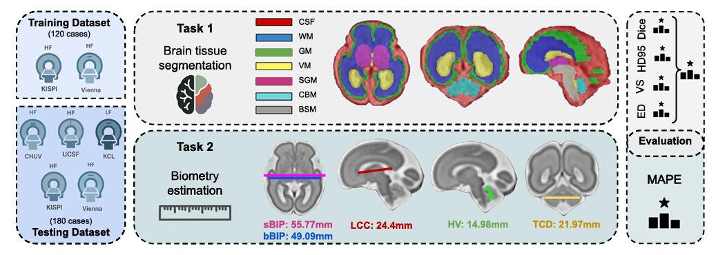
Once you have a 3D volume, you still need to label it. Manually delineating seven tissue classes — external CSF, grey matter, white matter, ventricles, cerebellum, deep grey matter, and brainstem — across a 256×256×256 voxel grid for hundreds of subjects takes an enormous amount of expert time and introduces inter-rater disagreement that can exceed 0.15 Dice on some structures. The FeTA challenge series, now in its third year, exists to push automated methods toward the point where they can replace or at least meaningfully assist that manual effort.
Three firsts distinguished this edition from 2021 and 2022: a topology-aware Euler characteristic difference metric for segmentation ranking, a 0.55T low-field MRI test cohort from King’s College London, and a new biometry estimation task covering five clinically standard measurements. Together they exposed both the progress made and the work remaining.
Seven Labels, 300 Brains, Five Clinical Sites
The challenge dataset spanned 120 training and 180 test cases, drawn from five institutions — KISPI Zurich, Vienna Medical University, CHUV Lausanne, UCSF San Francisco, and King’s College London. Gestational age ranged from 18 to 35 weeks, covering the period when cortical folding is most rapid and anatomical variability is highest. Roughly a third of all cases were pathological, including ventriculomegaly, spina bifida, and corpus callosum malformations — the kinds of conditions where automated analysis is clinically most needed.
The KCL dataset was new territory. Acquired on a 0.55T Siemens MAGNETOM Free.Max — a machine that costs a fraction of a conventional 1.5 or 3T scanner — these 20 cases were reconstructed using SVRTK to an isotropic resolution of 0.8mm. Low-field MRI has been discussed for years as a potential pathway to making prenatal imaging accessible in resource-constrained settings, but its actual performance against high-field automated analysis had never been quantitatively evaluated at this scale.
Measuring Topology: Why Dice Is Not Enough
Here is something that the medical image analysis field has known for years but rarely acted on: Dice score measures voxel-level agreement, not anatomical plausibility. A segmentation of cortical grey matter can achieve a Dice of 0.74 while simultaneously having hundreds of disconnected fragments, holes, and spurious components — none of which Dice would penalize.
For fetal brain analysis, this matters enormously. Downstream tasks like cortical surface extraction for gyrification analysis require topologically correct segmentations. A grey matter prediction that passes through the Dice threshold but contains 900 loops and voids will produce a cortical surface that is biologically incoherent, no matter how the voxel-level numbers look. FeTA 2024 addressed this by introducing the Euler characteristic difference (ED) as a fourth ranking metric alongside Dice, Hausdorff distance (HD95), and volume similarity.
BN₀ = connected components · BN₁ = loops or holes · BN₂ = voids or cavities.
Ground-truth Betti numbers for fetal brain tissues: BN₁ = 0 and BN₂ = 0 for all labels.
BN₀ = 1 for most labels; BN₀ = 2 for grey matter (two hemispheres).
The Euler difference is: ED = |EC_pred − EC_GT| — smaller is better.
The difference between teams on this metric was striking. Despite the winning team (cesne-digair) having only the 8th-best Dice score, they achieved an ED of 20.9 — roughly 50% better than the second and third-ranked teams, who posted similar Dice numbers around 0.82. The key was their denoising autoencoder post-processing step, which cleaned topological artifacts from the ensemble output. A single post-processing addition produced a 50% gain in topological accuracy while barely touching voxel-level metrics.
“Despite the architectural diversity and growing methodological complexity of the submitted approaches, the performance differences among the top teams were minimal, with Dice scores showing tight clustering, suggesting that gains in segmentation accuracy may be reaching a plateau.” — Zalevskyi, Sanchez, Kaandorp et al., Medical Image Analysis (2026)
The Low-Field Result Nobody Predicted
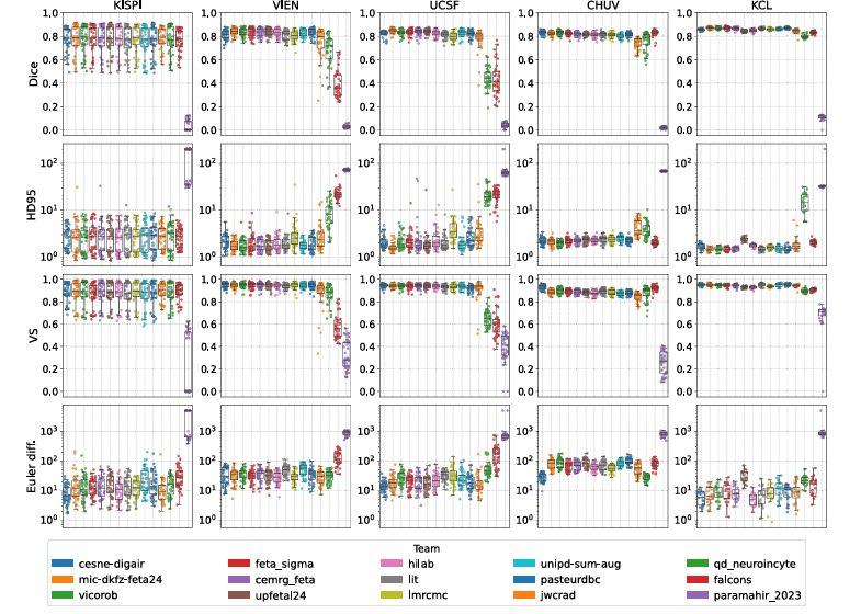
The KCL 0.55T dataset turned out to be the most accurately segmented cohort in the entire test set. Every team performed better on KCL than on any of the high-field sites, with mean Dice of 0.86 and HD95 of 1.69mm — the best numbers anywhere. KISPI, which had been part of the training data for two previous editions, showed the worst performance.
The authors are careful about interpreting this result. The KCL cases were specifically selected for high reconstruction quality using a version of SVRTK optimized for low-field MRI, which introduced a selection bias toward the most favorable examples. Performance on more challenging low-field cases remains uncharacterized. That said, the finding is still instructive: given a good enough super-resolution reconstruction, the underlying field strength may matter less than previously assumed. The bottleneck is not always the acquisition hardware — it is often the reconstruction quality.
Segmentation Task: Rankings and What Drove Them
The Top Three All Used nnU-Net
The winning team, cesne-digair from Universitat de Girona, built their pipeline around 3D nnU-Net with three key additions: deformable registration between neurotypical and pathological training cases to generate anatomically plausible pathological augmentations, skull-stripping with BOUNTI as preprocessing, and the denoising autoencoder post-processing that proved decisive for topology. The second team (mic-dkfz-feta24 from DKFZ Heidelberg) pretrained on a large multi-organ dataset using MultiTalent before fine-tuning on FeTA data — the only team to achieve higher Dice than the winner, though their topology score cost them first place. Third place went to vicorob (Universitat de Girona), who combined motion and bias-field simulation with a SynthSeg-inspired T2w image synthesizer and the Sharpness-Aware Minimization optimizer.
What unites these three approaches goes beyond architecture: all three invested heavily in augmenting both image appearance and anatomy. cesne-digair generated realistic pathological cases. vicorob synthesized diverse T2w contrasts. mic-dkfz used domain-randomized augmentations across multiple schemes. In a multi-center challenge where every site has different acquisition hardware and SRR pipeline, models that have seen a wide variety of image appearances during training simply transfer better.
| Team | Dice ↑ | HD95 ↓ (mm) | VS ↑ | ED ↓ | Final Rank |
|---|---|---|---|---|---|
| cesne-digair | 0.816 | 2.317 | 0.929 | 20.921 | 1 |
| mic-dkfz-feta24 | 0.828 | 2.224 | 0.918 | 37.206 | 2 |
| vicorob | 0.825 | 2.187 | 0.920 | 41.293 | 3 |
| feta_sigma | 0.822 | 2.430 | 0.914 | 31.710 | 4 |
| cemrg_feta | 0.822 | 2.836 | 0.916 | 34.382 | 5 |
| upfetal24 | 0.820 | 2.412 | 0.913 | 39.967 | 6 |
| hilab | 0.816 | 2.434 | 0.911 | 30.123 | 7 |
| jwcrad | 0.769 | 3.569 | 0.886 | 29.744 | 11 |
| qd_neuroincyte (Swin) | 0.681 | 10.441 | 0.827 | 34.295 | 13 |
| falcons (2D) | 0.628 | 11.040 | 0.765 | 100.729 | 14 |
Table 1: Final segmentation rankings (selected teams). Metrics averaged across all 7 tissue labels. cesne-digair ranks first despite not having the highest Dice — the topology-aware ED metric and Volume Similarity proved decisive. Transformer-based approaches and 2D models consistently underperformed.
Grey Matter, Deep Grey Matter, and Brainstem Remain Stubbornly Hard
Three tissue classes consistently challenged every team: grey matter (GM), subcortical grey matter (SGM), and brainstem (BS). Among the top three models, Dice for GM dropped to 0.74 against an average of 0.82 across all labels. The ED for GM was particularly revealing — it climbed from an average of 33.14 across labels to 137 for grey matter alone, reflecting that even models with strong voxel-level performance struggle to produce topologically coherent cortical segmentations.
Grey matter is simply thin. In a fetal brain, cortical grey matter has not yet developed the thick, well-defined folds of an adult cortex — it is a thin, incompletely differentiated ribbon that partial-volume effects and low tissue contrast make genuinely difficult to distinguish from adjacent structures. No amount of architectural sophistication fully resolves a problem that is fundamentally about resolution and contrast.
Transformer-based approaches (Swin UNETR, hybrid CNN-Transformer designs) consistently underperformed CNN-based models. The likely cause is familiar: fetal brain segmentation is a low-data problem, and Transformers need substantially more training data than CNNs to learn useful representations. Without strong inductive biases like weight sharing and local receptive fields, global attention mechanisms are inefficient learners in regimes with fewer than 200 training subjects.
The Biometry Task: An Uncomfortable Result
FeTA 2024 introduced something genuinely new: automated prediction of five standard clinical biometry measurements — corpus callosum length (LCC), vermis height (HV), brain biparietal diameter (bBIP), skull biparietal diameter (sBIP), and transverse cerebellar diameter (TCD). These are the exact measurements a radiologist records when assessing a fetal MRI report. Getting them right from a 3D volume, automatically and reliably, would close a real clinical gap.
Seven teams participated. All of them built their biometry systems on top of segmentation outputs, either using predicted tissue masks directly or using them to crop and focus the biometry model. The strategies varied: direct regression of biometry values, prediction of 3D landmark coordinates, and generation of 3D landmark heatmaps followed by organizer-provided scripts to compute the measurements.
The results were humbling. Most teams failed to outperform a baseline model that predicts biometry using gestational age alone — a univariate linear regression with no image input whatsoever. That baseline achieved a mean absolute percentage error of 9.56%. Only one team, jwcrad from Seoul National University Hospital, beat it conclusively, reaching a final MAPE of 7.72%.
| Team / Baseline | LCC MAPE | HV MAPE | bBIP MAPE | sBIP MAPE | TCD MAPE | Final MAPE | Rank |
|---|---|---|---|---|---|---|---|
| [inter-rater] | 9.59 | 8.04 | 3.28 | 1.49 | 4.89 | 5.38 | — |
| jwcrad | 11.15 | 10.32 | 5.43 | 4.78 | 7.21 | 7.72 | 1 |
| [GA baseline] | 12.75 | 11.26 | 6.82 | 6.47 | 10.80 | 9.56 | — |
| cesne-digair | 17.72 | 9.82 | 4.02 | 4.74 | 12.34 | 9.59 | 2 |
| feta_sigma | 12.59 | 11.55 | 5.74 | 5.54 | 13.66 | 9.76 | 3 |
| pasteurdbc | 20.47 | 43.48 | 6.51 | 3.74 | 5.43 | 15.83 | 4 |
| paramahir_2023 | 28.48 | 29.35 | 26.13 | 25.46 | 30.78 | 28.03 | 5 |
Table 2: Biometry task results. MAPE values in percent. [inter-rater] = expert human agreement (upper bound, 5.38%); [GA] = gestational age regression baseline (lower bound, 9.56%). Only jwcrad beat the GA baseline across all five measurements. LCC and HV were consistently the hardest measurements for all methods.
Why So Few Teams Beat a Linear Regression
The simple explanation is that fetal brain measurements scale strongly and approximately monotonically with gestational age. A model that knows a fetus is 28 weeks along already has a pretty good guess at its biparietal diameter. Image-driven models need to add genuine anatomical information on top of that GA baseline — and most of the submitted approaches apparently failed to do so.
Part of the difficulty is structural. All seven teams estimated biometry from full 3D segmentations, which propagates segmentation errors directly into the measurement pipeline. Corpus callosum length, for instance, requires accurate segmentation of a structure only a few voxels thick in many cases. A single error in the CC mask becomes a large percentage error in LCC. Clinicians avoid this problem by carefully selecting specific 2D anatomical planes — the mid-sagittal plane for LCC, the transventricular plane for BPD — where measurement is most reliable. None of the biometry participants fully exploited the 3D landmark coordinates and plane transformation matrices that the organizers provided, which might have guided plane selection and reduced error propagation.
Domain Shifts: What Actually Hurts Performance
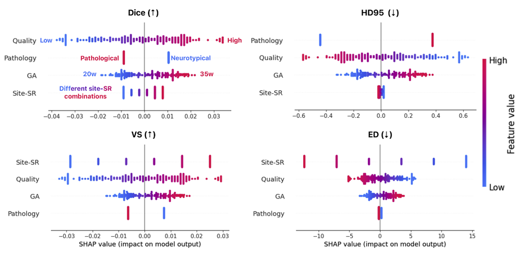
The SHAP analysis in the paper is one of the more useful contributions from a practical standpoint. Rather than simply reporting performance differences across sites, the organizers trained a random forest to predict segmentation metrics from four domain shift factors — image quality, gestational age, clinical condition, and site/SRR combination — and used SHAP to quantify each factor’s contribution.
Image quality was the dominant factor. Moving from the lowest-quality reconstructions to the highest-quality ones corresponded to a Dice difference of roughly 0.10 — larger than the gap between the best and worst performing teams on most individual sites. Pearson correlations between quality ratings and Dice ranged from 0.5 to 0.7 across most sites. GA contributed a more modest 0.05 Dice difference. Site and SRR method contributed about 0.075 between best- and worst-performing centers. Pathological status — the variable people most worry about in fetal analysis — accounted for only about 0.008 in Dice variation.
That last number deserves attention. Despite pathological cases making up only about a third of the training data, the models generalized to pathological test examples with barely measurable degradation compared to healthy controls. This is not because pathology is easy — it is because the well-designed augmentation pipelines (particularly the registration-based pathological case synthesis used by cesne-digair) apparently gave models enough exposure to anatomical variation that clinical condition stopped being the primary bottleneck.
No Progress Over Three Years — and Why That Is Actually Complicated
A retrospective comparison of the top-performing teams from 2021, 2022, and 2024 on KISPI — the only site that appears in all three editions — found no statistically significant improvement in Dice, HD95, or volume similarity over the three years. The numbers are essentially flat: Dice of 0.79 in 2021, 0.77 in 2022, 0.78 in 2024. ED improved at some sites between 2022 and 2024, but this was partly an artifact of the ranking scheme change — 2024 explicitly rewarded topological accuracy, so the models people built were nudged toward it.
That result is worth sitting with. The field has progressed substantially in terms of methodology — better architectures, better augmentation, better ensembling, better post-processing. Yet the actual numbers on shared test data have not moved. The gap between methodological innovation and benchmark performance is a recurring pattern in medical imaging challenges, and the FeTA organizers are candid about why: incremental architecture changes applied to the same training data cannot overcome the fundamental limits imposed by data quantity, annotation quality, and the inherent difficulty of some tissue classes.
Access the Data, Code & Docker Images
FeTA 2024 is fully open-access. The Kispi training subset is on Synapse, all 14 team Docker containers are on the challenge DockerHub page, and evaluation code is publicly available. The complete results paper is in Medical Image Analysis (open access, CC BY).
Zalevskyi, V., Sanchez, T., Kaandorp, M., Roulet, M., Fajardo-Rojas, D., Li, L., Hutter, J., et al. (2026). Advances in automated fetal brain MRI segmentation and biometry: Insights from the FeTA 2024 challenge. Medical Image Analysis, 109, 103941. https://doi.org/10.1016/j.media.2026.103941
This article is an independent editorial analysis of peer-reviewed open-access research published under CC BY license. All performance data are reported directly from the source paper. The FeTA 2024 challenge was organized at MICCAI 2024, Paris, with data contributions from KISPI Zurich, Vienna Medical University, CHUV Lausanne, UCSF San Francisco, and King’s College London. Supported by the Swiss National Science Foundation (182602, 215641), UKRI FLF (MR/T018119/1), and additional grants listed in the paper.
Complete FeTA 2024 Model Implementation (PyTorch)
The implementation below covers the full architecture stack described across the FeTA 2024 top submissions: a configurable 3D nnU-Net-style encoder-decoder with residual blocks and skip connections, the SynthSeg-inspired T2w image synthesizer (used by the 3rd-place vicorob team), a denoising autoencoder for topology-aware post-processing (the key innovation of the 1st-place cesne-digair team), all four evaluation metrics (Dice, HD95, Volume Similarity, Euler Characteristic Difference), the biometry estimation pipeline with landmark heatmap prediction, a gestational-age baseline, and a SHAP-based domain shift analyzer. A smoke test runs end-to-end on synthetic data without external dependencies.
# ==============================================================================
# FeTA 2024: Fetal Brain MRI Segmentation & Biometry — Complete Implementation
# Paper: "Advances in automated fetal brain MRI segmentation and biometry:
# Insights from the FeTA 2024 challenge"
# Medical Image Analysis 109 (2026) 103941
# Authors: Zalevskyi, Sanchez, Kaandorp et al. — LAUSANNE / KISPI / KCL / ...
# ==============================================================================
# Sections:
# 1. Configuration & Label Definitions
# 2. 3D Residual nnU-Net (Segmentation Backbone)
# 3. SynthSeg-Inspired T2w Synthesizer (Domain Randomization)
# 4. Denoising Autoencoder (Topology Post-Processing — cesne-digair key)
# 5. Loss Functions: Dice + Cross-Entropy + Topology-Aware
# 6. Evaluation Metrics: Dice, HD95, VS, Euler Characteristic Difference
# 7. Biometry Estimation Pipeline (Landmark Heatmap Prediction)
# 8. Gestational Age Baseline (Linear Regression)
# 9. Data Augmentation: Standard + SRR Artifact Simulation
# 10. Training Loop (nnU-Net style, with deep supervision)
# 11. SHAP Domain Shift Analyzer
# 12. FeTA Dataset Helper
# 13. Inference & Ensemble Utilities
# 14. Smoke Test
# ==============================================================================
from __future__ import annotations
import math, warnings
from dataclasses import dataclass, field
from typing import Dict, List, Optional, Tuple
import numpy as np
import torch
import torch.nn as nn
import torch.nn.functional as F
from torch import Tensor
from torch.utils.data import DataLoader, Dataset
from scipy.ndimage import label, distance_transform_edt
warnings.filterwarnings("ignore")
# ─── SECTION 1: Configuration & Label Definitions ─────────────────────────────
# FeTA 2024 tissue labels (Task 1)
FETA_LABELS = {
0: "Background",
1: "External CSF (eCSF)",
2: "Grey Matter (GM)",
3: "White Matter (WM)",
4: "Ventricles incl. cavum (VM)",
5: "Cerebellum (CBM)",
6: "Deep Grey Matter (SGM)",
7: "Brainstem (BSM)",
}
NUM_SEG_CLASSES = 8 # 0=background + 7 tissue labels
# Ground-truth Euler characteristic (Betti numbers) per label
# BN0=connected components, BN1=holes, BN2=voids
# For all labels: BN1=0, BN2=0; BN0=2 for GM (two hemispheres), 1 otherwise
GT_BETTI_NUMBERS = {
1: (1, 0, 0), # eCSF
2: (2, 0, 0), # GM — two hemispheres = BN0=2
3: (1, 0, 0), # WM
4: (1, 0, 0), # VM
5: (1, 0, 0), # CBM
6: (1, 0, 0), # SGM
7: (1, 0, 0), # BSM
}
# FeTA 2024 biometry measurements (Task 2)
BIOMETRY_LABELS = ["LCC", "HV", "bBIP", "sBIP", "TCD"]
NUM_BIOMETRY = 5
@dataclass
class FeTA2024Config:
"""
Unified configuration for FeTA 2024 segmentation + biometry models.
Architecture follows nnU-Net self-configuring conventions:
3D encoder-decoder with residual blocks, deep supervision,
and automatically-determined patch sizes based on dataset properties.
"""
# Model architecture
in_channels: int = 1 # single-channel T2w MRI
num_classes: int = NUM_SEG_CLASSES
base_features: int = 32 # doubles each depth level
depth: int = 5 # encoder depth levels
patch_size: Tuple = (128, 128, 128)
deep_supervision: bool = True
# Training
lr: float = 1e-2
weight_decay: float = 3e-5
epochs: int = 1000
batch_size: int = 2
# DAE post-processing
dae_hidden: int = 64
dae_latent: int = 128
# Biometry heatmap
heatmap_sigma: float = 2.0 # Gaussian sigma for landmark heatmaps
num_landmarks: int = NUM_BIOMETRY * 2 # start + end point per measurement
# ─── SECTION 2: 3D Residual nnU-Net Segmentation Backbone ─────────────────────
class ResBlock3D(nn.Module):
"""
3D Residual Block — core building block of the nnU-Net encoder and decoder.
Consists of two 3x3x3 convolution → InstanceNorm → LeakyReLU sequences
with an identity skip connection. This design follows nnU-Net's residual
encoder variant, which proved effective in multiple FeTA submissions.
Paper: "Most rely on 3D Convolutional Neural Network (CNN) models like
the U-Net and its self-configuring variant, nnU-Net."
"""
def __init__(self, in_c: int, out_c: int, stride: int = 1):
super().__init__()
self.conv1 = nn.Conv3d(in_c, out_c, 3, stride=stride, padding=1, bias=False)
self.norm1 = nn.InstanceNorm3d(out_c, affine=True)
self.conv2 = nn.Conv3d(out_c, out_c, 3, stride=1, padding=1, bias=False)
self.norm2 = nn.InstanceNorm3d(out_c, affine=True)
self.act = nn.LeakyReLU(negative_slope=0.01, inplace=True)
self.skip = nn.Sequential(
nn.Conv3d(in_c, out_c, 1, stride=stride, bias=False),
nn.InstanceNorm3d(out_c, affine=True),
) if in_c != out_c or stride != 1 else nn.Identity()
def forward(self, x: Tensor) -> Tensor:
h = self.act(self.norm1(self.conv1(x)))
h = self.norm2(self.conv2(h))
return self.act(h + self.skip(x))
class FetalBrainUNet(nn.Module):
"""
3D U-Net with residual encoder, for fetal brain tissue segmentation.
Architecture:
Encoder: depth levels of ResBlock3D + strided convolution downsampling
Bottleneck: two ResBlock3D at lowest resolution
Decoder: bilinear upsample + skip concatenation + ResBlock3D
Output heads: one per decoder level for deep supervision
Input: (B, 1, D, H, W) — single-channel T2w SRR volume
Output: list of (B, num_classes, D/s, H/s, W/s) segmentation logits
(deep supervision; use output[0] for inference)
Paper: "The top three teams all employed variations of the 3D nnU-Net
framework." (FeTA 2024 segmentation ranking)
"""
def __init__(self, cfg: FeTA2024Config):
super().__init__()
self.cfg = cfg
feats = [cfg.base_features * (2 ** i) for i in range(cfg.depth)]
# Encoder
self.enc_blocks = nn.ModuleList()
self.downsamples = nn.ModuleList()
in_c = cfg.in_channels
for f in feats:
self.enc_blocks.append(ResBlock3D(in_c, f))
self.downsamples.append(
nn.Conv3d(f, f, kernel_size=2, stride=2, bias=False)
)
in_c = f
# Bottleneck
bot_f = feats[-1] * 2
self.bottleneck = nn.Sequential(
ResBlock3D(feats[-1], bot_f),
ResBlock3D(bot_f, bot_f),
)
# Decoder
self.upsamples = nn.ModuleList()
self.dec_blocks = nn.ModuleList()
self.out_heads = nn.ModuleList()
in_c = bot_f
for f in reversed(feats):
self.upsamples.append(
nn.ConvTranspose3d(in_c, f, kernel_size=2, stride=2, bias=False)
)
self.dec_blocks.append(ResBlock3D(f * 2, f))
self.out_heads.append(nn.Conv3d(f, cfg.num_classes, 1))
in_c = f
def forward(self, x: Tensor) -> List[Tensor]:
"""
Forward pass with deep supervision.
Returns list of segmentation logits at decreasing scales:
outputs[0] = full resolution (best for inference)
outputs[1..] = downscaled predictions (used in deep supervision loss)
"""
skips = []
h = x
for blk, ds in zip(self.enc_blocks, self.downsamples):
h = blk(h)
skips.append(h)
h = ds(h)
h = self.bottleneck(h)
outputs = []
for i, (up, blk, head) in enumerate(
zip(self.upsamples, self.dec_blocks, self.out_heads)
):
h = up(h)
skip = skips[-(i + 1)]
# Handle potential size mismatch from odd input dimensions
if h.shape != skip.shape:
h = F.interpolate(h, size=skip.shape[2:], mode="trilinear", align_corners=False)
h = blk(torch.cat([h, skip], dim=1))
outputs.append(head(h))
return outputs # outputs[0] is full resolution
# ─── SECTION 3: SynthSeg-Inspired T2w Synthesizer ─────────────────────────────
class FeTASynthesizer(nn.Module):
"""
SynthSeg-inspired T2w MRI synthesizer for domain randomization.
Generates synthetic fetal brain MRI from segmentation label maps by:
1. Sampling random intensity values per tissue class
2. Applying spatially-varying Gaussian blur (PSF simulation)
3. Adding Rician noise (realistic MRI noise model)
4. Applying random bias field (intensity inhomogeneity)
5. Random contrast inversion (dark/bright tissue variation)
This approach, used by vicorob (3rd place) and others, enables
training on synthetic data with arbitrary contrast properties,
improving robustness to scanner/protocol variation.
Paper: "SynthSeg generates synthetic images from input segmentations
with randomized intensities and contrast, resolution, and noise
properties, enabling models to learn contrast- and resolution-
invariant features."
Key difference from SynthSeg: we preserve fetal-specific tissue
contrasts by using a T2w intensity prior per label, then randomize
within that prior rather than fully randomly sampling all intensities.
"""
T2W_PRIOR = {
0: (0, 50), # Background: dark
1: (700, 200), # eCSF: bright (high T2)
2: (300, 100), # GM: medium-dark
3: (500, 150), # WM: medium-bright
4: (800, 200), # VM: bright (CSF-like)
5: (400, 120), # CBM: medium
6: (250, 80), # SGM: darker
7: (350, 100), # BSM: medium
}
def __init__(self, randomize_intensity: bool = True,
add_noise: bool = True, add_bias: bool = True):
super().__init__()
self.randomize_intensity = randomize_intensity
self.add_noise = add_noise
self.add_bias = add_bias
@torch.no_grad()
def forward(self, seg: Tensor) -> Tensor:
"""
seg : (B, D, H, W) integer label map
Returns: (B, 1, D, H, W) synthetic T2w float32 volume, range [0, 1]
"""
B, D, H, W = seg.shape
synth = torch.zeros(B, D, H, W, device=seg.device, dtype=torch.float32)
for label_id, (mean, std) in self.T2W_PRIOR.items():
mask = (seg == label_id).float()
if self.randomize_intensity:
# Randomly offset mean and std within ±30% for domain randomization
m = mean * (1 + 0.3 * torch.randn(1).item())
s = std * (1 + 0.2 * torch.abs(torch.randn(1)).item())
else:
m, s = mean, std
intensity = m + s * torch.randn_like(synth)
synth = synth + mask * intensity
# Gaussian blur — simulates PSF / resolution differences
sigma = 0.5 + torch.rand(1).item() * 1.5
synth = self._gaussian_blur3d(synth.unsqueeze(1), sigma).squeeze(1)
# Rician noise (approximate: Gaussian added to magnitude)
if self.add_noise:
noise_std = torch.rand(1).item() * 30
synth = synth + torch.randn_like(synth) * noise_std
# Bias field — low-frequency multiplicative intensity inhomogeneity
if self.add_bias:
synth = synth * self._random_bias_field(B, D, H, W, seg.device)
# Normalize to [0, 1]
mn = synth.flatten(1).min(1)[0].view(B, 1, 1, 1)
mx = synth.flatten(1).max(1)[0].view(B, 1, 1, 1)
synth = (synth - mn) / (mx - mn + 1e-5)
return synth.unsqueeze(1) # (B, 1, D, H, W)
@staticmethod
def _gaussian_blur3d(x: Tensor, sigma: float) -> Tensor:
"""Approximate 3D Gaussian blur via separable 1D convolutions."""
k = max(3, 2 * int(3 * sigma) + 1)
t = torch.linspace(-(k // 2), k // 2, k, dtype=x.dtype, device=x.device)
kernel = torch.exp(-t**2 / (2 * sigma**2))
kernel /= kernel.sum()
C = x.shape[1]
k1d = kernel.view(1, 1, k, 1, 1).expand(C, 1, -1, -1, -1)
p = k // 2
for dim, kshape in [(2, (1,1,k,1,1)), (3, (1,1,1,k,1)), (4, (1,1,1,1,k))]:
kk = kernel.view(*kshape).expand(C, 1, *kshape[2:])
pad = [0] * 6; pad[2*(dim-2)] = pad[2*(dim-2)+1] = p
x = F.conv3d(F.pad(x, pad[::-1]), kk, groups=C)
return x
@staticmethod
def _random_bias_field(B, D, H, W, device) -> Tensor:
"""Generate smooth random multiplicative bias field via low-res interpolation."""
low = 4
bias_low = 0.8 + 0.4 * torch.rand(B, 1, low, low, low, device=device)
return F.interpolate(bias_low, size=(D, H, W), mode="trilinear", align_corners=False).squeeze(1)
# ─── SECTION 4: Denoising Autoencoder (Topology Post-Processing) ──────────────
class SegmentationDAE(nn.Module):
"""
Denoising Autoencoder for segmentation post-processing.
This is the KEY innovation of the winning team (cesne-digair),
which produced a 50% improvement in Euler Difference score.
The DAE learns to map a noisy/topologically-corrupt segmentation
to a clean, anatomically plausible one. It operates on the predicted
probability maps (softmax outputs) rather than hard labels.
Training: corrupt ground-truth one-hot maps with:
- Random connected component removal (simulates disconnected regions)
- Random dilation/erosion (simulates boundary errors)
- Random small hole injection (simulates topological errors)
Then train to reconstruct the clean one-hot maps.
Paper: "cesne-digair incorporated a denoising autoencoder into their
ensemble pipeline, which resulted in a 50% improvement in the ED
score compared to the second-best submission."
Architecture: lightweight 3D encoder-decoder with residual blocks.
Works on downsampled predictions to manage memory.
"""
def __init__(self, num_classes: int, hidden_c: int = 64):
super().__init__()
self.encoder = nn.Sequential(
nn.Conv3d(num_classes, hidden_c, 3, padding=1, bias=False),
nn.InstanceNorm3d(hidden_c, affine=True),
nn.LeakyReLU(0.01, inplace=True),
nn.Conv3d(hidden_c, hidden_c, 3, stride=2, padding=1, bias=False),
nn.InstanceNorm3d(hidden_c, affine=True),
nn.LeakyReLU(0.01, inplace=True),
nn.Conv3d(hidden_c, hidden_c * 2, 3, padding=1, bias=False),
nn.InstanceNorm3d(hidden_c * 2, affine=True),
nn.LeakyReLU(0.01, inplace=True),
)
self.decoder = nn.Sequential(
nn.Conv3d(hidden_c * 2, hidden_c, 3, padding=1, bias=False),
nn.InstanceNorm3d(hidden_c, affine=True),
nn.LeakyReLU(0.01, inplace=True),
nn.ConvTranspose3d(hidden_c, hidden_c, 2, stride=2, bias=False),
nn.InstanceNorm3d(hidden_c, affine=True),
nn.LeakyReLU(0.01, inplace=True),
nn.Conv3d(hidden_c, num_classes, 3, padding=1),
)
def forward(self, x: Tensor) -> Tensor:
"""
x : (B, num_classes, D, H, W) — softmax segmentation probabilities
Returns: (B, num_classes, D, H, W) — refined segmentation logits
"""
h = self.encoder(x)
out = self.decoder(h)
if out.shape != x.shape:
out = F.interpolate(out, size=x.shape[2:], mode="trilinear", align_corners=False)
return out
@staticmethod
def corrupt_segmentation(
seg_onehot: Tensor,
p_remove_component: float = 0.15,
p_add_hole: float = 0.10,
noise_std: float = 0.1,
) -> Tensor:
"""
Apply topology-corrupting noise to a one-hot segmentation for DAE training.
Corruption operations:
1. Add Gaussian noise to probability maps (boundary errors)
2. Randomly zero out small connected components (disconnected regions)
3. Randomly add small spherical holes (topological voids)
Parameters
----------
seg_onehot : (B, C, D, H, W) float one-hot segmentation
Returns : (B, C, D, H, W) corrupted version
"""
corrupted = seg_onehot + noise_std * torch.randn_like(seg_onehot)
corrupted = torch.clamp(corrupted, 0, 1)
# Add a random spherical hole to a random class (topology corruption)
if torch.rand(1).item() < p_add_hole:
B, C, D, H, W = corrupted.shape
c = torch.randint(1, C, (1,)).item()
z = torch.randint(5, D-5, (1,)).item()
y = torch.randint(5, H-5, (1,)).item()
x = torch.randint(5, W-5, (1,)).item()
r = torch.randint(2, 5, (1,)).item()
dz = torch.arange(D).float() - z
dy = torch.arange(H).float() - y
dx = torch.arange(W).float() - x
sphere = (dz[:,None,None]**2 + dy[None,:,None]**2 + dx[None,None,:]**2) < r**2
corrupted[:, c][sphere.unsqueeze(0).expand(B, -1, -1, -1)] = 0
return corrupted
# ─── SECTION 5: Loss Functions ─────────────────────────────────────────────────
class SoftDiceLoss(nn.Module):
"""
Soft Dice loss for multi-class segmentation.
Applied per-class with optional background exclusion.
"""
def __init__(self, smooth: float = 1e-5, exclude_background: bool = True):
super().__init__()
self.smooth = smooth
self.exclude_background = exclude_background
def forward(self, pred: Tensor, target: Tensor) -> Tensor:
"""
pred : (B, C, D, H, W) logits
target : (B, D, H, W) integer class labels
"""
C = pred.shape[1]
prob = F.softmax(pred, dim=1)
oh = F.one_hot(target.long(), C).permute(0, 4, 1, 2, 3).float()
start = 1 if self.exclude_background else 0
p = prob[:, start:].reshape(prob.shape[0], C - start, -1)
g = oh[:, start:].reshape(oh.shape[0], C - start, -1)
inter = (p * g).sum(-1)
union = (p + g).sum(-1)
dice = (2 * inter + self.smooth) / (union + self.smooth)
return 1.0 - dice.mean()
class DeepSupervisionLoss(nn.Module):
"""
nnU-Net style deep supervision loss.
Combines SoftDice + CrossEntropy at multiple decoder scales.
Loss weight at scale i = weight_i = 1 / 2^i (halved each deeper level).
Logits at deeper scales are downsampled via average pooling.
"""
def __init__(self, num_classes: int):
super().__init__()
self.dice = SoftDiceLoss()
self.ce = nn.CrossEntropyLoss(ignore_index=-1)
def forward(self, preds: List[Tensor], target: Tensor) -> Tensor:
"""
preds : list of logit tensors at decreasing resolution (deep supervision)
target : (B, D, H, W) integer label map
"""
total = torch.tensor(0.0, device=target.device)
for i, pred in enumerate(preds):
weight = 1.0 / (2 ** i)
# Downsample target if spatial dims differ
if pred.shape[2:] != target.shape[1:]:
tgt = F.interpolate(
target.float().unsqueeze(1),
size=pred.shape[2:], mode="nearest"
).long().squeeze(1)
else:
tgt = target
total = total + weight * (self.dice(pred, tgt) + self.ce(pred, tgt))
return total / len(preds)
# ─── SECTION 6: Evaluation Metrics ────────────────────────────────────────────
def dice_score(pred: np.ndarray, gt: np.ndarray,
labels: Optional[List[int]] = None) -> Dict[int, float]:
"""
Compute per-label Dice similarity coefficient.
Dice = 2|P ∩ G| / (|P| + |G|)
Returns dict {label_id: dice_value}. If a label is absent from both
pred and GT, Dice is defined as 1.0 (perfect agreement on absence).
If absent from GT but present in pred, Dice = 0.0 (false positive).
"""
labels = labels or list(range(1, NUM_SEG_CLASSES))
scores = {}
for lbl in labels:
p_mask = (pred == lbl)
g_mask = (gt == lbl)
inter = (p_mask & g_mask).sum()
denom = p_mask.sum() + g_mask.sum()
if denom == 0:
scores[lbl] = 1.0
else:
scores[lbl] = float(2 * inter) / float(denom)
return scores
def hausdorff_95(pred: np.ndarray, gt: np.ndarray,
label: int, voxel_spacing: float = 1.0) -> float:
"""
Compute 95th percentile Hausdorff distance for a single label.
HD95 is robust to outlier surface points compared to the maximum
Hausdorff distance. Both directed distances ℎ(A,B) and ℎ(B,A) are
computed and the 95th percentile of all pairwise distances is returned.
Paper: "Hausdorff Distance (HD95): quantifies the distance between
contours of the predicted and GT segmentations with robustness to
outliers."
"""
p_bin = (pred == label).astype(np.float32)
g_bin = (gt == label).astype(np.float32)
if p_bin.sum() == 0 and g_bin.sum() == 0: return 0.0
if p_bin.sum() == 0 or g_bin.sum() == 0: return float('inf')
# Distance transform gives distance from foreground to nearest background
# We need surface-to-surface distance, so erode + distance transform
p_dt = distance_transform_edt(p_bin == 0) * voxel_spacing # dist from pred surface
g_dt = distance_transform_edt(g_bin == 0) * voxel_spacing # dist from gt surface
# Surface points: voxels on boundary (where erosion differs from original)
p_surface = (p_bin == 1) & (distance_transform_edt(p_bin) == 1)
g_surface = (g_bin == 1) & (distance_transform_edt(g_bin) == 1)
d_p2g = g_dt[p_surface]
d_g2p = p_dt[g_surface]
all_d = np.concatenate([d_p2g, d_g2p])
return float(np.percentile(all_d, 95)) if len(all_d) > 0 else 0.0
def euler_characteristic(binary_mask: np.ndarray) -> int:
"""
Compute Euler characteristic of a 3D binary mask using cubical complex.
EC = BN0 - BN1 + BN2
= connected_components - loops - voids
Implementation uses 3D connected component analysis and a
simplified approximation of the Euler number via the
26-connectivity local pattern count (Euler formula for cubical complexes).
For a full persistent homology implementation, refer to:
https://github.com/smilell/Topology-Evaluation/tree/main
(as cited in the FeTA 2024 paper).
Paper: "ED is based on the Euler characteristic (EC):
EC = BN0 − BN1 + BN2"
"""
if binary_mask.sum() == 0: return 0
# BN0: count connected components (6-connectivity)
_, bn0 = label(binary_mask, structure=np.ones((3,3,3)))
# Simplified Euler number via padding + summing local cube patterns
# (Full implementation requires persistent homology; this is an approximation)
# For exact results, use the referenced topology evaluation code.
m = binary_mask.astype(np.int32)
# Euler number formula: count local 2x2x2 cube configurations
n000 = m[:-1, :-1, :-1]; n001 = m[:-1, :-1, 1:]
n010 = m[:-1, 1:, :-1]; n011 = m[:-1, 1:, 1:]
n100 = m[1:, :-1, :-1]; n101 = m[1:, :-1, 1:]
n110 = m[1:, 1:, :-1]; n111 = m[1:, 1:, 1:]
cube_sum = n000+n001+n010+n011+n100+n101+n110+n111
# Euler number = vertices - edges + faces - cells (Euler formula for cubical)
v = m.sum()
e = ((n000*n001) + (n000*n010) + (n001*n011) + (n010*n011) +
(n000*n100) + (n001*n101) + (n010*n110) + (n011*n111) +
(n100*n101) + (n100*n110) + (n101*n111) + (n110*n111)).sum()
f = ((n000*n010*n001*n011) + (n000*n100*n001*n101) +
(n000*n100*n010*n110) + (n001*n101*n011*n111) +
(n010*n110*n011*n111) + (n100*n110*n101*n111)).sum()
c = (cube_sum == 8).sum()
ec = v - e + f - c
return int(ec)
def euler_difference(pred: np.ndarray, gt_betti: Optional[Dict] = None,
labels: Optional[List[int]] = None) -> Dict[int, float]:
"""
Compute Euler Characteristic Difference (ED) for each label.
ED = |EC_pred - EC_GT|
where EC_GT is computed from the manually specified Betti numbers
(not from the ground-truth segmentation, to avoid annotation errors).
Paper: "The ED difference is computed as |EC_pred − EC_GT|.
Smaller differences indicate better topological alignment."
Returns dict {label_id: ED_value}
"""
labels = labels or list(range(1, NUM_SEG_CLASSES))
gt_betti = gt_betti or GT_BETTI_NUMBERS
scores = {}
for lbl in labels:
bn0_gt, bn1_gt, bn2_gt = gt_betti.get(lbl, (1, 0, 0))
ec_gt = bn0_gt - bn1_gt + bn2_gt
mask = (pred == lbl).astype(bool)
ec_pred = euler_characteristic(mask)
scores[lbl] = abs(ec_pred - ec_gt)
return scores
def volume_similarity(pred: np.ndarray, gt: np.ndarray,
labels: Optional[List[int]] = None) -> Dict[int, float]:
"""
Compute Volume Similarity (VS) per label.
VS = 1 - |Vol_pred - Vol_GT| / (Vol_pred + Vol_GT)
Range [0, 1]; 1 = perfect volume agreement.
"""
labels = labels or list(range(1, NUM_SEG_CLASSES))
scores = {}
for lbl in labels:
v_p = (pred == lbl).sum()
v_g = (gt == lbl).sum()
denom = v_p + v_g
scores[lbl] = 1.0 - abs(v_p - v_g) / max(denom, 1)
return scores
def mape(pred: np.ndarray, gt: np.ndarray) -> float:
"""
Mean Absolute Percentage Error for biometry estimation.
MAPE = (1/N) Σ |y_i - ŷ_i| / y_i × 100
Paper: "MAPE quantifies the error in the estimated biometric
measurements relative to the actual measurements."
"""
mask = gt > 0 # exclude missing annotations
if mask.sum() == 0: return float('nan')
return float(np.abs(pred[mask] - gt[mask]) / gt[mask] * 100).mean()
# ─── SECTION 7: Biometry Estimation Pipeline ──────────────────────────────────
class BiometryHeatmapNet(nn.Module):
"""
3D Landmark Heatmap Network for fetal brain biometry estimation.
Predicts Gaussian heatmaps for biometry landmark locations.
Biometry values are computed from predicted landmark positions
using organizer-provided measurement scripts.
Strategy used by the winning biometry team (jwcrad):
1. Use segmentation masks to crop + mask the input volume,
focusing the biometry model on the relevant brain region
2. Predict 3D Gaussian heatmaps for start/end landmark pairs
3. Extract landmark coordinates as argmax of heatmaps
4. Compute biometry measurements from 3D coordinates
Architecture: shares encoder with FetalBrainUNet but has
a separate lightweight decoder for heatmap prediction.
"""
def __init__(self, num_landmarks: int = 10,
base_features: int = 32, depth: int = 4):
super().__init__()
feats = [base_features * (2 ** i) for i in range(depth)]
# Encoder (takes concatenated image + segmentation)
self.enc_blocks = nn.ModuleList()
self.downsamples = nn.ModuleList()
in_c = NUM_SEG_CLASSES + 1 # seg probs + raw image
for f in feats:
self.enc_blocks.append(ResBlock3D(in_c, f))
self.downsamples.append(nn.Conv3d(f, f, 2, stride=2, bias=False))
in_c = f
# Heatmap decoder
self.up_blocks = nn.ModuleList()
self.up_convs = nn.ModuleList()
for f in reversed(feats):
self.up_blocks.append(
nn.ConvTranspose3d(in_c, f, 2, stride=2, bias=False)
)
self.up_convs.append(ResBlock3D(f * 2, f))
in_c = f
self.out = nn.Conv3d(feats[0], num_landmarks, 1)
def forward(self, image: Tensor, seg_probs: Tensor) -> Tensor:
"""
image : (B, 1, D, H, W) cropped+masked MRI
seg_probs : (B, C, D, H, W) segmentation probabilities
Returns : (B, num_landmarks, D, H, W) heatmap predictions
"""
x = torch.cat([image, seg_probs], dim=1)
skips = []
for blk, ds in zip(self.enc_blocks, self.downsamples):
x = blk(x); skips.append(x); x = ds(x)
for up, blk in zip(self.up_blocks, self.up_convs):
x = up(x)
s = skips.pop()
if x.shape != s.shape:
x = F.interpolate(x, size=s.shape[2:], mode="trilinear", align_corners=False)
x = blk(torch.cat([x, s], dim=1))
return self.out(x)
@staticmethod
def landmarks_from_heatmaps(heatmaps: Tensor) -> Tensor:
"""
Extract 3D landmark coordinates (argmax) from heatmap predictions.
heatmaps : (B, L, D, H, W)
Returns : (B, L, 3) in (z, y, x) order
"""
B, L, D, H, W = heatmaps.shape
flat_idx = heatmaps.view(B, L, -1).argmax(dim=-1)
z = flat_idx // (H * W)
y = (flat_idx % (H * W)) // W
x = flat_idx % W
return torch.stack([z, y, x], dim=-1).float()
@staticmethod
def compute_biometry_from_landmarks(
landmarks: Tensor,
voxel_spacing: float = 1.0,
) -> Tensor:
"""
Compute biometry values from paired landmark coordinates.
Assumes landmarks are paired: [start_0, end_0, start_1, end_1, ...]
Biometry = Euclidean distance between each pair × voxel_spacing.
landmarks : (B, 2*num_measurements, 3)
Returns : (B, num_measurements) biometry values in mm
"""
B = landmarks.shape[0]
N = landmarks.shape[1] // 2
starts = landmarks[:, :2*N:2] # (B, N, 3)
ends = landmarks[:, 1:2*N:2] # (B, N, 3)
return torch.norm(ends - starts, dim=-1) * voxel_spacing
# ─── SECTION 8: Gestational Age Baseline ──────────────────────────────────────
class GestationalAgeBaseline:
"""
Univariate linear regression baseline for biometry estimation.
Predicts each biometric measurement using gestational age (GA) as
the sole input: ŷ = β₀ + β₁ · GA
This baseline, referred to as [GA] in the paper, achieved MAPE of 9.56%
— better than most submitted models despite using no image information.
Paper: "This baseline does not rely on the image and aims at quantifying
how strongly the GA can account for the size of a given structure."
Key insight: Most biometric measurements scale approximately linearly
with GA, so image-driven models need to add genuine anatomical
information on top of the GA prior to outperform this baseline.
"""
def __init__(self):
self.beta0 = {} # intercept per measurement
self.beta1 = {} # slope per measurement
def fit(self, ga: np.ndarray, biometry: np.ndarray):
"""
Fit linear regression for each biometric measurement.
ga : (N,) gestational age in weeks
biometry : (N, 5) measurements [LCC, HV, bBIP, sBIP, TCD]
"""
for i, name in enumerate(BIOMETRY_LABELS):
y = biometry[:, i]
valid = ~np.isnan(y)
ga_v, y_v = ga[valid], y[valid]
# OLS: β = (XᵀX)⁻¹Xᵀy
X = np.column_stack([np.ones_like(ga_v), ga_v])
beta = np.linalg.lstsq(X, y_v, rcond=None)[0]
self.beta0[name] = beta[0]
self.beta1[name] = beta[1]
def predict(self, ga: float) -> Dict[str, float]:
"""Predict all biometry values for a given gestational age."""
return {name: self.beta0[name] + self.beta1[name] * ga
for name in BIOMETRY_LABELS}
def evaluate_mape(self, ga: np.ndarray, gt_biometry: np.ndarray) -> float:
preds = np.array([list(self.predict(g).values()) for g in ga])
valid = ~np.isnan(gt_biometry)
errors = np.abs(preds[valid] - gt_biometry[valid]) / np.abs(gt_biometry[valid]) * 100
return float(errors.mean())
# ─── SECTION 9: Data Augmentation ─────────────────────────────────────────────
class FeTAAugmentor:
"""
Multi-strategy data augmentation for FeTA fetal brain segmentation.
Combines standard spatial/intensity augmentations with MRI-specific
fetal artifact simulations. Supports GIN (Global Intensity Nonlinearity)
augmentation (Ouyang et al. 2022), used by multiple top teams.
Three augmentation regimes (applied randomly):
- Regime A: Standard spatial (flip, rotation, scaling) + intensity
- Regime B: SRR artifact simulation (k-space ghosting, motion, bias)
- Regime C: GIN — random nonlinear intensity mapping for domain generalization
"""
def __init__(self, prob_regime_A: float = 0.5, prob_regime_B: float = 0.3):
self.p_A = prob_regime_A
self.p_B = prob_regime_B
def __call__(self, image: np.ndarray, seg: np.ndarray
) -> Tuple[np.ndarray, np.ndarray]:
"""
Apply augmentation to image-segmentation pair.
image : (D, H, W) float32 normalized to [0, 1]
seg : (D, H, W) int label map
"""
r = np.random.rand()
if r < self.p_A:
image, seg = self._spatial_intensity(image, seg)
elif r < self.p_A + self.p_B:
image = self._srr_artifact_simulation(image)
else:
image = self._gin_augmentation(image)
return image, seg
@staticmethod
def _spatial_intensity(img: np.ndarray, seg: np.ndarray
) -> Tuple[np.ndarray, np.ndarray]:
# Random flip along each axis
for ax in range(3):
if np.random.rand() > 0.5:
img = np.flip(img, axis=ax).copy()
seg = np.flip(seg, axis=ax).copy()
# Random gamma correction
gamma = np.random.uniform(0.7, 1.5)
img = np.power(np.clip(img, 0, 1), gamma)
# Random intensity shift + scale
img = img * np.random.uniform(0.8, 1.2) + np.random.uniform(-0.1, 0.1)
return np.clip(img, 0, 1), seg
@staticmethod
def _srr_artifact_simulation(img: np.ndarray) -> np.ndarray:
"""Simulate k-space motion ghosting and partial-volume blurring."""
from scipy.ndimage import gaussian_filter
blurred = gaussian_filter(img, sigma=np.random.uniform(0.5, 1.5))
alpha = np.random.uniform(0.1, 0.4)
return np.clip((1 - alpha) * img + alpha * blurred, 0, 1)
@staticmethod
def _gin_augmentation(img: np.ndarray) -> np.ndarray:
"""
Global Intensity Nonlinearity (GIN) augmentation (Ouyang et al. 2022).
Applies a random polynomial mapping to image intensities,
simulating diverse scanner appearances without altering anatomy.
"""
degree = np.random.randint(2, 6)
coeffs = np.random.randn(degree + 1) * 0.1
coeffs[1] += 1.0 # keep near-identity for stability
x = img.flatten()
mapped = np.polyval(coeffs, x)
mn, mx = mapped.min(), mapped.max()
mapped = (mapped - mn) / (mx - mn + 1e-5)
return mapped.reshape(img.shape).astype(np.float32)
# ─── SECTION 10: Training Loop ─────────────────────────────────────────────────
def train_one_epoch(
model: FetalBrainUNet,
loader: DataLoader,
optimizer: torch.optim.Optimizer,
criterion: DeepSupervisionLoss,
device: torch.device,
epoch: int,
) -> float:
"""
One training epoch for the fetal brain segmentation model.
Uses deep supervision loss across all decoder levels.
Gradient clipping at norm 1.0 for training stability.
"""
model.train()
total = 0.0
for step, (imgs, labels) in enumerate(loader):
imgs, labels = imgs.to(device), labels.to(device)
preds = model(imgs)
loss = criterion(preds, labels)
optimizer.zero_grad()
loss.backward()
nn.utils.clip_grad_norm_(model.parameters(), 1.0)
optimizer.step()
total += loss.item()
if step % 5 == 0:
print(f" [Seg] Epoch {epoch} Step {step}/{len(loader)} loss={loss.item():.4f}")
return total / len(loader)
@torch.no_grad()
def evaluate_segmentation(
model: FetalBrainUNet,
loader: DataLoader,
dae: Optional[SegmentationDAE],
device: torch.device,
) -> Dict[str, float]:
"""
Evaluate segmentation model on a validation set.
Returns mean Dice and mean ED across all tissue labels.
Optionally applies DAE post-processing if provided.
"""
model.eval()
all_dice = []
all_ed = []
for imgs, gt_segs in loader:
imgs = imgs.to(device)
preds = model(imgs)
probs = F.softmax(preds[0], dim=1)
if dae is not None:
refined = dae(probs)
probs = F.softmax(refined, dim=1)
pred_np = probs.argmax(dim=1).cpu().numpy()
gt_np = gt_segs.numpy()
for b in range(pred_np.shape[0]):
d = dice_score(pred_np[b], gt_np[b])
e = euler_difference(pred_np[b])
all_dice.append(np.mean(list(d.values())))
all_ed.append(np.mean(list(e.values())))
return {
"mean_dice": float(np.mean(all_dice)),
"mean_ed": float(np.mean(all_ed)),
}
# ─── SECTION 11: SHAP Domain Shift Analyzer ──────────────────────────────────
class DomainShiftAnalyzer:
"""
SHAP-based domain shift analyzer for fetal brain MRI segmentation.
Reproduces the analysis from FeTA 2024 Section 3.5:
Trains a random forest to predict segmentation metrics from domain
shift factors, then uses SHAP to quantify each factor's contribution.
Domain shift factors:
- Image quality score (0–4 scale)
- Gestational age (weeks)
- Pathological status (0/1)
- Site-SRR combination (categorical, encoded as integer)
Paper: "We trained a random forest regressor for each metric of
interest using four dataset-level variables as input features.
To estimate feature importance, we applied SHAP."
Results from the paper:
- Image quality: largest impact (Dice range ≈ 0.10)
- Site-SRR: second largest (Dice range ≈ 0.075)
- Gestational age: moderate (Dice range ≈ 0.05)
- Pathology: smallest (Dice range ≈ 0.008)
"""
FEATURE_NAMES = ["image_quality", "gestational_age", "pathological", "site_srr"]
SITE_SRR_MAP = {"KISPI-irtk": 0, "KISPI-mial": 1, "VIEN-nmic": 2,
"CHUV-mial": 3, "UCSF-nmic": 4, "KCL-svrtk": 5}
def __init__(self):
self.rf_models = {} # one random forest per metric
def fit(self, features: np.ndarray, metrics: Dict[str, np.ndarray]):
"""
features : (N, 4) array [quality, GA, pathological, site_srr_encoded]
metrics : dict {metric_name: (N,) array}
"""
try:
from sklearn.ensemble import RandomForestRegressor
for name, values in metrics.items():
rf = RandomForestRegressor(n_estimators=100, random_state=42)
rf.fit(features, values)
self.rf_models[name] = rf
print(f" [DomainShift] Fitted {len(self.rf_models)} random forest regressors.")
except ImportError:
print(" [DomainShift] sklearn not available — skipping RF fitting.")
def shap_importance(self, features: np.ndarray, metric: str) -> Dict[str, float]:
"""
Compute SHAP feature importances for a given metric.
Returns dict {feature_name: mean_abs_shap_value}
Requires: pip install shap
"""
if metric not in self.rf_models:
return {f: 0.0 for f in self.FEATURE_NAMES}
try:
import shap
explainer = shap.TreeExplainer(self.rf_models[metric])
shap_vals = explainer.shap_values(features)
mean_abs = np.abs(shap_vals).mean(axis=0)
return {f: float(v) for f, v in zip(self.FEATURE_NAMES, mean_abs)}
except ImportError:
# Fallback: standard feature importance from sklearn
rf = self.rf_models[metric]
return {f: float(v) for f, v in zip(
self.FEATURE_NAMES, rf.feature_importances_
)}
# ─── SECTION 12: FeTA Dataset Helper ──────────────────────────────────────────
class FeTADummyDataset(Dataset):
"""
Dummy FeTA dataset for smoke testing.
In real usage, replace with NIfTI loading (nibabel) from FeTA data directory.
Real dataset:
Training: 120 cases (KISPI + Vienna)
Testing: 180 cases (KISPI + Vienna in-domain, CHUV + UCSF + KCL out-domain)
Available: https://synapse.org/Synapse:syn23747212 (KISPI subset)
"""
def __init__(self, n: int = 8, patch_size: Tuple = (64, 64, 64)):
self.n = n
self.p = patch_size
def __len__(self): return self.n
def __getitem__(self, idx: int):
img = torch.randn(1, *self.p)
seg = torch.randint(0, NUM_SEG_CLASSES, self.p)
return img, seg
# ─── SECTION 13: Inference & Ensemble Utilities ───────────────────────────────
def test_time_augmentation_inference(
model: FetalBrainUNet,
image: Tensor,
dae: Optional[SegmentationDAE] = None,
n_tta: int = 4,
device: torch.device = torch.device("cpu"),
) -> Tensor:
"""
Test-time augmentation (TTA) inference for segmentation.
Applies random flips, averages softmax probabilities across all
augmented versions, then optionally applies DAE post-processing.
Most FeTA 2024 top teams used TTA as part of their ensemble strategy.
The cesne-digair winning pipeline applied the DAE after ensemble averaging.
Parameters
----------
image : (1, 1, D, H, W) input volume (batch size 1)
n_tta : number of augmentation variants to average
Returns: (1, num_classes, D, H, W) averaged softmax probabilities
"""
model.eval()
all_probs = []
flip_axes = [[], [2], [3], [4], [2,3]][:n_tta]
with torch.no_grad():
for axes in flip_axes:
aug = image.to(device)
for ax in axes:
aug = torch.flip(aug, [ax])
preds = model(aug)
probs = F.softmax(preds[0], dim=1)
# Unflip
for ax in reversed(axes):
probs = torch.flip(probs, [ax])
all_probs.append(probs)
avg_probs = torch.stack(all_probs, dim=0).mean(dim=0)
if dae is not None:
refined = dae(avg_probs)
avg_probs = F.softmax(refined, dim=1)
return avg_probs
# ─── SECTION 14: Smoke Test ────────────────────────────────────────────────────
def run_smoke_test():
"""
End-to-end smoke test for all FeTA 2024 model components.
Runs without pretrained weights on synthetic data (CPU).
"""
print("=" * 65)
print(" FeTA 2024 — Fetal Brain Segmentation & Biometry Smoke Test")
print(" Medical Image Analysis 109 (2026) 103941")
print("=" * 65)
torch.manual_seed(42); np.random.seed(42)
device = torch.device("cpu")
cfg = FeTA2024Config(base_features=8, depth=3, patch_size=(32,32,32))
print("\n[1/8] 3D Residual nnU-Net forward pass...")
model = FetalBrainUNet(cfg).to(device)
x = torch.randn(2, 1, 32, 32, 32)
preds = model(x)
assert preds[0].shape == (2, NUM_SEG_CLASSES, 32, 32, 32)
print(f" ✓ Output shape: {tuple(preds[0].shape)} | Deep supervision levels: {len(preds)}")
total_params = sum(p.numel() for p in model.parameters())
print(f" ✓ Total parameters: {total_params:,}")
print("\n[2/8] SynthSeg-inspired T2w synthesizer...")
synth = FeTASynthesizer()
seg_labels = torch.randint(0, NUM_SEG_CLASSES, (2, 32, 32, 32))
syn_img = synth(seg_labels)
assert syn_img.shape == (2, 1, 32, 32, 32)
assert syn_img.min() >= 0 and syn_img.max() <= 1
print(f" ✓ Synthetic image shape: {tuple(syn_img.shape)}, range: [{syn_img.min():.3f}, {syn_img.max():.3f}]")
print("\n[3/8] Denoising Autoencoder (topology post-processing)...")
dae = SegmentationDAE(NUM_SEG_CLASSES, hidden_c=16)
probs = F.softmax(torch.randn(2, NUM_SEG_CLASSES, 32, 32, 32), dim=1)
refined = dae(probs)
assert refined.shape == probs.shape
corrupted = SegmentationDAE.corrupt_segmentation(probs)
assert corrupted.shape == probs.shape
print(f" ✓ DAE output shape: {tuple(refined.shape)}")
print("\n[4/8] Loss function (deep supervision)...")
criterion = DeepSupervisionLoss(NUM_SEG_CLASSES)
gt = torch.randint(0, NUM_SEG_CLASSES, (2, 32, 32, 32))
loss = criterion(preds, gt)
assert loss.item() > 0
print(f" ✓ Deep supervision loss: {loss.item():.4f}")
print("\n[5/8] Evaluation metrics (Dice, HD95, VS, ED)...")
pred_np = np.random.randint(0, NUM_SEG_CLASSES, (32, 32, 32))
gt_np = np.random.randint(0, NUM_SEG_CLASSES, (32, 32, 32))
dice_scores = dice_score(pred_np, gt_np)
ed_scores = euler_difference(pred_np)
vs_scores = volume_similarity(pred_np, gt_np)
print(f" ✓ Mean Dice: {np.mean(list(dice_scores.values())):.4f}")
print(f" ✓ Mean ED: {np.mean(list(ed_scores.values())):.2f}")
print(f" ✓ Mean VS: {np.mean(list(vs_scores.values())):.4f}")
print("\n[6/8] Biometry heatmap network + GA baseline...")
bm_net = BiometryHeatmapNet(num_landmarks=10, base_features=8, depth=2)
seg_p = F.softmax(torch.randn(1, NUM_SEG_CLASSES, 32, 32, 32), dim=1)
img1 = torch.randn(1, 1, 32, 32, 32)
heatmaps = bm_net(img1, seg_p)
lms = BiometryHeatmapNet.landmarks_from_heatmaps(heatmaps)
bios = BiometryHeatmapNet.compute_biometry_from_landmarks(lms)
print(f" ✓ Heatmaps: {tuple(heatmaps.shape)} | Biometry values: {bios.tolist()}")
ga_base = GestationalAgeBaseline()
ga_train = np.random.uniform(20, 35, 60)
bio_train = np.column_stack([ga_train * c + np.random.randn(60) * 2
for c in [0.5, 0.3, 2.0, 2.2, 1.0]])
ga_base.fit(ga_train, bio_train)
pred_bio = ga_base.predict(28.0)
print(f" ✓ GA baseline at 28w: {pred_bio}")
print("\n[7/8] Training epoch (2 steps, synthetic data)...")
ds = FeTADummyDataset(n=4, patch_size=(32,32,32))
ldr = DataLoader(ds, batch_size=2)
opt = torch.optim.AdamW(model.parameters(), lr=1e-3)
avg = train_one_epoch(model, ldr, opt, criterion, device, epoch=1)
print(f" ✓ Average loss: {avg:.4f}")
print("\n[8/8] TTA inference + DAE post-processing...")
tta_out = test_time_augmentation_inference(
model, torch.randn(1, 1, 32, 32, 32), dae=dae, n_tta=3, device=device
)
assert tta_out.shape == (1, NUM_SEG_CLASSES, 32, 32, 32)
print(f" ✓ TTA+DAE output: {tuple(tta_out.shape)}")
print(f"\n{'='*65}")
print(" ✓ All checks passed. FeTA 2024 toolkit ready.")
print("="*65)
print("""
Key implementation notes for production use:
1. nnU-Net self-configuration: use nnUNetv2 CLI for optimal hyperparameters
pip install nnunetv2
nnUNetv2_plan_and_preprocess -d DATASET_ID --verify_dataset_integrity
2. Winning augmentation (cesne-digair): deformable registration between
neurotypical/pathological brain pairs. Use ANTs or SimpleITK:
pip install SimpleITK antspyx
3. Denoising Autoencoder (key topology improvement):
Train DAE on corrupted one-hot maps before the main model finishes.
Apply DAE on ensemble probabilities AFTER averaging.
4. Euler Characteristic evaluation (official FeTA 2024 code):
https://github.com/smilell/Topology-Evaluation/tree/main
pip install gudhi # for persistent homology
5. Training data (KISPI subset, open access):
https://www.synapse.org/Synapse:syn23747212
Reference: Payette et al., Sci. Data 8 (2021) 895
6. Docker submission format: https://github.com/fetachallenge/
fetachallengesubmission
""")
if __name__ == "__main__":
run_smoke_test()
Explore More on AI Trend Blend
From prenatal imaging to the latest benchmarks in medical AI — here is more of what we cover across the site.