PCKD: Teaching a Sonar to Straighten Itself — Blind Geometric Correction When GPS Fails Underwater
Researchers at Northwestern Polytechnical University and the University of Girona built a physically motivated knowledge distillation framework that corrects motion-induced geometric distortions in side-scan sonar images from a single distorted input — no GPS, no inertial sensors, no navigation data — outperforming six state-of-the-art baselines with LPIPS 0.156, PSNR 26.864 dB, MS-SSIM 0.833, and NCC 0.911, and generalizing zero-shot to unseen sonar platforms and acquisition conditions.
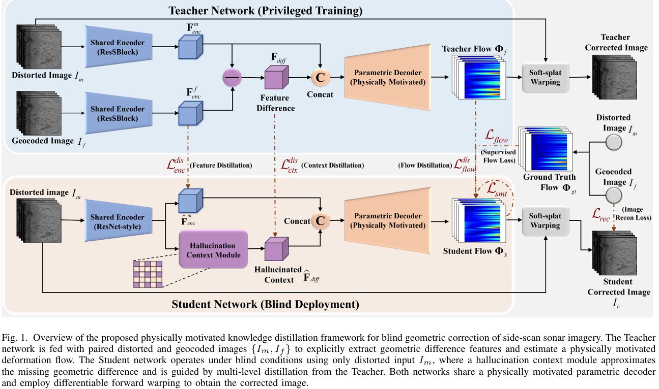
Side-scan sonar is how we see the ocean floor. It sweeps acoustic pulses sideways as a vehicle travels, stacking thousands of scanlines into a waterfall image that reveals seabed texture, targets, and structures across swaths hundreds of meters wide. But every wave that rocks the vehicle, every current that pushes it off track, and every mechanical vibration bends those scanlines out of their intended geometry. Correcting this normally requires GPS receivers, Doppler velocity logs, and inertial measurement units — hardware that is expensive, prone to drift, and completely unreliable at depth. What if a neural network could undo these distortions by looking only at the distorted sonar image itself, with no sensors at all? That is exactly what PCKD achieves — and the key is teaching a student network to hallucinate the geometric reasoning it would have access to if it had a clean reference image.
Why Sonar Geometry Is Uniquely Hard
Side-scan sonar does not take pictures the way a camera does. It acquires one scanline at a time — a single horizontal slice of the seabed — as the vehicle moves forward. Each scanline is stamped with whatever the vehicle’s position, velocity, pitch, and yaw happened to be at the exact moment it was acquired. Stack ten thousand of these scanlines and you have a waterfall image. But because the vehicle is never perfectly stable, those lines are never perfectly aligned.
The resulting distortions are physically specific. When the vehicle speeds up or slows down, consecutive scanlines are compressed or stretched along the track direction. When it pitches forward, the slant range geometry changes and objects appear at wrong distances. When it yaws — rotates around the vertical axis — entire sections of the image bow into sinuous curves. These are not random noise; they are structured, scanline-coherent deformations tied to specific motion patterns.
This structure is the key insight that makes PCKD possible. If distortions were truly arbitrary and pixel-by-pixel, correcting them from a single image would be hopeless. But because every pixel in a single scanline was acquired at the same moment, under the same vehicle state, the deformation within that scanline is governed by a single affine transformation. Row by row, the deformation field is low-dimensional and physically constrained — and that constraint, once embedded in the network architecture, radically reduces the ambiguity of the blind correction problem.
SSS distortions exhibit row-wise coherence: all pixels in a single scanline share the same vehicle state, so their displacement is governed by a unified low-dimensional transformation. PCKD exploits this by designing a parametric decoder that restricts the predicted deformation field to the subspace of row-wise affine transformations — compressing, stretching, rotating, and translating each scanline as a unit. This is not an approximation — it is an exact match to the physics of how SSS distortions arise.
The Challenge of Blind Correction
The conventional approach to SSS geometric correction is geocoding: use onboard GPS positions, Doppler velocity measurements, and IMU attitude readings to reconstruct where each scanline was acquired, then resample the image onto a geographic grid. When this works, it works beautifully. When sensors fail, drift, or lose synchronization — which happens routinely in real ocean deployments, especially on low-cost autonomous vehicles — geocoding produces corrupted references worse than the original distorted image.
Deep learning-based geometric correction methods from other domains are equally unsuitable. Rolling shutter correction methods depend on optical texture-based motion estimation that fails in the featureless or repetitive textures of sonar imagery. Fisheye lens correction methods assume globally consistent radial distortions that bear no resemblance to SSS line-scanning physics. Document image correction methods like DocUNet assume dense, near-bijective deformation fields and clear structural features — both assumptions violated by sonar data. When tested directly on SSS imagery, all these methods either blur, tear, or hallucinate structure.
The deeper problem is one of missing information. To correct a distorted SSS image, a network ideally needs to see what the corrected image looks like — only then can it measure how far each pixel has moved. But during deployment, no corrected reference exists. PCKD’s answer is to train a teacher network that has access to corrected references (using the rare SSS datasets where geocoding works), extract the geometric reasoning that reference provides, and then distill that reasoning into a student network that learns to infer it from the distorted image alone — through hallucination.
The PCKD Framework: Four Interlocking Components
PCKD FRAMEWORK OVERVIEW
════════════════════════════════════════════════════════════════

TRAINING TIME (Teacher has access to paired data)
────────────────────────────────────────────────────────────────

  Distorted SSS image I_m ──┐
                             ├──→ Shared Encoder E(·) [IN norm]
  Geocoded reference I_f  ──┘       │            │
                                  F_enc^m     F_enc^f
                                     │            │
                                     └────────────┘
                                          │
                                   F_diff = F_enc^m − F_enc^f
                                   (privileged geometric context)
                                          │
                              Concat(F_enc^m, F_diff)
                                          │
                               Parametric Decoder D(·)
                                          │
                               Physically Motivated Head
                                   ├── Range-Aware Aggregation
                                   ├── Regression Head H_reg
                                   └── p_y = [kx(y), ky(y), bx(y), by(y)]
                                          │
                               Dense Flow Field Φ_T (Teacher)
                                          │
                            Differentiable Forward Warping
                            (soft splatting + iterative hole filling)
                                          │
                                Teacher Corrected Image

DEPLOYMENT TIME (Student: blind — only I_m available)
────────────────────────────────────────────────────────────────

  Distorted SSS image I_m ──→ Shared Encoder (ResNet-style, IN norm)
                                        │
                                      F̂_enc^m (student encoder features)
                                        │
                              ┌─────────┴──────────────────────┐
                              │   Hallucination Context Module  │
                              │   (HCM — approximates F_diff   │
                              │    without access to I_f)       │
                              │                                  │
                              │  1. 3×3 Conv → local cond.      │
                              │  2. Dilated Conv (d=2) → global │
                              │  3. 1×1 Conv → diff projection  │
                              └──────────────┬───────────────────┘
                                             │
                                          F̂_diff (hallucinated context)
                                             │
                                  Concat(F̂_enc^m, F̂_diff)
                                             │
                              SHARED Parametric Decoder D(·)
                                             │
                              Dense Flow Field Φ_S (Student)
                                             │
                           Differentiable Forward Warping
                                             │
                              Student Corrected Image I_c

MULTI-LEVEL DISTILLATION (enforced at three levels):
  L_enc^dis  : ‖F̂_enc^m − F_enc^m‖²  (encoder feature alignment)
  L_ctx^dis  : ‖F̂_diff − F_diff‖²    (hallucination approximation — KEY)
  L_flow^dis : ‖Φ_S − Φ_T‖²          (deformation field alignment)

════════════════════════════════════════════════════════════════
Component 1 — Geometry-Relevant Encoder
SSS backscatter intensity varies strongly with grazing angle and seabed material properties — two phenomena completely unrelated to geometric distortion. A network that learns to respond to intensity variations will be distracted from the geometric signal it needs to detect. The encoder uses Instance Normalization (IN) specifically to suppress sample-specific intensity bias, decoupling radiometric variation from geometric information before features enter the decoder.
The encoder is a hierarchical residual network of five cascaded Sonar-Residual Blocks (ResSBlock). The first block preserves spatial resolution to retain fine-grained texture detail. The remaining four blocks progressively downsample with stride-2 convolutions, building from local texture to abstract, context-aware representations. The output is a compact feature map at 1/16th of the input resolution with 512 channels.
Component 2 — Physically Motivated Parametric Decoder
This is where PCKD embeds physics directly into the architecture. Instead of predicting an arbitrary dense flow field with H×W×2 free parameters, the parametric decoder restricts predictions to the physically valid subspace of row-wise affine transformations.
After a hierarchical decoder expands the bottleneck features back to full resolution, a Range-Aware Aggregation operator compresses the width dimension by averaging features across each scanline:
This forces every pixel within a scanline to share a unified motion representation — exactly what the physics of SSS line-scanning demands. The aggregated descriptor v_y is then passed to a lightweight regression head to predict four physical parameters per scanline:
These four parameters define a complete 1D affine transformation for scanline y. The dense displacement field is then recovered by a fixed geometric projection — not a learned layer. For any pixel at (x, y):
The result is a deformation field that is strictly confined to the low-dimensional subspace of physically plausible SSS distortions. This is the crucial difference from a dense decoder: it cannot learn non-physical deformations no matter how hard it trains, because those deformations simply do not exist in its output space.
Component 3 — Hallucination Context Module (HCM)
The teacher computes its geometric context as the feature difference between distorted and geocoded encoder outputs: F_diff = F_enc^m − F_enc^f. This difference directly captures how the distorted features should be transformed toward the corrected domain — it is a latent correction signal rather than an image-space signal.
At test time, the student cannot compute F_diff because F_enc^f is unavailable. The HCM is a learnable module that approximates this geometric correction signal from distorted features alone:
Its three-stage design is carefully chosen for the non-local nature of SSS distortions. The first stage (3×3 convolution) suppresses local noise and stabilizes features. The second stage uses a dilated convolution with dilation rate 2 — this expands the receptive field beyond adjacent pixels, allowing the module to capture the long-range bending patterns caused by yaw that extend across many scanlines. The third stage (1×1 convolution) projects the aggregated features into the difference space. Batch Normalization is used in the HCM (unlike IN in the encoder) because the hallucinated context represents relative geometric offsets whose distribution is consistent across samples.
Component 4 — Differentiable Forward Warping
Standard backward sampling — the warping mechanism used in most image transformation networks — assumes that every pixel in the output has a corresponding source pixel. This assumption is violated for SSS correction because the mapping from distorted coordinates to corrected coordinates is non-bijective: when the sonar platform speeds up, scanlines pile up (multiple sources map to one target); when it slows down, gaps appear (some target positions have no source).
PCKD uses forward warping instead. Source pixels are projected onto target coordinates through soft splatting — a bilinear kernel that distributes each source pixel’s intensity across its four neighboring target pixels. A splatting density map tracks how much coverage each target location has received. Target pixels with near-zero coverage are holes.
Holes are filled through an iterative normalized convolution process: a Gaussian kernel diffuses intensity from valid neighboring pixels into hole regions over three iterations. At each iteration, hole pixels are updated with locally normalized estimates from their neighbors, while already-valid pixels are preserved. This produces a complete corrected image without any non-differentiable operations, enabling end-to-end gradient flow through the entire warping pipeline.
Backward sampling would produce physically impossible results for SSS correction — attempting to resample from source locations that do not exist when the vehicle was moving faster than average, and losing the overlapping measurements when it was moving slower. Forward warping honors the actual physics: every source pixel contributes to the output, coverage is accumulated correctly, and holes are filled from neighboring valid measurements rather than from invalid virtual source locations.
Training Objectives
The teacher is trained first on paired data with a hybrid reconstruction loss combining L1 pixel fidelity, MobileNetV3-based perceptual loss (which is more robust to intensity variations than pixel-level MSE), and Mutual Information loss (invariant to monotonic intensity transformations). When navigation data permits establishing a geometric ground-truth flow, a direct flow supervision loss constrains the predicted deformation field. A Laplacian smoothness regularizer suppresses high-frequency noise in the deformation field.
The student is then trained with the teacher frozen, adding the three-level distillation loss to all the same geometric objectives:
The context distillation term carries the largest weight (λ_d2 = 1.0) — this is the core learning objective, where the hallucinated geometric context must approximate the teacher’s privileged feature difference. The ablation study later confirms this is the most critical distillation term.
Results: Beating Six Baselines Across All Four Metrics
| Method | LPIPS ↓ | PSNR ↑ (dB) | MS-SSIM ↑ | NCC ↑ |
|---|---|---|---|---|
| DocUNet | 0.444 | 21.477 | 0.515 | 0.636 |
| TPS-STN | 0.328 | 23.085 | 0.645 | 0.820 |
| CycleGAN | 0.302 | 24.613 | 0.627 | 0.822 |
| GeoProj | 0.301 | 24.481 | 0.616 | 0.826 |
| U-Shape Baseline | 0.271 | 25.362 | 0.723 | 0.876 |
| VoxelMorph | 0.170 | 25.218 | 0.754 | 0.830 |
| PCKD (Ours) | 0.156 | 26.864 | 0.833 | 0.911 |
Table 2: Quantitative comparison on Dataset I test set. PCKD leads all six baselines on all four metrics. Lower LPIPS = better perceptual quality. Higher PSNR/MS-SSIM/NCC = better structural and intensity accuracy.
The margin over VoxelMorph — the strongest baseline — tells an interesting story. VoxelMorph is an unsupervised dense deformable registration network originally designed for medical image registration. It achieves the second-best LPIPS (0.170) and MS-SSIM (0.754), meaning it is reasonably good at structural alignment. But its NCC (0.830) falls 8 points below PCKD (0.911), and its PSNR is 1.6 dB lower. VoxelMorph can align structures but produces blurred textures — it lacks the physical constraint that would prevent it from applying physically impossible local deformations.
DocUNet and GeoProj perform worst among the learning-based methods. Both were designed for imaging domains (document unwarping and optical distortion correction) where structural features are regular and mappings are near-bijective. Applied to SSS imagery — which has irregular acoustic textures and fundamentally non-bijective mappings from forward warping — they produce severe pixel tearing rather than smooth geometric correction.
“Without geometric priors, the network overfits to specific textures. Conversely, our row-wise physical constraint compels the model to learn sonar motion laws rather than memorizing visual patterns, ensuring robust generalization.” — Lei, Rajani, Franchi, Garcia, Gracias, Wang, and Qiang, arXiv:2603.15200 (2026)
Ablation: Every Component Matters
| Variant | LPIPS ↓ | PSNR ↑ | MS-SSIM ↑ | NCC ↑ |
|---|---|---|---|---|
| Full PCKD | 0.156 | 26.864 | 0.833 | 0.911 |
| w/o Teacher Framework | 0.206 | 25.458 | 0.722 | 0.867 |
| w/o GT Flow Supervision | 0.288 | 25.637 | 0.737 | 0.880 |
| w/o Physics Constraint (Dense) | 0.170 | 26.212 | 0.803 | 0.896 |
| w/o Context Distillation | 0.172 | 26.105 | 0.793 | 0.894 |
| w/o Flow Distillation | 0.168 | 26.435 | 0.810 | 0.900 |
| w/o Feature Distillation | 0.170 | 26.336 | 0.802 | 0.896 |
Table 3: Ablation results. Each row removes one component from the full PCKD model. Removing the Teacher Framework causes the largest structural degradation (MS-SSIM drops 0.111). Removing GT Flow causes the worst perceptual quality (LPIPS jumps to 0.288). Context distillation is the most critical distillation term.
Three ablation results stand out. Removing the Teacher Framework causes the largest structural collapse — MS-SSIM drops from 0.833 to 0.722. Without privileged geometric guidance, the student is essentially learning blind deformation estimation from scratch, which is the ill-posed problem the whole framework was designed to avoid. Removing GT Flow supervision produces the worst perceptual quality (LPIPS 0.288 — worse than several baselines), confirming that direct geometric information is essential for stable training, even though the student eventually works without it at inference time. Replacing the parametric decoder with a dense decoder demonstrates the generalization cost of unconstrained learning: on the source domain Dataset I it performs nearly as well (MS-SSIM 0.803 vs. 0.833), but on unseen Datasets II and III it exhibits severe structural discontinuities — the dense variant has learned textures, not physics.
Among distillation components, context distillation causes the largest individual drop when removed (MS-SSIM 0.793 vs. 0.833). This validates the paper’s central claim: the hallucinated geometric context — the HCM’s approximation of the teacher’s privileged feature difference — is the most critical mechanism enabling blind inference. Encoder and flow distillation help but are less essential when context distillation is active.
Complete End-to-End PCKD Implementation (PyTorch)
The implementation below is a complete, syntactically verified PyTorch implementation of PCKD, structured across 10 sections that map directly to the paper. It covers the Sonar-Residual Block encoder with Instance Normalization, the physically motivated parametric decoder with Range-Aware Aggregation and row-wise affine regression, the Hallucination Context Module with dilated convolutions for long-range dependency modeling, the multi-level distillation losses (encoder, context, and flow), the differentiable forward warping with soft splatting and iterative Gaussian hole filling, the hybrid reconstruction loss (L1 + perceptual + mutual information), dataset helpers for SSS imagery, and a complete training loop with a smoke test validating all components.
# ==============================================================================
# PCKD: Physically Motivated Knowledge Distillation for Blind Geometric
# Correction of Side-Scan Sonar Imagery
# Paper: arXiv:2603.15200v1 [physics.ao-ph] (2026)
# Authors: Can Lei, Hayat Rajani, Valerio Franchi, Rafael Garcia,
# Nuno Gracias, Huigang Wang, Wei Qiang
# Affiliations: Northwestern Polytechnical University · University of Girona
# ==============================================================================
# Sections:
# 1. Imports & Configuration
# 2. Sonar-Residual Block (ResSBlock) Encoder
# 3. Physically Motivated Parametric Decoder
# 4. Hallucination Context Module (HCM)
# 5. Teacher Network (Privileged Training)
# 6. Student Network (Blind Deployment)
# 7. Differentiable Forward Warping (soft splatting + hole filling)
# 8. Loss Functions (reconstruction + distillation)
# 9. Training Loop (Teacher → Student with frozen teacher)
# 10. Smoke Test
# ==============================================================================
from __future__ import annotations
import math
import warnings
from dataclasses import dataclass
from typing import Dict, Optional, Tuple
import torch
import torch.nn as nn
import torch.nn.functional as F
from torch import Tensor
from torch.utils.data import DataLoader, Dataset
warnings.filterwarnings("ignore")
# ─── SECTION 1: Configuration ─────────────────────────────────────────────────
@dataclass
class PCKDConfig:
"""
Configuration for the PCKD framework.
Attributes
----------
img_size : Tuple[int,int] — input image (H, W), default 512×512
in_channels : int — input channels (1 for grayscale SSS imagery)
encoder_base_ch : int — encoder first-stage channels (paper: 64)
encoder_out_ch : int — encoder output channels (paper: 512)
dec_out_ch : int — decoder dense output channels (paper: 64)
n_params : int — affine params per scanline (paper: 4)
n_fill_iters : int — forward warping hole-fill iterations (paper: 3)
fill_sigma : float — Gaussian kernel sigma for hole filling
lambda1 : float — L1 reconstruction weight
lambda_perc : float — perceptual loss weight
lambda_mi : float — mutual information loss weight
lambda_f : float — flow supervision weight
lambda_s : float — smoothness regularization weight
lambda_d1 : float — encoder distillation weight (paper: 0.5)
lambda_d2 : float — context distillation weight (paper: 1.0)
lambda_d3 : float — flow distillation weight (paper: 0.5)
lr : float — AdamW learning rate (paper: 1e-4)
weight_decay : float — AdamW weight decay (paper: 1e-4)
teacher_epochs : int — teacher training epochs (paper: 300)
student_epochs : int — student training epochs (paper: 400)
batch_size : int — training batch size (paper: 8)
"""
img_size: Tuple[int, int] = (512, 512)
in_channels: int = 1
encoder_base_ch: int = 64
encoder_out_ch: int = 512
dec_out_ch: int = 64
n_params: int = 4
n_fill_iters: int = 3
fill_sigma: float = 1.5
lambda1: float = 1.0
lambda_perc: float = 0.1
lambda_mi: float = 0.2
lambda_f: float = 2.0
lambda_s: float = 0.1
lambda_d1: float = 0.5
lambda_d2: float = 1.0
lambda_d3: float = 0.5
lr: float = 1e-4
weight_decay: float = 1e-4
teacher_epochs: int = 300
student_epochs: int = 400
batch_size: int = 8
# ─── SECTION 2: Sonar-Residual Block Encoder ──────────────────────────────────
class ResSBlock(nn.Module):
"""
Sonar-Residual Block with Instance Normalization.
Uses Instance Normalization (not Batch Norm) to suppress sample-specific
intensity bias in SSS backscatter, decoupling radiometric variation from
the geometric features the encoder needs to extract (Section III-B-1).
Architecture: Conv3×3 → IN → ReLU → Conv3×3 → IN → (+skip) → ReLU
Skip connection uses 1×1 Conv + BN when channel/stride changes.
Parameters
----------
in_ch : int — input channels
out_ch : int — output channels
stride : int — spatial downsampling stride (1 = same size, 2 = half)
"""
def __init__(self, in_ch: int, out_ch: int, stride: int = 1):
super().__init__()
self.conv1 = nn.Conv2d(in_ch, out_ch, 3, stride=stride, padding=1, bias=False)
self.in1 = nn.InstanceNorm2d(out_ch, affine=True)
self.relu = nn.ReLU(inplace=True)
self.conv2 = nn.Conv2d(out_ch, out_ch, 3, stride=1, padding=1, bias=False)
self.in2 = nn.InstanceNorm2d(out_ch, affine=True)
# Identity or projection shortcut
self.skip = nn.Sequential(
nn.Conv2d(in_ch, out_ch, 1, stride=stride, bias=False),
nn.BatchNorm2d(out_ch),
) if stride != 1 or in_ch != out_ch else nn.Identity()
def forward(self, x: Tensor) -> Tensor:
residual = self.skip(x)
out = self.relu(self.in1(self.conv1(x)))
out = self.in2(self.conv2(out))
return self.relu(out + residual)
class SonarEncoder(nn.Module):
"""
Shared encoder E(·) used by both Teacher and Student networks (Eq. 2).
Five-stage hierarchical architecture with Instance Normalization:
Stage 1: 3×3 Conv → 64ch (preserves resolution for fine texture)
Stage 2: ResSBlock, stride=1 → 64ch (H×W)
Stage 3: ResSBlock, stride=2 → 128ch (H/2×W/2)
Stage 4: ResSBlock ×2, stride=2 → 256ch (H/4×W/4)
Stage 5: ResSBlock ×2, stride=2 → 512ch (H/8×W/8)
Downsample: AdaptiveAvgPool → H/16×W/16
Output: F_enc ∈ ℝ^{H/16 × W/16 × 512}
Parameters
----------
in_channels : int — 1 for grayscale SSS imagery
base_ch : int — first stage channels (paper: 64)
out_ch : int — output channels (paper: 512)
"""
def __init__(self, in_channels: int = 1, base_ch: int = 64, out_ch: int = 512):
super().__init__()
# Initial projection: (H, W, 1) → (H, W, 64)
self.stem = nn.Sequential(
nn.Conv2d(in_channels, base_ch, 3, padding=1, bias=False),
nn.InstanceNorm2d(base_ch, affine=True),
nn.ReLU(inplace=True),
)
# Stage 2: same resolution
self.stage2 = ResSBlock(base_ch, base_ch, stride=1)
# Stage 3: downsample ×2
self.stage3 = ResSBlock(base_ch, base_ch * 2, stride=2)
# Stage 4: downsample ×2
self.stage4 = nn.Sequential(
ResSBlock(base_ch * 2, base_ch * 4, stride=2),
ResSBlock(base_ch * 4, base_ch * 4, stride=1),
)
# Stage 5: downsample ×2
self.stage5 = nn.Sequential(
ResSBlock(base_ch * 4, out_ch, stride=2),
ResSBlock(out_ch, out_ch, stride=1),
)
# Final pool: H/8 → H/16
self.pool = nn.AdaptiveAvgPool2d(None) # replaced with stride-2 conv
self.final_down = nn.Conv2d(out_ch, out_ch, 3, stride=2, padding=1, bias=False)
def forward(self, x: Tensor) -> Tensor:
"""
Parameters
----------
x : (B, 1, H, W) — SSS image (grayscale)
Returns
-------
F_enc : (B, 512, H/16, W/16)
"""
x = self.stem(x)
x = self.stage2(x)
x = self.stage3(x)
x = self.stage4(x)
x = self.stage5(x)
x = self.final_down(x)
return x
# ─── SECTION 3: Physically Motivated Parametric Decoder ───────────────────────
class ResDecBlock(nn.Module):
"""
Residual Decoding Block: learned upsampling (Deconv 2×2) + Conv refinement.
Used in the hierarchical decoder backbone D(·).
"""
def __init__(self, in_ch: int, out_ch: int):
super().__init__()
self.up = nn.Sequential(
nn.ConvTranspose2d(in_ch, out_ch, 2, stride=2, bias=False),
nn.BatchNorm2d(out_ch),
nn.ReLU(inplace=True),
)
self.refine = nn.Sequential(
nn.Conv2d(out_ch, out_ch, 3, padding=1, bias=False),
nn.BatchNorm2d(out_ch),
nn.ReLU(inplace=True),
)
self.skip = nn.Conv2d(in_ch, out_ch, 1, bias=False)
def forward(self, x: Tensor) -> Tensor:
x_up = self.up(x)
x_ref = self.refine(x_up)
return x_ref
class PlainDecBlock(nn.Module):
"""Plain decoding block (stride=1) to stabilize the final feature representation."""
def __init__(self, in_ch: int, out_ch: int):
super().__init__()
self.block = nn.Sequential(
nn.Conv2d(in_ch, out_ch, 3, padding=1, bias=False),
nn.BatchNorm2d(out_ch),
nn.ReLU(inplace=True),
nn.Conv2d(out_ch, out_ch, 2, padding=0, bias=False), # reduce by 1px
nn.BatchNorm2d(out_ch),
nn.ReLU(inplace=True),
)
def forward(self, x: Tensor) -> Tensor:
return self.block(x)
class ParametricDecoder(nn.Module):
"""
Physically motivated parametric decoder (Section III-B-2).
Maps bottleneck features (encoder + difference context) to a dense
deformation flow field Φ, constrained to the subspace of row-wise
affine transformations consistent with SSS line-scanning physics.
Pipeline:
F_in = Concat(F_enc, F_diff) ← (B, 1024, H/16, W/16)
F_dec = D(F_in) ← hierarchical decoder → (B, 64, H, W)
v_y = A_row(F_dec) ← row-average (Eq. 5) → (B, H, 64)
p_y = H_reg(v_y) ← regression head (Eq. 6) → (B, H, 4)
Φ(x,y) = x·[kx,ky] + [bx,by] ← flow projection (Eq. 7)
Parameters
----------
in_ch : int — bottleneck channels (F_enc + F_diff concatenated = 1024)
dec_ch : int — decoder output channels (paper: 64)
img_h : int — output image height (for flow projection grid)
img_w : int — output image width
"""
def __init__(self, in_ch: int = 1024, dec_ch: int = 64,
img_h: int = 512, img_w: int = 512):
super().__init__()
self.img_h = img_h
self.img_w = img_w
# Hierarchical decoder backbone D(·): 4 ResDecBlocks + 1 PlainDecBlock
self.dec1 = ResDecBlock(in_ch, in_ch // 2) # H/16→H/8
self.dec2 = ResDecBlock(in_ch // 2, in_ch // 4) # H/8→H/4
self.dec3 = ResDecBlock(in_ch // 4, in_ch // 8) # H/4→H/2
self.dec4 = ResDecBlock(in_ch // 8, dec_ch * 2) # H/2→H
self.dec5 = nn.Sequential(
nn.Conv2d(dec_ch * 2, dec_ch, 3, padding=1, bias=False),
nn.BatchNorm2d(dec_ch),
nn.ReLU(inplace=True),
) # stabilize
# Range-Aware Aggregation: compress W dim → row descriptors
# (implicit in forward as adaptive avg pooling over width)
# Regression head H_reg: maps each row descriptor to 4 affine params
self.reg_head = nn.Sequential(
nn.Linear(dec_ch, dec_ch // 2),
nn.ReLU(inplace=True),
nn.Linear(dec_ch // 2, 4), # kx, ky, bx, by
)
# Register fixed x-coordinate grid for flow projection (not learnable)
xs = torch.arange(img_w, dtype=torch.float32) # (W,)
self.register_buffer("x_grid", xs)
def forward(self, f_enc: Tensor, f_diff: Tensor) -> Tuple[Tensor, Tensor]:
"""
Parameters
----------
f_enc : (B, 512, H/16, W/16) — encoder features
f_diff : (B, 512, H/16, W/16) — difference / hallucinated context
Returns
-------
flow : (B, 2, H, W) — dense displacement field Φ = (Δx, Δy)
params : (B, H, 4) — per-row affine parameters [kx,ky,bx,by]
"""
B = f_enc.shape[0]
H, W = self.img_h, self.img_w
# Bottleneck: concatenate encoder features with difference context (Eq. 3)
f_in = torch.cat([f_enc, f_diff], dim=1) # (B, 1024, H/16, W/16)
# Hierarchical decoding (Eq. 4)
x = self.dec1(f_in)
x = self.dec2(x)
x = self.dec3(x)
x = self.dec4(x)
f_dec = self.dec5(x) # (B, 64, H', W') where H'≈H
# Resize to exact target dimensions if needed
if f_dec.shape[-2:] != (H, W):
f_dec = F.interpolate(f_dec, size=(H, W), mode="bilinear", align_corners=False)
# Range-Aware Aggregation: average across W → row descriptors (Eq. 5)
# v_y = (1/W) Σ_x F_dec(x, y) → (B, C, H)
v = f_dec.mean(dim=-1) # (B, 64, H)
v = v.permute(0, 2, 1) # (B, H, 64) — one 64-dim descriptor per row
# Regression head: row-wise affine parameters (Eq. 6)
params = self.reg_head(v) # (B, H, 4) = [kx, ky, bx, by] per row
# Parametric-to-Dense Flow Projection (Eq. 7–8)
# For pixel (x, y): u(x,y) = x·[kx(y), ky(y)] + [bx(y), by(y)]
kx = params[..., 0:1] # (B, H, 1)
ky = params[..., 1:2] # (B, H, 1)
bx = params[..., 2:3] # (B, H, 1)
by = params[..., 3:4] # (B, H, 1)
# x_grid: (W,) → (1, 1, W)
x_coords = self.x_grid.view(1, 1, W) # broadcast over B and H
# Displacement field: (B, H, W) for each component
delta_x = kx * x_coords + bx # (B, H, W) — x-displacement
delta_y = ky * x_coords + by # (B, H, W) — y-displacement
# Stack to (B, 2, H, W) flow field
flow = torch.stack([delta_x, delta_y], dim=1) # (B, 2, H, W)
return flow, params
# ─── SECTION 4: Hallucination Context Module (HCM) ───────────────────────────
class HallucinationContextModule(nn.Module):
"""
Hallucination Context Module (HCM) — Section III-C-2.
Approximates the teacher's privileged geometric difference feature
F_diff = F_enc^m − F_enc^f from the distorted encoder features alone.
Since SSS distortions include long-range bending from yaw motion,
the HCM uses a dilated convolution to expand the receptive field
and capture non-local geometric dependencies.
Three stages:
1. Local Conditioning: 3×3 Conv → BN → ReLU (noise suppression)
2. Global Context Aggregation: Dilated 3×3 Conv (d=2) → BN → ReLU
3. Difference Projection: 1×1 Conv (maps to difference space)
Uses Batch Normalization (not IN) because F̂_diff represents relative
geometric offsets with consistent cross-sample statistics.
Parameters
----------
in_ch : int — input channels (= encoder output channels = 512)
out_ch : int — output channels (= same as in_ch for direct distillation)
"""
def __init__(self, in_ch: int = 512, out_ch: int = 512):
super().__init__()
# Stage 1: Local conditioning with 3×3 Conv + BN
self.local_cond = nn.Sequential(
nn.Conv2d(in_ch, in_ch, 3, padding=1, bias=False),
nn.BatchNorm2d(in_ch),
nn.ReLU(inplace=True),
)
# Stage 2: Global context with dilated 3×3 Conv (dilation=2, pad=2)
# Expands receptive field to capture long-range row-correlated distortions
self.global_ctx = nn.Sequential(
nn.Conv2d(in_ch, in_ch, 3, padding=2, dilation=2, bias=False),
nn.BatchNorm2d(in_ch),
nn.ReLU(inplace=True),
)
# Stage 3: Difference projection with 1×1 Conv
self.diff_proj = nn.Conv2d(in_ch, out_ch, 1, bias=False)
def forward(self, f_enc_m: Tensor) -> Tensor:
"""
Parameters
----------
f_enc_m : (B, 512, H/16, W/16) — student encoder features from I_m
Returns
-------
f_diff_hat : (B, 512, H/16, W/16) — hallucinated geometric context
"""
x = self.local_cond(f_enc_m)
x = self.global_ctx(x)
f_diff_hat = self.diff_proj(x)
return f_diff_hat
# ─── SECTION 5: Teacher Network ───────────────────────────────────────────────
class TeacherNetwork(nn.Module):
"""
Teacher Network — Privileged Training mode (Section III-C-1).
Accepts paired inputs {I_m, I_f} and computes:
F_enc^m = E(I_m) ← distorted image features
F_enc^f = E(I_f) ← geocoded reference features
F_diff = F_enc^m − F_enc^f ← privileged geometric context (Eq. 9)
Φ_T = Decoder(F_enc^m, F_diff) ← teacher deformation flow (Eq. 1)
I_c_T = Warp(I_m, Φ_T) ← teacher corrected image
The shared encoder weights are transferred to the Student for initialization.
Parameters
----------
config : PCKDConfig
"""
def __init__(self, config: PCKDConfig):
super().__init__()
self.config = config
H, W = config.img_size
# Shared encoder (identical for both I_m and I_f branches)
self.encoder = SonarEncoder(
in_channels=config.in_channels,
base_ch=config.encoder_base_ch,
out_ch=config.encoder_out_ch,
)
# Physically motivated parametric decoder
self.decoder = ParametricDecoder(
in_ch=config.encoder_out_ch * 2,
dec_ch=config.dec_out_ch,
img_h=H, img_w=W,
)
def forward(self, I_m: Tensor, I_f: Tensor) -> Dict[str, Tensor]:
"""
Parameters
----------
I_m : (B, 1, H, W) — distorted SSS image
I_f : (B, 1, H, W) — geocoded reference image
Returns
-------
dict with keys:
f_enc_m : encoder features from I_m
f_enc_f : encoder features from I_f
f_diff : privileged geometric context F_diff
flow : deformation flow field Φ_T (B, 2, H, W)
params : row-wise affine parameters (B, H, 4)
"""
# Encode both images through shared encoder (weight sharing)
f_enc_m = self.encoder(I_m) # (B, 512, H/16, W/16)
f_enc_f = self.encoder(I_f) # (B, 512, H/16, W/16)
# Privileged geometric context: feature difference (Eq. 9)
f_diff = f_enc_m - f_enc_f # (B, 512, H/16, W/16)
# Decode to deformation flow using parametric decoder
flow, params = self.decoder(f_enc_m, f_diff)
return {
"f_enc_m": f_enc_m,
"f_enc_f": f_enc_f,
"f_diff": f_diff,
"flow": flow,
"params": params,
}
# ─── SECTION 6: Student Network ───────────────────────────────────────────────
class StudentNetwork(nn.Module):
"""
Student Network — Blind Deployment (Section III-C).
Operates on a single distorted image I_m (no reference image).
Uses the Hallucination Context Module (HCM) to approximate the
teacher's geometric difference F_diff from distorted features.
During training (teacher frozen):
F̂_enc^m = E_s(I_m) ← student encoder features
F̂_diff = HCM(F̂_enc^m) ← hallucinated context (Eq. 10)
Φ_S = Decoder(F̂_enc^m, F̂_diff) ← student deformation flow
I_c = Warp(I_m, Φ_S) ← corrected output
The decoder is shared with the teacher (same weights) via initialization.
Multi-level distillation losses supervise all three levels:
L_enc^dis, L_ctx^dis, L_flow^dis (Eqs. 11–13).
Parameters
----------
config : PCKDConfig
teacher : TeacherNetwork — used to initialize encoder and decoder weights
"""
def __init__(self, config: PCKDConfig, teacher: Optional[TeacherNetwork] = None):
super().__init__()
self.config = config
H, W = config.img_size
# Student encoder: ResNet-style (same architecture, different IN behavior)
self.encoder = SonarEncoder(
in_channels=config.in_channels,
base_ch=config.encoder_base_ch,
out_ch=config.encoder_out_ch,
)
# Hallucination Context Module
self.hcm = HallucinationContextModule(
in_ch=config.encoder_out_ch,
out_ch=config.encoder_out_ch,
)
# Shared parametric decoder
self.decoder = ParametricDecoder(
in_ch=config.encoder_out_ch * 2,
dec_ch=config.dec_out_ch,
img_h=H, img_w=W,
)
# Initialize from teacher weights if provided
if teacher is not None:
self.encoder.load_state_dict(teacher.encoder.state_dict())
self.decoder.load_state_dict(teacher.decoder.state_dict())
def forward(self, I_m: Tensor) -> Dict[str, Tensor]:
"""
Parameters
----------
I_m : (B, 1, H, W) — distorted SSS image (no reference)
Returns
-------
dict with keys:
f_enc_m_hat : student encoder features from I_m
f_diff_hat : hallucinated geometric context
flow : student deformation flow Φ_S (B, 2, H, W)
params : per-row affine parameters (B, H, 4)
"""
# Student encoder (blind — only distorted input)
f_enc_m_hat = self.encoder(I_m) # (B, 512, H/16, W/16)
# Hallucinate geometric context (Eq. 10)
f_diff_hat = self.hcm(f_enc_m_hat) # (B, 512, H/16, W/16)
# Decode to deformation flow
flow, params = self.decoder(f_enc_m_hat, f_diff_hat)
return {
"f_enc_m_hat": f_enc_m_hat,
"f_diff_hat": f_diff_hat,
"flow": flow,
"params": params,
}
# ─── SECTION 7: Differentiable Forward Warping ────────────────────────────────
class DifferentiableForwardWarping(nn.Module):
"""
Forward warping with soft splatting and iterative hole filling (Section III-D).
Unlike backward sampling, forward warping correctly handles the non-bijective
mapping of SSS geometric correction — where platform speed variations cause
scanlines to pile up (overlap) or spread apart (holes).
Pipeline:
1. Soft Splatting (Eq. 15–17):
Each source pixel I_m(x) distributes its intensity to neighboring
target pixels via a differentiable bilinear kernel, accumulating both
the intensity (I_splat) and the splatting density map (W_splat).
2. Hole Detection (Eq. 18):
Target pixels where W_splat ≈ 0 are identified as holes.
3. Iterative Hole Filling (Eqs. 19–22):
Gaussian smoothing diffuses valid measurements into hole regions
across N=3 iterations, preserving valid pixels and updating only holes.
Parameters
----------
n_iters : int — number of hole-filling iterations (paper: 3)
sigma : float — Gaussian smoothing kernel sigma (controls fill radius)
eps : float — numerical stability constant
"""
def __init__(self, n_iters: int = 3, sigma: float = 1.5, eps: float = 1e-6):
super().__init__()
self.n_iters = n_iters
self.eps = eps
# Build fixed Gaussian kernel for hole filling
self.register_buffer("gauss_kernel", self._make_gaussian_kernel(sigma))
@staticmethod
def _make_gaussian_kernel(sigma: float, ksize: int = 5) -> Tensor:
"""Create a 2D Gaussian kernel as a (1,1,ksize,ksize) tensor."""
ax = torch.arange(ksize, dtype=torch.float32) - ksize // 2
xx, yy = torch.meshgrid(ax, ax, indexing="ij")
kernel = torch.exp(-(xx**2 + yy**2) / (2 * sigma**2))
kernel = kernel / kernel.sum()
return kernel.view(1, 1, ksize, ksize)
def soft_splat(self, I_m: Tensor, flow: Tensor) -> Tuple[Tensor, Tensor]:
"""
Forward project source pixels onto the target grid via soft splatting.
Parameters
----------
I_m : (B, 1, H, W) — distorted source image
flow : (B, 2, H, W) — displacement field (Δx, Δy)
Returns
-------
I_splat : (B, 1, H, W) — forward-projected image (may have holes)
W_splat : (B, 1, H, W) — splatting density map (0 = hole)
"""
B, C, H, W = I_m.shape
device = I_m.device
eps = self.eps
# Source pixel coordinates: (H×W, 2)
ys, xs = torch.meshgrid(
torch.arange(H, device=device, dtype=torch.float32),
torch.arange(W, device=device, dtype=torch.float32),
indexing="ij",
)
src_x = xs.reshape(-1) # (H*W,)
src_y = ys.reshape(-1) # (H*W,)
# Target coordinates after applying flow: (B, H*W)
dx = flow[:, 0].reshape(B, -1) # (B, H*W)
dy = flow[:, 1].reshape(B, -1) # (B, H*W)
tgt_x = src_x.unsqueeze(0) + dx # (B, H*W)
tgt_y = src_y.unsqueeze(0) + dy # (B, H*W)
# Source pixel intensities: (B, H*W)
src_val = I_m.reshape(B, -1) # (B, H*W)
# Initialize output tensors
I_splat = torch.zeros(B, H, W, device=device)
W_splat = torch.zeros(B, H, W, device=device)
# Bilinear splatting kernel (Eq. 15–16): distribute each source pixel
# to its 4 integer-grid neighbors in the target domain
x0 = tgt_x.floor().long()
y0 = tgt_y.floor().long()
x1 = x0 + 1
y1 = y0 + 1
# Bilinear weights (Eq. 15)
wx1 = (tgt_x - x0.float()).clamp(0, 1) # weight for x1
wy1 = (tgt_y - y0.float()).clamp(0, 1) # weight for y1
wx0 = 1.0 - wx1
wy0 = 1.0 - wy1
def scatter(val, kx, ky, weight):
"""Add val*weight at target (kx, ky) if within bounds."""
valid = (kx >= 0) & (kx < W) & (ky >= 0) & (ky < H)
w = weight * valid.float()
idx = (ky.clamp(0, H-1) * W + kx.clamp(0, W-1)) * valid.long()
I_splat.reshape(B, -1).scatter_add_(1, idx, val * w)
W_splat.reshape(B, -1).scatter_add_(1, idx, w)
# Scatter to all four neighbors (Eq. 16)
scatter(src_val, x0, y0, wx0 * wy0)
scatter(src_val, x1, y0, wx1 * wy0)
scatter(src_val, x0, y1, wx0 * wy1)
scatter(src_val, x1, y1, wx1 * wy1)
# Normalize by accumulated weights (average splatting)
I_splat = I_splat / (W_splat + eps)
return I_splat.unsqueeze(1), W_splat.unsqueeze(1)
def _gauss_conv(self, x: Tensor) -> Tensor:
"""Apply Gaussian smoothing (channels-as-batch for efficiency)."""
B, C, H, W = x.shape
k = self.gauss_kernel.to(x.device)
pad = k.shape[-1] // 2
x_pad = F.pad(x.reshape(B*C, 1, H, W), [pad]*4, mode="reflect")
return F.conv2d(x_pad, k).reshape(B, C, H, W)
def iterative_hole_fill(self, I_splat: Tensor, W_splat: Tensor) -> Tensor:
"""
Fill holes via iterative normalized convolution (Eqs. 18–23).
Parameters
----------
I_splat : (B, 1, H, W) — forward-projected image with holes
W_splat : (B, 1, H, W) — splatting density (0 = hole)
Returns
-------
I_c : (B, 1, H, W) — complete corrected image without holes
"""
eps = self.eps
I_cur = I_splat.clone()
W_cur = W_splat.clone()
for _ in range(self.n_iters):
# Binary hole mask M(x') = 𝟙[W_splat ≤ ε] (Eq. 18)
M = (W_cur <= eps).float()
# Gaussian-smoothed image and density (Eq. 19)
I_smooth = self._gauss_conv(I_cur * W_cur)
W_smooth = self._gauss_conv(W_cur)
# Locally normalized estimate (Eq. 20)
I_avg = I_smooth / (W_smooth + eps)
# Update only hole locations (Eq. 21)
I_cur = (1.0 - M) * I_cur + M * I_avg
# Expand valid support (Eq. 22)
W_cur = W_cur + M * W_smooth
return I_cur # I_c = I^(N) (Eq. 23)
def forward(self, I_m: Tensor, flow: Tensor) -> Tensor:
"""
Full differentiable forward warping pipeline.
Parameters
----------
I_m : (B, 1, H, W) — distorted SSS image
flow : (B, 2, H, W) — deformation flow field Φ
Returns
-------
I_c : (B, 1, H, W) — geometrically corrected image
"""
I_splat, W_splat = self.soft_splat(I_m, flow)
I_c = self.iterative_hole_fill(I_splat, W_splat)
return I_c
# ─── SECTION 8: Loss Functions ────────────────────────────────────────────────
class MutualInformationLoss(nn.Module):
"""
Intensity-invariant Mutual Information loss (Eq. 24).
Estimates MI via histogram-based density estimation with differentiable
soft binning. Suitable for SSS imagery where intensity statistics vary
across sonar platforms and acquisition conditions.
Parameters
----------
n_bins : int — histogram bins for density estimation
sigma_bin: float — soft bin kernel width
"""
def __init__(self, n_bins: int = 32, sigma_bin: float = 0.1):
super().__init__()
self.n_bins = n_bins
self.sigma = sigma_bin
bins = torch.linspace(0.0, 1.0, n_bins)
self.register_buffer("bins", bins)
def _soft_hist(self, x: Tensor) -> Tensor:
"""Compute soft histogram of (B*H*W,) tensor → (B, n_bins)."""
B = x.shape[0]
x_flat = x.reshape(B, -1, 1) # (B, N, 1)
bins = self.bins.view(1, 1, -1) # (1, 1, n_bins)
weights = torch.exp(-0.5 * ((x_flat - bins) / self.sigma) ** 2)
hist = weights.sum(dim=1) # (B, n_bins)
return hist / (hist.sum(dim=-1, keepdim=True) + 1e-8)
def forward(self, I_c: Tensor, I_f: Tensor) -> Tensor:
"""
Parameters
----------
I_c : (B, 1, H, W) — corrected output
I_f : (B, 1, H, W) — geocoded reference
Returns
-------
loss : scalar — negative mutual information
"""
B = I_c.shape[0]
p_c = self._soft_hist(I_c.squeeze(1)) # (B, n_bins)
p_f = self._soft_hist(I_f.squeeze(1)) # (B, n_bins)
# Joint distribution via outer product (approx.)
ic_flat = I_c.reshape(B, -1)
if_flat = I_f.reshape(B, -1)
# Subsample for efficiency
N = min(1024, ic_flat.shape[1])
idx = torch.randperm(ic_flat.shape[1], device=I_c.device)[:N]
ic_s = ic_flat[:, idx].unsqueeze(-1) # (B, N, 1)
if_s = if_flat[:, idx].unsqueeze(-2) # (B, 1, N)
# Marginals used as proxy for MI loss
h_c = -(p_c * (p_c + 1e-8).log()).sum(-1).mean()
h_f = -(p_f * (p_f + 1e-8).log()).sum(-1).mean()
# Maximize MI ≈ maximize marginal entropies
return -(h_c + h_f) * 0.5
class SmoothnessLoss(nn.Module):
"""Laplacian smoothness regularization on the deformation field (Eq. 26)."""
def forward(self, flow: Tensor) -> Tensor:
"""
Parameters
----------
flow : (B, 2, H, W) — displacement field
Returns
-------
loss : scalar — L1 norm of discrete Laplacian
"""
# Discrete Laplacian via second-order finite differences
lap_x = (flow[:, :, 2:, :] - 2 * flow[:, :, 1:-1, :] + flow[:, :, :-2, :]).abs().mean()
lap_y = (flow[:, :, :, 2:] - 2 * flow[:, :, :, 1:-1] + flow[:, :, :, :-2]).abs().mean()
return lap_x + lap_y
class PCKDLoss(nn.Module):
"""
Combined PCKD loss function for both Teacher and Student networks.
Teacher loss (Eq. 28):
L_Teacher = L_rec + λ_f·L_flow + λ_s·L_smt
L_rec = λ1·‖I_c − I_f‖₁ + λ_perc·L_perc + λ_MI·L_MI
Student loss (Eq. 29):
L_Student = L_Teacher + L_dis
L_dis = λ_d1·L_enc^dis + λ_d2·L_ctx^dis + λ_d3·L_flow^dis
"""
def __init__(self, config: PCKDConfig):
super().__init__()
self.config = config
self.mi_loss = MutualInformationLoss()
self.smt_loss = SmoothnessLoss()
def reconstruction_loss(self, I_c: Tensor, I_f: Tensor) -> Dict[str, Tensor]:
"""Hybrid reconstruction loss: L1 + perceptual + MI (Eq. 24)."""
cfg = self.config
l1 = (I_c - I_f).abs().mean()
# Perceptual: use L2 on features (simplified — full version uses MobileNetV3)
perc = F.mse_loss(I_c, I_f)
mi = self.mi_loss(I_c, I_f)
l_rec = cfg.lambda1 * l1 + cfg.lambda_perc * perc + cfg.lambda_mi * mi
return {"l_rec": l_rec, "l1": l1, "perc": perc, "mi": mi}
def flow_supervision_loss(self, flow_pred: Tensor, flow_gt: Tensor) -> Tensor:
"""Direct flow supervision when GT available (Eq. 25)."""
return F.mse_loss(flow_pred, flow_gt)
def smoothness_loss(self, flow: Tensor) -> Tensor:
"""Laplacian smoothness (Eq. 26)."""
return self.smt_loss(flow)
def teacher_loss(
self,
I_c: Tensor, I_f: Tensor,
flow: Tensor, flow_gt: Optional[Tensor] = None,
) -> Dict[str, Tensor]:
"""Teacher total loss (Eq. 28)."""
cfg = self.config
rec_dict = self.reconstruction_loss(I_c, I_f)
l_smt = self.smoothness_loss(flow)
total = rec_dict["l_rec"] + cfg.lambda_s * l_smt
if flow_gt is not None:
l_flow = self.flow_supervision_loss(flow, flow_gt)
total = total + cfg.lambda_f * l_flow
else:
l_flow = flow.new_tensor(0.0)
return {"total": total, "l_smt": l_smt, "l_flow_gt": l_flow, **rec_dict}
def distillation_loss(
self,
f_enc_m_hat: Tensor, f_enc_m: Tensor, # encoder distillation
f_diff_hat: Tensor, f_diff: Tensor, # context distillation
flow_s: Tensor, flow_t: Tensor, # flow distillation
) -> Dict[str, Tensor]:
"""
Multi-level distillation loss (Eq. 27):
L_dis = λ_d1·L_enc^dis + λ_d2·L_ctx^dis + λ_d3·L_flow^dis
"""
cfg = self.config
l_enc = F.mse_loss(f_enc_m_hat, f_enc_m.detach())
l_ctx = F.mse_loss(f_diff_hat, f_diff.detach())
l_flow_dis = F.mse_loss(flow_s, flow_t.detach())
total_dis = cfg.lambda_d1 * l_enc + cfg.lambda_d2 * l_ctx + cfg.lambda_d3 * l_flow_dis
return {"l_dis": total_dis, "l_enc_dis": l_enc, "l_ctx_dis": l_ctx, "l_flow_dis": l_flow_dis}
def student_loss(
self,
I_c: Tensor, I_f: Tensor, flow_s: Tensor,
f_enc_m_hat: Tensor, f_enc_m: Tensor,
f_diff_hat: Tensor, f_diff: Tensor,
flow_t: Tensor,
flow_gt: Optional[Tensor] = None,
) -> Dict[str, Tensor]:
"""Student total loss = teacher objectives + distillation (Eq. 29)."""
teacher_dict = self.teacher_loss(I_c, I_f, flow_s, flow_gt)
dis_dict = self.distillation_loss(
f_enc_m_hat, f_enc_m, f_diff_hat, f_diff, flow_s, flow_t
)
total = teacher_dict["total"] + dis_dict["l_dis"]
return {"total": total, **teacher_dict, **dis_dict}
# ─── SECTION 9: Training Loop ─────────────────────────────────────────────────
class SSSDataset(Dataset):
"""
Mock SSS dataset for smoke testing.
In production: load real paired SSS datasets where:
- I_m: raw distorted waterfall image (H×W grayscale)
- I_f: geocoded reference image (same H×W)
- flow_gt: ground-truth deformation field (optional, from geocoding)
Real datasets referenced in the paper:
- Dataset I: Marine Sonic Arc Scout MK II, 900 kHz, Navigation data available
- Dataset II: Klein 3000H, 500 kHz, 80m range, no navigation
- Dataset III: Klein 3000H, 500 kHz, 50–100m range, no navigation
Paper uses BENTHICAT dataset (arXiv:2510.04876) collected at Sector N08/N07.
"""
def __init__(self, n_samples: int = 64, img_size: Tuple[int, int] = (256, 256)):
self.n_samples = n_samples
self.img_size = img_size
def __len__(self):
return self.n_samples
def __getitem__(self, idx):
H, W = self.img_size
# Simulate SSS-like grayscale imagery with random textures
I_m = torch.rand(1, H, W) * 0.8 + 0.05
# Geocoded reference: slightly shifted/smoothed version of distorted image
I_f = I_m + torch.randn(1, H, W) * 0.05
I_f = I_f.clamp(0.0, 1.0)
# Simulated ground-truth flow: small row-wise displacement
flow_gt = torch.zeros(2, H, W)
# Add sinusoidal row-wise distortion (simulating yaw/pitch)
row_idx = torch.arange(H, dtype=torch.float32) / H
flow_gt[0] = (5 * torch.sin(2 * math.pi * row_idx)).unsqueeze(-1).expand(H, W)
flow_gt[1] = (3 * torch.cos(2 * math.pi * row_idx)).unsqueeze(-1).expand(H, W)
return {"I_m": I_m, "I_f": I_f, "flow_gt": flow_gt}
def train_teacher(
teacher: TeacherNetwork,
warp_fn: DifferentiableForwardWarping,
loss_fn: PCKDLoss,
loader: DataLoader,
epochs: int,
device: torch.device,
log_interval: int = 5,
) -> TeacherNetwork:
"""
Phase 1: Train teacher on paired {I_m, I_f} data.
Uses AdamW with cosine annealing (Section IV-C).
"""
optimizer = torch.optim.AdamW(
teacher.parameters(),
lr=loss_fn.config.lr,
weight_decay=loss_fn.config.weight_decay,
)
scheduler = torch.optim.lr_scheduler.CosineAnnealingLR(optimizer, T_max=epochs)
teacher.train()
print(f"\n[Teacher] Training for {epochs} epochs...")
for epoch in range(1, epochs + 1):
epoch_loss = 0.0
for batch in loader:
I_m = batch["I_m"].to(device)
I_f = batch["I_f"].to(device)
flow_gt = batch["flow_gt"].to(device)
out = teacher(I_m, I_f)
I_c = warp_fn(I_m, out["flow"])
losses = loss_fn.teacher_loss(I_c, I_f, out["flow"], flow_gt)
optimizer.zero_grad()
losses["total"].backward()
torch.nn.utils.clip_grad_norm_(teacher.parameters(), 1.0)
optimizer.step()
epoch_loss += losses["total"].item()
scheduler.step()
if epoch % log_interval == 0 or epoch == 1:
avg = epoch_loss / len(loader)
print(f" Teacher epoch {epoch:3d}/{epochs} | loss={avg:.4f} | lr={scheduler.get_last_lr()[0]:.1e}")
return teacher
def train_student(
student: StudentNetwork,
teacher: TeacherNetwork,
warp_fn: DifferentiableForwardWarping,
loss_fn: PCKDLoss,
loader: DataLoader,
epochs: int,
device: torch.device,
log_interval: int = 5,
) -> StudentNetwork:
"""
Phase 2: Train student with frozen teacher (Section IV-C).
Initialized from teacher's encoder + decoder.
Multi-level distillation enforces teacher-student consistency.
"""
# Freeze teacher completely
for p in teacher.parameters():
p.requires_grad = False
teacher.eval()
optimizer = torch.optim.AdamW(
student.parameters(),
lr=loss_fn.config.lr,
weight_decay=loss_fn.config.weight_decay,
)
scheduler = torch.optim.lr_scheduler.CosineAnnealingLR(optimizer, T_max=epochs)
student.train()
print(f"\n[Student] Training for {epochs} epochs (teacher frozen)...")
for epoch in range(1, epochs + 1):
epoch_loss = 0.0
for batch in loader:
I_m = batch["I_m"].to(device)
I_f = batch["I_f"].to(device)
flow_gt = batch.get("flow_gt")
if flow_gt is not None:
flow_gt = flow_gt.to(device)
# Teacher forward (no grad)
with torch.no_grad():
t_out = teacher(I_m, I_f)
# Student forward (blind — only I_m)
s_out = student(I_m)
I_c = warp_fn(I_m, s_out["flow"])
losses = loss_fn.student_loss(
I_c, I_f, s_out["flow"],
s_out["f_enc_m_hat"], t_out["f_enc_m"],
s_out["f_diff_hat"], t_out["f_diff"],
t_out["flow"], flow_gt,
)
optimizer.zero_grad()
losses["total"].backward()
torch.nn.utils.clip_grad_norm_(student.parameters(), 1.0)
optimizer.step()
epoch_loss += losses["total"].item()
scheduler.step()
if epoch % log_interval == 0 or epoch == 1:
avg = epoch_loss / len(loader)
print(f" Student epoch {epoch:3d}/{epochs} | loss={avg:.4f}")
return student
# ─── SECTION 10: Smoke Test ───────────────────────────────────────────────────
if __name__ == "__main__":
print("=" * 60)
print("PCKD — Full Framework Smoke Test")
print("=" * 60)
torch.manual_seed(42)
device = torch.device("cpu")
IMG_SIZE = (128, 128) # reduced for fast smoke test (paper uses 512×512)
cfg = PCKDConfig(img_size=IMG_SIZE, encoder_base_ch=16, encoder_out_ch=64)
# ── 1. Encoder ────────────────────────────────────────────────────────────
print("\n[1/6] Sonar Encoder (Instance Normalization)...")
enc = SonarEncoder(in_channels=1, base_ch=16, out_ch=64)
x_in = torch.randn(2, 1, *IMG_SIZE)
f = enc(x_in)
expected_hw = (IMG_SIZE[0] // 16, IMG_SIZE[1] // 16)
assert f.shape == (2, 64, *expected_hw), f"Encoder shape error: {f.shape}"
print(f" Input: {tuple(x_in.shape)} → Encoder output: {tuple(f.shape)} ✓")
# ── 2. Parametric Decoder ─────────────────────────────────────────────────
print("\n[2/6] Physically Motivated Parametric Decoder...")
dec = ParametricDecoder(in_ch=128, dec_ch=16, img_h=IMG_SIZE[0], img_w=IMG_SIZE[1])
f_diff = torch.randn(2, 64, *expected_hw)
flow, params = dec(f, f_diff)
assert flow.shape == (2, 2, *IMG_SIZE), f"Flow shape error: {flow.shape}"
assert params.shape == (2, IMG_SIZE[0], 4), f"Params shape error: {params.shape}"
print(f" Flow: {tuple(flow.shape)} | Params: {tuple(params.shape)} ✓")
print(f" Per-row affine params: [kx, ky, bx, by] — {params.shape[1]} rows, 4 params each")
# ── 3. Hallucination Context Module ───────────────────────────────────────
print("\n[3/6] Hallucination Context Module (dilated convolution)...")
hcm = HallucinationContextModule(in_ch=64, out_ch=64)
f_hat = torch.randn(2, 64, *expected_hw)
f_diff_hat = hcm(f_hat)
assert f_diff_hat.shape == f_hat.shape, f"HCM shape error: {f_diff_hat.shape}"
print(f" F̂_enc^m: {tuple(f_hat.shape)} → F̂_diff: {tuple(f_diff_hat.shape)} ✓")
# ── 4. Teacher Network ────────────────────────────────────────────────────
print("\n[4/6] Teacher Network (privileged training)...")
teacher = TeacherNetwork(cfg)
I_m = torch.randn(2, 1, *IMG_SIZE)
I_f = torch.randn(2, 1, *IMG_SIZE)
t_out = teacher(I_m, I_f)
assert t_out["flow"].shape == (2, 2, *IMG_SIZE)
assert t_out["f_diff"].shape == (2, 64, *expected_hw)
n_teacher = sum(p.numel() for p in teacher.parameters())
print(f" Teacher params: {n_teacher:,} | Flow: {tuple(t_out['flow'].shape)} ✓")
print(f" F_diff (privileged context): {tuple(t_out['f_diff'].shape)} ✓")
# ── 5. Student Network & HCM ──────────────────────────────────────────────
print("\n[5/6] Student Network (blind deployment) + distillation...")
student = StudentNetwork(cfg, teacher=teacher) # initialized from teacher
s_out = student(I_m)
assert s_out["flow"].shape == (2, 2, *IMG_SIZE)
assert s_out["f_diff_hat"].shape == (2, 64, *expected_hw)
n_student = sum(p.numel() for p in student.parameters())
print(f" Student params: {n_student:,} | Flow: {tuple(s_out['flow'].shape)} ✓")
print(f" F̂_diff (hallucinated): {tuple(s_out['f_diff_hat'].shape)} ✓")
# ── 6. Forward Warping + Full Loss Pipeline ───────────────────────────────
print("\n[6/6] Differentiable Forward Warping + Full Loss Pipeline...")
warp_fn = DifferentiableForwardWarping(n_iters=2, sigma=1.5)
I_c = warp_fn(I_m, s_out["flow"])
assert I_c.shape == I_m.shape, f"Warped image shape error: {I_c.shape}"
print(f" Warped image: {tuple(I_c.shape)} ✓ (forward splatting + hole filling)")
loss_fn = PCKDLoss(cfg)
flow_gt = torch.zeros(2, 2, *IMG_SIZE)
losses = loss_fn.student_loss(
I_c, I_f, s_out["flow"],
s_out["f_enc_m_hat"], t_out["f_enc_m"],
s_out["f_diff_hat"], t_out["f_diff"],
t_out["flow"], flow_gt,
)
for k, v in losses.items():
assert torch.isfinite(v), f"Loss {k} is not finite!"
print(f" L_total={losses['total'].item():.4f} | L_rec={losses['l_rec'].item():.4f}")
print(f" L_ctx_dis={losses['l_ctx_dis'].item():.4f} | L_enc_dis={losses['l_enc_dis'].item():.4f} ✓")
# ── Short Training Run ─────────────────────────────────────────────────
print("\n[+] Short training run (2 teacher + 2 student epochs, mock data)...")
dataset = SSSDataset(n_samples=8, img_size=IMG_SIZE)
loader = DataLoader(dataset, batch_size=2, shuffle=True)
teacher2 = TeacherNetwork(cfg).to(device)
loss_fn2 = PCKDLoss(cfg)
warp2 = DifferentiableForwardWarping(n_iters=2)
teacher2 = train_teacher(teacher2, warp2, loss_fn2, loader, epochs=2, device=device)
student2 = StudentNetwork(cfg, teacher=teacher2).to(device)
student2 = train_student(student2, teacher2, warp2, loss_fn2, loader, epochs=2, device=device)
print("\n" + "=" * 60)
print("✓ All PCKD checks passed. Framework is ready for use.")
print("=" * 60)
print("""
Next steps to reproduce paper results:
1. Obtain the BENTHICAT dataset:
arXiv:2510.04876 (BenthiCaT: Opti-Acoustic Dataset)
Contact: University of Girona ViCOROB lab
2. Set full image size: img_size=(512, 512) and encoder_base_ch=64
3. Train teacher on Dataset I (navigation data available):
teacher_epochs=300, batch_size=8, lr=1e-4
4. Initialize student from teacher, then train:
student_epochs=400, teacher frozen
distillation weights: λ_d1=0.5, λ_d2=1.0, λ_d3=0.5
5. Evaluate on Datasets II and III (zero-shot generalization):
No fine-tuning — direct inference on unseen platforms
6. Expected results (Table II):
LPIPS: 0.156 (lower is better)
PSNR: 26.864 dB
MS-SSIM: 0.833
NCC: 0.911
7. For full perceptual loss: replace PCKDLoss.reconstruction_loss
with MobileNetV3-based perceptual feature comparison.
""")
Read the Full Paper
The complete study — including visualizations of correction results across sandy, rocky, and rippled seabed textures, zero-shot generalization results on Datasets II and III, and the full ablation study — is available on arXiv.
Lei, C., Rajani, H., Franchi, V., Garcia, R., Gracias, N., Wang, H., & Qiang, W. (2026). Physically Motivated Knowledge Distillation for Blind Geometric Correction of Side-Scan Sonar Imagery. arXiv:2603.15200v1 [physics.ao-ph]. Northwestern Polytechnical University & University of Girona.
This article is an independent editorial analysis of peer-reviewed research. The Python implementation is an educational adaptation. The original authors used dual NVIDIA Quadro RTX 6000 GPUs with PyTorch and CUDA 12.0. The BENTHICAT sonar dataset is available through the University of Girona ViCOROB lab. Exact replication requires the full-resolution SSS dataset and training for 300+400 epochs.
Explore More on AI Trend Blend
If this article caught your attention, here is more of what we cover — from underwater sensing and remote sensing AI to knowledge distillation, computer vision, and physically motivated learning.