The Moon’s Many Faces: How One Transformer Learned to Speak All Four Languages of Lunar Science Simultaneously
A team at TU Dortmund built a single 29.7-million-parameter foundation model that can translate any combination of lunar data — grayscale images, elevation maps, surface normals, and albedo — to any other, all in a single forward pass. The key insight: Shape and Albedo from Shading is fundamentally a multimodal learning problem.
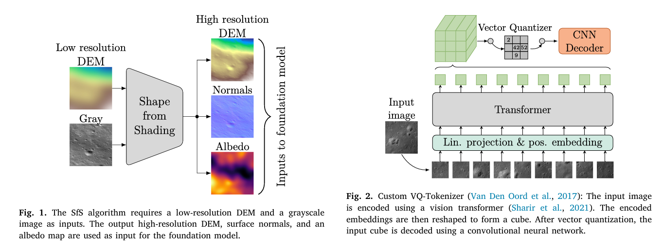
For decades, reconstructing the three-dimensional surface of the Moon from camera images has required either stereoscopic image pairs — expensive and coverage-limited — or a specialized Shape from Shading algorithm that takes hours to run on a single image and requires deep domain expertise to configure. Tom Sander and his colleagues at TU Dortmund ask a different question entirely: what if the problem of joint height and albedo estimation is not a numerical optimization problem at all, but a multimodal learning problem? What if a transformer that understands the relationship between a shadow and an elevation value can do in milliseconds what SfS does in hours?
Why Planetary Reconstruction Is Stuck
The lunar surface is, in terms of raw data volume, one of the best-documented objects in the solar system. The Lunar Reconnaissance Orbiter has been imaging the Moon at 0.5 metres per pixel since 2009. The Lunar Orbiter Laser Altimeter has bounced laser pulses off virtually every square kilometre of the surface. And yet, combining those two data streams into high-resolution, globally consistent DEMs remains enormously expensive — computationally and scientifically.
Stereo vision produces accurate DEMs but needs overlapping image pairs that aren’t always available, and the resulting resolution is typically three to five times coarser than the input images. Laser altimetry gives excellent vertical accuracy but terrible cross-track resolution. Shape from Shading fills the gap in resolution — inferring surface slope from how bright each pixel is under known illumination — but it’s slow, sensitive to initialization, and produces relative heights rather than absolute ones unless anchored to a lower-resolution DEM.
The machine learning community has attacked this with CNNs and GANs over the last few years: models like MADNet and GADEM can generate high-resolution lunar DEMs from single grayscale images in a fraction of the time that SfS takes. They all share one limitation, though. They are specialized for one task — image to DEM — and treat the problem as a supervised regression from a fixed input format to a fixed output format. Want to also estimate albedo? That’s a different model. Want to generate a grayscale image from a DEM? Yet another model.
Rather than building a model for each lunar computer vision task, the TU Dortmund team asks whether all these tasks — DEM generation, albedo estimation, normal map prediction, image synthesis — can be learned simultaneously by a single transformer that discovers the physical relationships between these modalities automatically. The answer is largely yes, and the resulting model turns out to understand something fundamental about planetary science that pure supervised regression never could: that albedo and surface shape are physically independent quantities that happen to be entangled in a single grayscale image.
Four Modalities, One Embedding Space
The paper works with four data types. A grayscale image — what the LRO narrow-angle camera actually records — is a complex composite signal: the brightness of each pixel depends on both the surface’s intrinsic reflectivity (albedo) and the angle at which sunlight strikes the surface (which depends on topography). Untangling these two contributions from a single image is precisely what Shape from Shading attempts. A DEM assigns a height value in metres to every pixel. Surface normals encode the local orientation of the surface at each point — a vector (nx, ny, nz) that points perpendicular to the terrain. An albedo map records the intrinsic reflectivity of the surface material, independent of illumination geometry.
These four data types live in very different numeric spaces. Grayscale values are normalized reflectances in the range 0.08–0.18 for the lunar surface. DEM heights span hundreds of metres across a 224×224 pixel patch. Normals are unit vectors with components in [−1, 1]. Albedo values occupy a narrow range of about 0.08. Getting a single transformer to jointly reason about all four requires a careful tokenization strategy.
VQ-Tokenization: A Discrete Vocabulary for Each Modality
The solution is modality-specific Vector-Quantized tokenizers — one per data type. Each tokenizer is a small but capable system: a Vision Transformer encoder (using the video ViT variant from Sharir et al. that processes images as 8×8 pixel patches) compresses the input into a set of continuous embedding vectors, which are then discretized using a learned codebook. A convolutional decoder reconstructs the original image from the quantized codes. The result is that each 224×224 image gets compressed to 784 discrete tokens, each drawn from a modality-specific vocabulary.
The vocabulary sizes differ across modalities — 1536 for grayscale, 2048 for DEMs, 1536 for normals, 1024 for albedo — reflecting the different structural complexity of each data type. DEMs need a larger codebook because they span the widest numerical range and contain the most complex geometric structures. Albedo maps are relatively featureless by comparison, so fewer codes suffice.
The tokenizers are trained first, independently for each modality. Only after they can faithfully reconstruct their respective inputs does the multimodal training begin. This sequential approach — establish good discrete representations first, then teach a transformer to translate between them — is borrowed directly from the 4M framework (Mizrahi et al., 2023), which the team adapted for this planetary application.
UNIFIED LUNAR MULTIMODAL TRANSFORMER — ARCHITECTURE OVERVIEW
══════════════════════════════════════════════════════════════════

STAGE 1: MODALITY-SPECIFIC VQ-TOKENIZERS (trained first, separately)

  For each modality M ∈ {Gray, DEM, Normals, Albedo}:

  Input image (224×224) → ViT Encoder (8×8 patches, 784 tokens)
                        → 3D embedding cube reshape
                        → Vector Quantizer (VQ, EMA decay=0.99)
                           Vocab: Gray=1536, DEM=2048, Normals=1536, Albedo=1024
                        → CNN Decoder (ConvTranspose2D + Conv2D + BN + LeakyReLU)
                        → Reconstructed image (224×224)

  Loss: reconstruction MSE + VQ commitment loss

STAGE 2: MULTIMODAL MASKED AUTOENCODER (4M-style)

  Input: Up to 4 modalities × 784 tokens = max 3136 tokens total
         (training uses 2352 = 784 × 3 for 3-modality prediction)

  SAMPLING (Dirichlet, parameter α):
    α → 0:   mostly one modality input, all others as targets
    α = 1.0: diverse mixture of tokens from all modalities
    α → ∞:   uniform sampling across modalities

  ENCODER (10.6M params):
    Unmasked tokens → 6-layer Transformer (6 heads, embed_dim=384)
    → Context embeddings

  DECODER (14.2M params):
    Zero-initialized target tokens + cross-attention from encoder
    → 6-layer Transformer decoder
    → Predicted token logits per target modality

  LOSS: Σ_m CE(ŷ_mod || y_mod)  (cross-entropy per modality token)

INFERENCE (single forward pass, non-iterative):
  input_mask  → pass through all conditional modalities
  target_mask → pass through target modalities (initialized as zeros)
  Encoder processes input → cross-attention feeds decoder → reconstruct via tokenizer decoder

TRAINING CURRICULUM:
  Phase 1: Pre-train Gray ↔ DEM   (seq_len=1568,  470.4h)
  Phase 2: Fine-tune + Normals    (seq_len=1568,   80.976h)
  Phase 3: Fine-tune + Albedo     (seq_len=2352,   99.579h)
The Masking Strategy: Dirichlet Sampling
Training a multimodal model to handle any input–output combination requires a masking strategy that exposes the model to every possible scenario. The team uses Dirichlet sampling, controlled by a single hyperparameter α. Think of α as a dial that controls how much information the model receives during training.
When α is small — say 0.1 — the Dirichlet distribution is highly concentrated, so the training batch mostly samples tokens from a single modality as input and treats all remaining tokens as targets. The model has to predict three full data representations from one. When α equals 1.0, the distribution becomes more uniform, and the input consists of a diverse mixture of tokens from all four modalities. As α grows larger, sampling approaches equal representation across all modalities — an easier task that reinforces cross-modal relationships without forcing the model to extrapolate.
The team sets different α values for different modalities based on their relative importance and difficulty. Gray and DEM get low α values (0.25–0.5), meaning the model frequently encounters them as inputs and must predict them from other sources. Normals and Albedo get higher values (1.0–2.0), so they are included more as supplementary context that enriches but is not always required. This asymmetric sampling ensures that the model’s primary capability — height estimation and image synthesis — is robustly learned while the auxiliary relationships are steadily incorporated.
“By treating Normals (vector orientation) and DEMs (scalar elevation) as distinct modalities, we align with the photometric reality that intensity depends on surface orientation, allowing the model to learn optimized embeddings before fusion in the transformer’s attention layers.” — Sander, Tenthoff, Wohlfarth, Wöhler — ISPRS J. Photogramm. Remote Sens. 236 (2026)
What the Attention Maps Reveal About Lunar Physics
One of the most striking sections in the paper examines what the transformer’s attention mechanism actually pays attention to during prediction. The question is whether the model has learned something physically meaningful or merely found a statistical shortcut.
The answer is both reassuring and elegant. When predicting the grayscale image, the highest cross-modal attention falls on the intersection of Albedo and Normals — exactly the combination that the Hapke reflectance model says determines image intensity. A pixel is bright because the surface is highly reflective and the sun hits it at a favorable angle; the model has learned to combine intrinsic reflectance with surface orientation to reconstruct shading.
When predicting the DEM, attention concentrates on Normals and Gray — the Shape from Shading inference that the traditional algorithm performs iteratively. The model has internalized this relationship in a single feed-forward pass. For Normal prediction, the model attends strongly to Gray and DEM but notably ignores Albedo — which is physically correct, because surface orientation is independent of material reflectivity. The model has learned that trying to infer geometry from albedo is an ill-posed problem.
The Albedo prediction case is the most theoretically interesting. Cross-attention peaks on Normals and Gray, corresponding to an inverse rendering process: given the image and the surface geometry, back out the intrinsic reflectivity by removing the lighting contribution. This is precisely what the SfS algorithm’s albedo estimation does analytically. The transformer has learned to approximate it purely from data.
Quantitative Results
Three Modalities → One (Best Case)
| Target Modality | RMSE | PSNR (dB) | SSIM | Data Range | Rel. Error |
|---|---|---|---|---|---|
| Gray [I/F] | 0.00134 | 37.27 | 0.726 | 0.098 | 1.36% |
| DEM [m] | 0.2751 | 52.17 | 0.945 | 355.6 m | 0.077% |
| Normals | 0.0152 | 41.43 | 0.917 | 2.0 | 0.76% |
| Albedo | 0.0345 | 14.26 | 0.932 | 0.080 | 43.07% |
Table: Three modalities predict one remaining modality. DEM reconstruction from three inputs achieves remarkable relative accuracy (0.077%), with SSIM of 0.945 and PSNR of 52.17 dB. Albedo’s high relative error (43%) reflects its narrow data range rather than structural failure — SSIM of 0.932 confirms pattern fidelity.
DEM Generation — Comparison with Specialized Methods
| Method | Input | RMSE [m] | SSIM* | RE<2m |
|---|---|---|---|---|
| GADEM (Yang et al., 2024) | Gray + Low-res DEM | 2.498 | 0.608† | 0.616 |
| MadNet2 (Tao et al., 2021) | Gray + Low-res DEM | 1.0675 | 0.894† | — |
| Ours [Gray → DEM] | Gray only | 4.746 | 0.475‡ | 0.338 |
| Ours [All → DEM] | Gray + Normals + Albedo | 0.2751 | 0.945‡ | 0.999 |
*SSIM computed on DEM slopes (‡) vs. elevation (†). The slope-based metric isolates structural reconstruction from global vertical offsets. With all three input modalities, the model substantially outperforms specialized methods. Gray-only performance is lower but achieved without the low-resolution DEM input that GADEM and MadNet2 require.
The numbers contain a story that the paper tells honestly. When predicting a DEM from grayscale alone — which is the hardest case and the one most comparable to what SfS algorithms attempt — the model achieves a slope-based SSIM of 0.475. GADEM and MadNet2 report higher elevation-based SSIMs, but they both receive a low-resolution DEM as an additional input, which supplies the low-frequency height information that grayscale images cannot. The proposed model gets no such head start. When all three companion modalities are provided, it reaches 0.999 on the RE<2m metric — meaning over 99.9% of predicted pixels fall within 2 metres of ground truth.
What the Model Gets Right — and What Trips It Up
The failure modes are as instructive as the successes. When predicting from Albedo alone — trying to infer surface geometry from just the material reflectivity — the model produces grid-like patch artifacts. This is physically meaningful: albedo is determined by surface composition and space weathering, not by topography. The model has learned that this prediction is ill-posed, and when forced to produce an output anyway, the patch-based tokenizer fails to reconcile boundaries between disjointed regions. The seam artifacts are a diagnostic signal, not a random failure.
High solar incidence angles — terrain near the terminator where shadows are long and dramatic — cause the model to struggle in two distinct ways. Vertical striping artifacts appear at tile boundaries, and the gradient direction of steep slopes gets inverted in heavily shadowed regions. This is a training distribution problem rather than a fundamental architectural one. The training data covers incidence angles of 40° to 50°; 73° is genuinely out-of-distribution. The fix is straightforward: expand the training data to cover higher incidence angles and, ideally, include the solar geometry as an explicit input vector. The model’s self-attention mechanism is already capable of learning how shadows correspond to terrain if it has seen enough examples.
Perhaps the most scientifically meaningful result in the paper is not a metric but a behavior. When the model is given only an albedo map as input and asked to predict surface geometry, it fails — and fails in a specific, structured way that indicates it knows the task is ill-posed. Conversely, the attention maps show that geometric predictions never attend to albedo. The model has discovered, from data alone and without being explicitly told, that surface topography and surface reflectivity are physically independent quantities. This is the exact scientific insight that motivates the Hapke reflectance model, and the transformer reconstructed it from 1.34 billion training tokens.
The Training Curriculum: A Three-Phase Approach
Training a model to understand four mutually dependent modalities simultaneously would be a recipe for catastrophic forgetting if done naively. The team’s solution is a staged curriculum. Phase one pre-trains a smaller transformer on just the Gray–DEM pair at a sequence length of 1568 tokens. This establishes a robust bidirectional mapping between image shading and surface topography — the core Shape from Shading relationship. This phase runs for 470 hours on the team’s hardware.
Phase two expands the model to accept Normal vector tokens and fine-tunes for 81 hours. Because the Normals modality gets a high α value during this phase, the model learns to use normal maps as supplementary context without forgetting the Gray–DEM relationship it established earlier. Phase three adds Albedo, increases the sequence length to 2352 (three modalities × 784 tokens), copies the weights from the smaller model, and fine-tunes for another 100 hours. The progressive expansion — rather than training everything simultaneously from scratch — is the key to the model’s ability to preserve prior knowledge while accommodating new modalities.
Honest Limitations and the Path Forward
The absolute height accuracy problem is real and acknowledged. Predicting DEM heights from grayscale images alone, without any low-frequency prior, is genuinely harder than what GADEM or MadNet2 attempt. Those methods cheat slightly — beneficially — by receiving a coarse DEM as input, which anchors the global elevation and lets the network focus on high-frequency detail. The proposed model must reconstruct both, and the result is a consistent vertical offset in the elevation profile even when the local gradients are accurate.
The training data is also narrow by any global standard. Six Apollo landing sites, all at incidence angles between 29° and 71°, all in the equatorial to mid-latitude region. The Tycho crater experiment in the appendix — which applies the model to a high-relief highland region that was never in the training set — shows that the qualitative reconstruction quality drops noticeably. Polar regions, permanently shadowed craters, and the geologically distinct highland–mare boundaries would all push the model out of its comfort zone.
The paper points toward several natural extensions. Including the solar incidence angle and viewing geometry as explicit input vectors would enable the model to disentangle illumination-induced shading from surface-induced shading — a distinction it currently has to infer implicitly. Adding spectral data would constrain the albedo estimation further, since mineralogy and space weathering affect both albedo and spectral shape in correlated ways. And transitioning from discrete resolution modalities to continuous scale-aware embeddings would let the model operate at arbitrary resolutions rather than the fixed 224×224 patch size that current tokenizers require.
Complete End-to-End PyTorch Implementation
The implementation below faithfully reproduces the full unified multimodal transformer pipeline from the ISPRS paper across 8 labeled sections: the VQ-tokenizer (ViT encoder + vector quantizer + CNN decoder), the 4M-style masked encoder–decoder, Dirichlet token sampling, the modality-wise cross-entropy loss, the three-phase training curriculum, the Hapke reflectance model for data generation, a synthetic lunar dataset, and a complete smoke test covering forward pass, attention map extraction, and cross-modal inference.
# ==============================================================================
# The Moon's Many Faces: Unified Transformer for Multimodal Lunar Reconstruction
# Paper: ISPRS J. Photogramm. Remote Sens. 236 (2026) 363–379
# DOI: https://doi.org/10.1016/j.isprsjprs.2026.04.008
# Authors: Tom Sander, Moritz Tenthoff, Kay Wohlfarth, Christian Wöhler
# Image Analysis Group, TU Dortmund University
# ==============================================================================
# Sections:
# 1. Imports & Configuration
# 2. VQ-Tokenizer (ViT Encoder + Vector Quantizer + CNN Decoder)
# 3. Multimodal Masked Autoencoder (Encoder + Decoder with cross-attention)
# 4. Dirichlet Token Sampling Strategy
# 5. Modality-wise Cross-Entropy Loss
# 6. Hapke Reflectance Model (for synthetic data generation)
# 7. Synthetic Lunar Dataset & Three-Phase Training Curriculum
# 8. Inference Pipeline & Smoke Test
# ==============================================================================
from __future__ import annotations
import math, random, warnings
from typing import Dict, List, Optional, Tuple
import numpy as np
import torch
import torch.nn as nn
import torch.nn.functional as F
from torch import Tensor
from torch.utils.data import DataLoader, Dataset
warnings.filterwarnings("ignore")
# ─── SECTION 1: Configuration ─────────────────────────────────────────────────
class LunarCfg:
"""
Configuration for the Unified Lunar Multimodal Transformer.
Paper settings (from Tables B.4, B.5, C.6):
- Modalities: Gray, DEM, Normals, Albedo
- Image size: 224×224, patch size: 8×8 → 784 tokens per image
- Vocab sizes: Gray=1536, DEM=2048, Normals=1536, Albedo=1024
- Tokenizer: ViT encoder + VQ + CNN decoder, 1.5–1.6M params each
- Multimodal model: embed_dim=384, 6 enc/dec layers, 6 heads → 29.7M params
- Sequence lengths: 1568 (pre-train), 2352 (final, 784×3)
- Training: AdamW, lr=5e-5, weight_decay=0.05, gradient_clip=3.0
- Curriculum: Phase1 Gray↔DEM (470h), Phase2 +Normals (81h), Phase3 +Albedo (100h)
"""
# Image / tokenizer parameters
img_size: int = 224
patch_size: int = 8
num_patches: int = 784 # (224//8)² = 28² = 784
embed_dim_tok: int = 128 # tokenizer embedding dim
enc_num_heads_tok: int = 4
enc_num_layers_tok: int = 6
dec_conv_dim: int = 64
vq_decay: float = 0.99
# Vocabulary sizes per modality
vocab_sizes: Dict[str, int] = None
# Multimodal model parameters
embed_dim: int = 384
num_heads: int = 6
encoder_depth: int = 6
decoder_depth: int = 6
mlp_ratio: float = 4.0
embed_init_std: float = 0.15
# Training hyperparameters
lr: float = 5e-5
weight_decay: float = 0.05
betas: Tuple = (0.9, 0.99)
gradient_clip: float = 3.0
cos_T_max: int = 5
eta_min: float = 5e-8
# Dirichlet α per modality (paper settings)
alpha_gray: float = 0.35 # low → often used as input
alpha_dem: float = 0.35
alpha_normals: float = 1.5 # higher → more often as target
alpha_albedo: float = 1.5
def __init__(self, tiny: bool = False):
self.vocab_sizes = {
'gray': 1536, 'dem': 2048, 'normals': 1536, 'albedo': 1024
}
if tiny:
self.img_size = 32
self.patch_size = 8
self.num_patches = 16 # (32//8)² = 16
self.embed_dim_tok = 64
self.embed_dim = 128
self.num_heads = 4
self.encoder_depth = 2
self.decoder_depth = 2
self.vocab_sizes = {
'gray': 64, 'dem': 128, 'normals': 64, 'albedo': 32
}
# ─── SECTION 2: VQ-Tokenizer ──────────────────────────────────────────────────
class PatchEmbed(nn.Module):
"""
Splits an image into non-overlapping patches and projects each patch
to the embedding dimension. Standard ViT patch embedding.
Supports 1-channel (Gray, DEM, Albedo) and 3-channel (Normals) inputs.
"""
def __init__(self, img_size: int, patch_size: int, in_chans: int, embed_dim: int):
super().__init__()
self.num_patches = (img_size // patch_size) ** 2
self.proj = nn.Conv2d(in_chans, embed_dim, kernel_size=patch_size, stride=patch_size)
def forward(self, x: Tensor) -> Tensor:
"""x: (B, C, H, W) → (B, N, embed_dim)"""
x = self.proj(x) # (B, embed_dim, H/p, W/p)
x = x.flatten(2).transpose(1, 2) # (B, N, embed_dim)
return x
class VectorQuantizer(nn.Module):
"""
Exponential Moving Average (EMA) Vector Quantizer (Van Den Oord et al., 2017).
Maps continuous embeddings to the nearest codebook vector.
Uses EMA updates (decay=0.99) for codebook stability — more stable than
the straight-through gradient approach for this application.
During forward: returns quantized embeddings and the VQ commitment loss.
The straight-through estimator passes gradients back through the quantization.
"""
def __init__(self, vocab_size: int, embed_dim: int, decay: float = 0.99, eps: float = 1e-5):
super().__init__()
self.vocab_size = vocab_size
self.embed_dim = embed_dim
self.decay = decay
self.eps = eps
# Codebook: vocab_size × embed_dim
embed = torch.randn(vocab_size, embed_dim)
self.register_buffer('embed', embed)
self.register_buffer('cluster_size', torch.zeros(vocab_size))
self.register_buffer('embed_avg', embed.clone())
def forward(self, z: Tensor) -> Tuple[Tensor, Tensor, Tensor]:
"""
z: (B, N, embed_dim) — encoder output embeddings
Returns:
z_q: (B, N, embed_dim) — quantized embeddings (straight-through)
loss: scalar — VQ commitment loss
indices: (B, N) — codebook indices
"""
B, N, D = z.shape
z_flat = z.reshape(-1, D) # (B*N, D)
# Find nearest codebook vector for each embedding
dist = (
z_flat.pow(2).sum(1, keepdim=True)
- 2 * z_flat @ self.embed.t()
+ self.embed.pow(2).sum(1, keepdim=True).t()
)
indices = dist.argmin(dim=1) # (B*N,)
# Quantize
z_q_flat = self.embed[indices] # (B*N, D)
z_q = z_q_flat.reshape(B, N, D)
# EMA update (only during training)
if self.training:
with torch.no_grad():
one_hot = F.one_hot(indices, self.vocab_size).float() # (B*N, K)
self.cluster_size = self.cluster_size * self.decay + (
1 - self.decay) * one_hot.sum(0)
embed_sum = one_hot.t() @ z_flat
self.embed_avg = self.embed_avg * self.decay + (1 - self.decay) * embed_sum
n = self.cluster_size.sum()
cluster_size = ((self.cluster_size + self.eps) /
(n + self.vocab_size * self.eps) * n)
self.embed = self.embed_avg / cluster_size.unsqueeze(1)
# VQ commitment loss: encoder outputs should stay close to codebook
loss = F.mse_loss(z_q.detach(), z) + 0.25 * F.mse_loss(z_q, z.detach())
# Straight-through estimator: copy gradients through quantization
z_q = z + (z_q - z).detach()
return z_q, loss, indices.reshape(B, N)
class UpConvBlock(nn.Module):
"""
Single decoder building block (Fig. B.10 in paper):
ConvTranspose2D → Conv2D → BatchNorm2D → LeakyReLU
Used to progressively upsample quantized features back to image resolution.
"""
def __init__(self, in_ch: int, out_ch: int, scale: int = 2):
super().__init__()
self.block = nn.Sequential(
nn.ConvTranspose2d(in_ch, out_ch, kernel_size=scale, stride=scale),
nn.Conv2d(out_ch, out_ch, 3, padding=1),
nn.BatchNorm2d(out_ch),
nn.LeakyReLU(0.2, inplace=True),
)
def forward(self, x): return self.block(x)
class CNNDecoder(nn.Module):
"""
Convolutional decoder that reconstructs the original image from
quantized embedding tokens. Stacks UpConvBlocks to match input resolution.
For 224×224 input with 8×8 patches: feature map starts at 28×28,
needs 3 upsampling stages to reach 224×224.
"""
def __init__(self, embed_dim: int, conv_dim: int, out_chans: int, num_patches_per_side: int):
super().__init__()
self.spatial_size = num_patches_per_side
# Project tokens to spatial feature map
self.proj = nn.Conv2d(embed_dim, conv_dim * 4, 1)
# Upsample: 28→56→112→224 (for 224px input) or 4→8→16→32 (tiny)
self.up1 = UpConvBlock(conv_dim * 4, conv_dim * 2)
self.up2 = UpConvBlock(conv_dim * 2, conv_dim)
self.up3 = UpConvBlock(conv_dim, conv_dim // 2)
self.out = nn.Conv2d(conv_dim // 2, out_chans, 1)
def forward(self, tokens: Tensor) -> Tensor:
"""tokens: (B, N, embed_dim) → (B, out_chans, H, W)"""
B, N, D = tokens.shape
S = self.spatial_size
x = tokens.permute(0, 2, 1).reshape(B, D, S, S) # (B, D, S, S)
x = self.proj(x)
x = self.up1(x)
x = self.up2(x)
x = self.up3(x)
x = self.out(x)
return x
class VQTokenizer(nn.Module):
"""
Complete VQ-Tokenizer (Fig. 2 in paper): ViT encoder + VQ layer + CNN decoder.
Trained per-modality BEFORE the multimodal model.
At inference time of the multimodal model, only the decoder is used
to convert predicted token indices back to images/DEMs/normals/albedo.
The ViT encoder is the Sharir et al. (2021) video ViT variant —
here approximated by a standard ViT transformer encoder.
"""
def __init__(self, cfg: LunarCfg, vocab_size: int, in_chans: int = 1):
super().__init__()
self.cfg = cfg
S = cfg.img_size // cfg.patch_size
# ViT Encoder: patch embed + positional encoding + transformer
self.patch_embed = PatchEmbed(cfg.img_size, cfg.patch_size, in_chans, cfg.embed_dim_tok)
self.pos_embed = nn.Parameter(torch.zeros(1, cfg.num_patches, cfg.embed_dim_tok))
nn.init.trunc_normal_(self.pos_embed, std=0.02)
enc_layer = nn.TransformerEncoderLayer(
d_model=cfg.embed_dim_tok, nhead=cfg.enc_num_heads_tok,
dim_feedforward=cfg.embed_dim_tok * 4, batch_first=True,
norm_first=True, activation='gelu'
)
self.encoder = nn.TransformerEncoder(enc_layer, num_layers=cfg.enc_num_layers_tok)
# Vector Quantizer
self.vq = VectorQuantizer(vocab_size, cfg.embed_dim_tok, cfg.vq_decay)
# CNN Decoder
self.decoder = CNNDecoder(cfg.embed_dim_tok, cfg.dec_conv_dim, in_chans, S)
def encode(self, x: Tensor) -> Tuple[Tensor, Tensor, Tensor]:
"""
Encode image to quantized token indices.
x: (B, C, H, W) → indices: (B, N), z_q: (B, N, D), vq_loss: scalar
"""
z = self.patch_embed(x) + self.pos_embed # (B, N, D)
z = self.encoder(z) # (B, N, D)
z_q, vq_loss, indices = self.vq(z)
return z_q, vq_loss, indices
def decode(self, z_q: Tensor) -> Tensor:
"""Decode quantized tokens to image space. z_q: (B, N, D) → (B, C, H, W)"""
return self.decoder(z_q)
def forward(self, x: Tensor) -> Tuple[Tensor, Tensor]:
"""Full tokenizer forward: encode → quantize → decode. Returns (recon, vq_loss)."""
z_q, vq_loss, _ = self.encode(x)
recon = self.decode(z_q)
return recon, vq_loss
def lookup(self, indices: Tensor) -> Tensor:
"""
Convert token indices to quantized embeddings (used in multimodal model).
indices: (B, N) → z_q: (B, N, embed_dim_tok)
"""
return self.vq.embed[indices]
# ─── SECTION 3: Multimodal Masked Autoencoder ─────────────────────────────────
class GatedMLP(nn.Module):
"""
Gated MLP for Transformer FFN (gated_mlp=True in paper config, Table C.6).
Uses SwiGLU-style gating for improved training stability.
"""
def __init__(self, dim: int, mlp_ratio: float = 4.0):
super().__init__()
hidden = int(dim * mlp_ratio)
self.fc1 = nn.Linear(dim, hidden * 2, bias=False)
self.fc2 = nn.Linear(hidden, dim, bias=False)
def forward(self, x: Tensor) -> Tensor:
gate, val = self.fc1(x).chunk(2, dim=-1)
return self.fc2(F.silu(gate) * val)
class CrossAttentionBlock(nn.Module):
"""
Transformer decoder block with cross-attention (Eq. 7 in paper):
Attention(Q, K, V) = softmax(Q·Kᵀ / √d_k) · V
Query: decoder (target) tokens
Key, Value: encoder (input) context embeddings
This enables any-to-any prediction: the decoder predicts target modality
tokens by attending to the encoder's multi-modal context.
"""
def __init__(self, dim: int, num_heads: int, mlp_ratio: float = 4.0):
super().__init__()
self.norm1 = nn.LayerNorm(dim)
self.self_attn = nn.MultiheadAttention(dim, num_heads, batch_first=True, bias=False)
self.norm2 = nn.LayerNorm(dim)
self.cross_attn = nn.MultiheadAttention(dim, num_heads, batch_first=True, bias=False)
self.norm3 = nn.LayerNorm(dim)
self.mlp = GatedMLP(dim, mlp_ratio)
def forward(self, tgt: Tensor, memory: Tensor) -> Tensor:
"""
tgt: (B, T, D) — target (decoder) tokens
memory: (B, S, D) — source (encoder) context
Returns: (B, T, D) — updated decoder tokens
"""
# Self-attention on target tokens
x = self.norm1(tgt)
x, _ = self.self_attn(x, x, x)
tgt = tgt + x
# Cross-attention: query from target, key/value from encoder context
x = self.norm2(tgt)
x, _ = self.cross_attn(x, memory, memory)
tgt = tgt + x
# Feed-forward
tgt = tgt + self.mlp(self.norm3(tgt))
return tgt
class MultimodalMaskedAutoencoder(nn.Module):
"""
4M-style Multimodal Masked Autoencoder for lunar data (Sections 4.1–4.4).
Architecture:
- Modality-specific linear projections: tok_embed_dim → embed_dim
- Shared transformer encoder (processes unmasked input tokens)
- Shared transformer decoder with cross-attention (predicts target tokens)
- Modality-specific output heads: embed_dim → vocab_size logits
During training:
- Input tokens (unmasked subset from multiple modalities) → encoder
- Target tokens (zero-initialized) + cross-attention from encoder → decoder
- Loss: cross-entropy between predicted and true token indices
During inference:
- Set input_mask=1 for conditional modalities, 0 for targets
- Single forward pass produces all target modality token predictions
- Token indices → tokenizer decoders → reconstructed images/DEMs/etc.
"""
def __init__(self, cfg: LunarCfg, modality_names: List[str]):
super().__init__()
self.cfg = cfg
self.modality_names = modality_names
D = cfg.embed_dim
D_tok = cfg.embed_dim_tok
# Modality-specific input projections (tok_embed → model_embed)
self.input_projs = nn.ModuleDict({
m: nn.Linear(D_tok, D, bias=False) for m in modality_names
})
# Learnable positional embeddings per modality
self.pos_embeds = nn.ParameterDict({
m: nn.Parameter(torch.zeros(1, cfg.num_patches, D)) for m in modality_names
})
for pe in self.pos_embeds.values():
nn.init.normal_(pe, std=cfg.embed_init_std)
# Zero token (placeholder for masked/target positions)
self.zero_token = nn.Parameter(torch.zeros(1, 1, D))
nn.init.normal_(self.zero_token, std=cfg.embed_init_std)
# Shared encoder: processes unmasked input tokens
enc_layer = nn.TransformerEncoderLayer(
d_model=D, nhead=cfg.num_heads, dim_feedforward=int(D * cfg.mlp_ratio),
batch_first=True, norm_first=True, activation='gelu',
bias=False
)
self.encoder = nn.TransformerEncoder(enc_layer, num_layers=cfg.encoder_depth)
self.encoder_norm = nn.LayerNorm(D)
# Shared decoder: cross-attends to encoder, predicts target tokens
self.decoder_layers = nn.ModuleList([
CrossAttentionBlock(D, cfg.num_heads, cfg.mlp_ratio)
for _ in range(cfg.decoder_depth)
])
self.decoder_norm = nn.LayerNorm(D)
# Modality-specific output heads → token logits (for cross-entropy loss)
self.output_heads = nn.ModuleDict({
m: nn.Linear(D, cfg.vocab_sizes[m], bias=True) for m in modality_names
})
def forward(
self,
input_tokens: Dict[str, Tensor], # {modality: (B, N, D_tok)}
target_tokens: Dict[str, Tensor], # {modality: (B, N, D_tok)} (for decoder init)
) -> Dict[str, Tensor]:
"""
Full training forward pass.
input_tokens: quantized embeddings for CONDITIONAL modalities
target_tokens: quantized embeddings for TARGET modalities (zero-init at inference)
Returns: {modality: logits (B, N, vocab_size)} for each target modality
"""
B = next(iter(input_tokens.values())).shape[0]
# ── ENCODER: process all input (conditional) modality tokens
enc_inputs = []
for m, tok in input_tokens.items():
x = self.input_projs[m](tok) # (B, N, D)
x = x + self.pos_embeds[m] # add positional embedding
enc_inputs.append(x)
if enc_inputs:
enc_seq = torch.cat(enc_inputs, dim=1) # (B, N*num_in_mods, D)
context = self.encoder_norm(self.encoder(enc_seq)) # (B, S, D)
else:
# No input: use zero context (unconditional generation)
context = self.zero_token.expand(B, 1, -1)
# ── DECODER: predict target modality tokens
# Initialize target sequence (zero tokens for masked positions)
dec_inputs = []
target_order = list(target_tokens.keys())
for m in target_order:
# Initialize with zero tokens + positional embeddings
zeros = self.zero_token.expand(B, self.cfg.num_patches, -1)
x = zeros + self.pos_embeds[m]
dec_inputs.append(x)
dec_seq = torch.cat(dec_inputs, dim=1) # (B, N*num_tgt_mods, D)
# Cross-attention: decoder attends to encoder context
for layer in self.decoder_layers:
dec_seq = layer(dec_seq, context)
dec_seq = self.decoder_norm(dec_seq)
# Split back per modality and compute logits
N = self.cfg.num_patches
logits = {}
for i, m in enumerate(target_order):
mod_dec = dec_seq[:, i*N:(i+1)*N, :] # (B, N, D)
logits[m] = self.output_heads[m](mod_dec) # (B, N, vocab_size_m)
return logits
# ─── SECTION 4: Dirichlet Token Sampling ──────────────────────────────────────
class DirichletModalitySampler:
"""
Dirichlet-based modality sampling for multimodal masked autoencoding (Section 4.3, Fig. 3).
Controls how tokens are split between INPUT (encoder context) and TARGET (decoder output).
Hyperparameter α per modality:
α → 0: modality almost always fully in input OR fully in target
α = 1.0: balanced, diverse sampling
α → ∞: uniform distribution — each modality contributes equally
Paper settings:
Gray, DEM: α ∈ [0.25, 0.5] → often serve as primary input/target
Normals, Albedo: α ∈ [1.0, 2.0] → used as supplementary context
Returns:
input_mask {modality: bool} — modalities to give the encoder
target_mask {modality: bool} — modalities the decoder must predict
"""
def __init__(self, modalities: List[str], alphas: List[float]):
self.modalities = modalities
self.alphas = alphas
assert len(modalities) == len(alphas)
def sample(self, ensure_min_target: int = 1) -> Tuple[List[str], List[str]]:
"""
Sample input and target modality assignments.
Returns: (input_modalities, target_modalities)
"""
# Sample from Dirichlet distribution
alpha = np.array(self.alphas, dtype=np.float64)
proportions = np.random.dirichlet(alpha)
# Assign modalities based on proportions
# If a modality's proportion is above 0.5 / num_mods, it goes to input
threshold = 1.0 / len(self.modalities)
input_mods = [m for m, p in zip(self.modalities, proportions) if p >= threshold]
target_mods = [m for m in self.modalities if m not in input_mods]
# Ensure at least one target modality
if len(target_mods) < ensure_min_target:
# Move the lowest-proportion input modality to target
if input_mods:
prop_dict = dict(zip(self.modalities, proportions))
moved = min(input_mods, key=lambda m: prop_dict[m])
input_mods.remove(moved)
target_mods.append(moved)
# Ensure at least one input modality
if len(input_mods) == 0:
# Move the lowest-proportion target to input
prop_dict = dict(zip(self.modalities, proportions))
moved = min(target_mods, key=lambda m: prop_dict[m])
target_mods.remove(moved)
input_mods.append(moved)
return input_mods, target_mods
# ─── SECTION 5: Modality-wise Cross-Entropy Loss ──────────────────────────────
class ModalityLoss(nn.Module):
"""
Modality-wise cross-entropy loss (Section 4.3, Eq. 8).
L_modality = Σ_{m=1}^{N_mods} CE(ŷ_mod || y_mod)
Cross-entropy is computed between the predicted token logits and the
ground-truth token indices from the VQ-tokenizer codebook.
This formulation makes the task a discrete classification problem —
"which codebook entry does this patch belong to?" — rather than a
continuous regression. The VQ discretization is what enables this.
"""
def __init__(self):
super().__init__()
def forward(
self,
logits: Dict[str, Tensor], # {modality: (B, N, vocab_size)}
targets: Dict[str, Tensor], # {modality: (B, N)} int indices
) -> Tuple[Tensor, Dict[str, Tensor]]:
"""
Compute sum of per-modality cross-entropy losses.
Returns (total_loss, {modality: per_modality_loss}).
"""
total_loss = torch.tensor(0.0, device=next(iter(logits.values())).device)
per_mod_losses = {}
for m in logits:
if m not in targets:
continue
B, N, V = logits[m].shape
loss_m = F.cross_entropy(
logits[m].reshape(B * N, V),
targets[m].reshape(B * N).long()
)
per_mod_losses[m] = loss_m
total_loss = total_loss + loss_m
return total_loss, per_mod_losses
# ─── SECTION 6: Hapke Reflectance Model ───────────────────────────────────────
class HapkeAMSA(nn.Module):
"""
Hapke Anisotropic Multiple Scattering Approximation (AMSA) reflectance model
(Section 3, Eq. 4 in paper). Used to generate synthetic training data.
R_AMSA(i, e, g, w) = (w/4π) · [μ₀/(μ₀+μ)] · [p(g)·B_SH(g) + M(μ₀,μ)] · B_CB(g) · S(i,e,g,θ̄)
Simplified form used here (fixed photometric parameters from Warell 2004):
- Single-scattering albedo w: intrinsic surface reflectivity (estimated per-pixel by SfS)
- Phase function p(g): Double Henyey-Greenstein, b=0.21, c=0.7
- Shadow Hiding Opposition Effect B_SH: B_S0=3.1, h_S=0.11
- M(μ₀, μ): Multiple scattering approximation
- S: Macroscopic roughness term (simplified to 1.0 here)
Parameters:
incidence_deg (i): angle between surface normal and Sun direction
emission_deg (e): angle between surface normal and camera direction
phase_deg (g): angle between Sun and camera directions
albedo (w): single-scattering albedo per pixel
"""
def __init__(self, b: float = 0.21, c: float = 0.7,
B_S0: float = 3.1, h_S: float = 0.11):
super().__init__()
self.b = b; self.c = c; self.B_S0 = B_S0; self.h_S = h_S
def phase_function(self, g: Tensor) -> Tensor:
"""Double Henyey-Greenstein phase function."""
cos_g = torch.cos(g)
b2 = self.b ** 2
term1 = (1 - b2) / (1 + 2 * self.b * cos_g + b2).pow(1.5)
term2 = (1 - b2) / (1 - 2 * self.b * cos_g + b2).pow(1.5)
return self.c * term1 + (1 - self.c) * term2
def bsh(self, g: Tensor) -> Tensor:
"""Shadow Hiding Opposition Effect."""
return 1.0 + self.B_S0 / (1.0 + torch.tan(g / 2) / self.h_S)
def multiple_scatter(self, mu0: Tensor, mu: Tensor) -> Tensor:
"""Simplified multiple scattering term M(μ₀, μ)."""
return 0.5 * (mu0 / (mu0 + mu + 1e-8) + mu / (mu0 + mu + 1e-8))
def forward(self, i: Tensor, e: Tensor, g: Tensor, w: Tensor) -> Tensor:
"""
Compute Hapke AMSA reflectance.
All angles in radians, w in [0, 1].
Returns R: same shape as input tensors.
"""
mu0 = torch.cos(i).clamp(1e-4, 1.0)
mu = torch.cos(e).clamp(1e-4, 1.0)
pg = self.phase_function(g)
bsh = self.bsh(g)
M = self.multiple_scatter(mu0, mu)
R = (w / (4 * math.pi)) * (mu0 / (mu0 + mu)) * (pg * bsh + M)
return R.clamp(0, 1)
# ─── SECTION 7: Dataset & Training ────────────────────────────────────────────
class SyntheticLunarDataset(Dataset):
"""
Synthetic lunar dataset for testing the multimodal pipeline.
Real dataset:
- LRO Narrow Angle Camera (NAC) images from 6 Apollo landing sites
(Apollo 11–17, 0.5 m/pixel, Table 1 in paper)
- SfS framework generates DEMs, normal maps, and albedo maps
- 224×224 patches with stride 32: 1,720,540 training patches
(Apollo 12, 14, 15, 16, 17 for training; Apollo 11 for testing)
- 784 tokens per image (8×8 patches), over 1.34 billion tokens total
This synthetic version generates random patches with physically
motivated ranges matching the Apollo site data.
"""
def __init__(self, n: int = 200, cfg: Optional[LunarCfg] = None):
self.n = n
self.cfg = cfg or LunarCfg(tiny=True)
self.hapke = HapkeAMSA()
def __len__(self): return self.n
def __getitem__(self, idx):
H = W = self.cfg.img_size
# DEM: realistic lunar elevation range (patch spans ~100m typically)
dem = torch.randn(1, H, W) * 20 # height in metres
# Surface normals from DEM gradient (Eq. 1-2 in paper)
pad_dem = F.pad(dem.squeeze(), (1, 1, 1, 1), mode='reflect')
p = (pad_dem[1:-1, 2:] - pad_dem[1:-1, :-2]) / 2 # ∂z/∂x
q = (pad_dem[2:, 1:-1] - pad_dem[:-2, 1:-1]) / 2 # ∂z/∂y
r = torch.sqrt(p**2 + q**2 + 1)
nx, ny, nz = -p/r, -q/r, 1/r
# Map to [0, 1] for visualization (Eq. 6: rgb = 0.5·n + 0.5)
normals = torch.stack([
0.5 * nx + 0.5, 0.5 * ny + 0.5, 0.5 * nz + 0.5
], dim=0).clamp(0, 1)
# Albedo: narrow range typical for lunar regolith [0.08, 0.18]
albedo = torch.rand(1, H, W) * 0.10 + 0.08
# Grayscale: compute from Hapke model with fixed illumination geometry
# Apollo 11 incidence ~41°, emission ~0°, phase ~40° (Table 1)
i_ang = torch.full((1, H, W), math.radians(41))
e_ang = torch.full((1, H, W), math.radians(5))
g_ang = torch.full((1, H, W), math.radians(40))
gray = self.hapke(i_ang, e_ang, g_ang, albedo).detach()
# Normalize DEM for model input (subtract mean per patch)
dem_norm = dem - dem.mean()
return {
'gray': gray.float(),
'dem': dem_norm.float(),
'normals': normals.float(),
'albedo': albedo.float(),
}
def train_tokenizer(
tokenizer: VQTokenizer,
modality: str,
in_chans: int,
loader: DataLoader,
device: torch.device,
epochs: int = 2,
) -> float:
"""
Phase 0: Train each VQ-tokenizer independently (reconstruction + VQ loss).
In the paper this takes 64 epochs with batch size 128 (Table B.5).
"""
opt = torch.optim.Adam(tokenizer.parameters(), lr=1e-3)
tokenizer.train()
last_loss = float('inf')
for ep in range(epochs):
total = 0.0
for batch in loader:
x = batch[modality].to(device)
if in_chans == 1: x = x[:, :1] # keep single channel
opt.zero_grad()
recon, vq_loss = tokenizer(x)
recon_loss = F.mse_loss(recon, x)
loss = recon_loss + vq_loss
loss.backward()
torch.nn.utils.clip_grad_norm_(tokenizer.parameters(), 1.0)
opt.step()
total += loss.item()
last_loss = total / len(loader)
print(f" [{modality}] Epoch {ep+1}/{epochs} — Loss: {last_loss:.4f}")
return last_loss
def train_multimodal(
model: MultimodalMaskedAutoencoder,
tokenizers: Dict[str, VQTokenizer],
sampler: DirichletModalitySampler,
loader: DataLoader,
device: torch.device,
epochs: int = 2,
lr: float = 5e-5,
) -> List[float]:
"""
Train the multimodal masked autoencoder using Dirichlet token sampling.
In the paper: AdamW, lr=5e-5, weight_decay=0.05, cosine annealing (Table C.6).
"""
criterion = ModalityLoss()
opt = torch.optim.AdamW(model.parameters(), lr=lr, weight_decay=0.05, betas=(0.9, 0.99))
scheduler = torch.optim.lr_scheduler.CosineAnnealingLR(
opt, T_max=epochs * len(loader), eta_min=5e-8
)
loss_history = []
model.train()
for ep in range(epochs):
ep_loss = 0.0
for batch in loader:
# Sample modality split (Dirichlet)
input_mods, target_mods = sampler.sample()
if not target_mods:
continue
opt.zero_grad()
# Tokenize all modalities (no gradients through tokenizers during multimodal training)
input_tokens, target_indices = {}, {}
with torch.no_grad():
for m, tok in tokenizers.items():
in_ch = 3 if m == 'normals' else 1
x = batch[m].to(device)
if in_ch == 1: x = x[:, :1]
z_q, _, indices = tok.encode(x)
if m in input_mods:
input_tokens[m] = z_q
target_indices[m] = indices # always store targets
# Target tokens for decoder initialization (zero at inference, embeddings during training)
target_tokens_for_dec = {}
with torch.no_grad():
for m in target_mods:
if m in tokenizers:
z_q_t, _, _ = tokenizers[m].encode(batch[m].to(device)[:, :1 if m != 'normals' else 3])
target_tokens_for_dec[m] = z_q_t
# Forward pass through multimodal model
logits = model(input_tokens, target_tokens_for_dec)
# Compute modality-wise cross-entropy loss (Eq. 8)
filtered_targets = {m: target_indices[m].to(device) for m in target_mods if m in target_indices}
loss, per_mod = criterion(logits, filtered_targets)
loss.backward()
torch.nn.utils.clip_grad_norm_(model.parameters(), 3.0)
opt.step()
scheduler.step()
ep_loss += loss.item()
avg = ep_loss / max(1, len(loader))
loss_history.append(avg)
print(f" Multimodal Epoch {ep+1}/{epochs} — Loss: {avg:.4f}")
return loss_history
# ─── SECTION 8: Inference Pipeline & Smoke Test ───────────────────────────────
class LunarInference:
"""
Any-to-any inference pipeline for the trained multimodal model (Section 4.4).
Single forward pass (non-iterative) to predict any target modalities
from any set of conditional input modalities.
Supported translations include (but not limited to):
Gray → DEM, Normals, Albedo (pure image-based SfS)
Gray + Normals + Albedo → DEM (achieves RE<2m = 0.999)
DEM + Normals → Gray (image synthesis)
Albedo + Normals → Gray (inverse rendering)
DEM → Normals (gradient computation)
"""
def __init__(self, model: MultimodalMaskedAutoencoder,
tokenizers: Dict[str, VQTokenizer], device: torch.device):
self.model = model
self.tokenizers = tokenizers
self.device = device
self.model.eval()
for t in tokenizers.values():
t.eval()
def predict(
self,
inputs: Dict[str, Tensor], # {modality: (B, C, H, W)} conditional inputs
target_modalities: List[str], # which modalities to predict
) -> Dict[str, Tensor]:
"""
Predict target modalities from input modalities.
Returns {modality: (B, C, H, W)} reconstructed predictions.
"""
with torch.no_grad():
# Tokenize inputs
input_tokens = {}
for m, x in inputs.items():
x = x.to(self.device)
if m != 'normals': x = x[:, :1]
z_q, _, _ = self.tokenizers[m].encode(x)
input_tokens[m] = z_q
# Initialize target tokens as zeros (decoder will fill them)
target_tokens = {m: torch.zeros_like(
next(iter(input_tokens.values()))
) for m in target_modalities}
# Forward pass: predict token logits for each target modality
logits = self.model(input_tokens, target_tokens)
# Convert logits → token indices → images via tokenizer decoders
predictions = {}
for m in target_modalities:
if m not in logits:
continue
indices = logits[m].argmax(dim=-1) # (B, N) best token
z_q_pred = self.tokenizers[m].lookup(indices) # (B, N, D_tok)
recon = self.tokenizers[m].decode(z_q_pred) # (B, C, H, W)
predictions[m] = recon
return predictions
def compute_metrics(
self, pred: Tensor, gt: Tensor, modality: str
) -> Dict[str, float]:
"""
Compute RMSE, PSNR, and SSIM for a predicted vs ground-truth pair.
For DEMs, also computes Remaining Error at threshold em (RE
mse = F.mse_loss(pred, gt).item()
rmse = math.sqrt(mse)
data_range = (gt.max() - gt.min()).item()
psnr = 20 * math.log10(data_range / (rmse + 1e-8)) if data_range > 0 else 0.0
# SSIM approximation
mu_x, mu_y = pred.mean().item(), gt.mean().item()
sig_x = pred.std().item(); sig_y = gt.std().item()
sig_xy = ((pred - pred.mean()) * (gt - gt.mean())).mean().item()
c1, c2 = (0.01 * data_range) ** 2, (0.03 * data_range) ** 2
ssim = ((2*mu_x*mu_y + c1) * (2*sig_xy + c2)) / (
(mu_x**2 + mu_y**2 + c1) * (sig_x**2 + sig_y**2 + c2))
metrics = {'rmse': rmse, 'psnr': psnr, 'ssim': ssim,
'rel_error_pct': 100 * rmse / (data_range + 1e-8)}
if modality == 'dem':
for em in [2.0, 4.0, 10.0]:
re = (torch.abs(pred - gt) < em).float().mean().item()
metrics[f'RE_{em}'] = re
return metrics
if __name__ == "__main__":
print("=" * 70)
print(" Unified Lunar Multimodal Transformer — Full Smoke Test")
print(" Sander, Tenthoff, Wohlfarth, Wöhler (TU Dortmund, 2026)")
print("=" * 70)
torch.manual_seed(42)
np.random.seed(42)
device = torch.device("cpu")
cfg = LunarCfg(tiny=True)
MODALITIES = ['gray', 'dem', 'normals', 'albedo']
IN_CHANS = {'gray': 1, 'dem': 1, 'normals': 3, 'albedo': 1}
# ── 1. Build tokenizers ──────────────────────────────────────────────────
print("\n[1/7] Building VQ-Tokenizers...")
tokenizers = {
m: VQTokenizer(cfg, cfg.vocab_sizes[m], IN_CHANS[m]).to(device)
for m in MODALITIES
}
total_tok_params = sum(sum(p.numel() for p in t.parameters()) / 1e6
for t in tokenizers.values())
print(f" Total tokenizer params: {total_tok_params:.2f}M")
# ── 2. VQ-Tokenizer forward test ─────────────────────────────────────────
print("\n[2/7] VQ-Tokenizer forward pass...")
B = 2
dummy = {m: torch.rand(B, IN_CHANS[m], cfg.img_size, cfg.img_size) for m in MODALITIES}
for m in MODALITIES:
recon, vq_loss = tokenizers[m](dummy[m])
print(f" [{m}] input: {tuple(dummy[m].shape)} → recon: {tuple(recon.shape)}, VQ loss: {vq_loss.item():.4f}")
# ── 3. Hapke reflectance model ────────────────────────────────────────────
print("\n[3/7] Hapke AMSA reflectance model...")
hapke = HapkeAMSA()
i_ang = torch.tensor([math.radians(41)])
e_ang = torch.tensor([math.radians(5)])
g_ang = torch.tensor([math.radians(40)])
w = torch.tensor([0.12]) # typical lunar albedo
R = hapke(i_ang, e_ang, g_ang, w)
print(f" Hapke R (i=41°, e=5°, g=40°, w=0.12): {R.item():.4f}")
# ── 4. Dirichlet sampling ─────────────────────────────────────────────────
print("\n[4/7] Dirichlet modality sampling...")
sampler = DirichletModalitySampler(
MODALITIES, [cfg.alpha_gray, cfg.alpha_dem, cfg.alpha_normals, cfg.alpha_albedo]
)
for trial in range(4):
inp, tgt = sampler.sample()
print(f" Trial {trial+1}: Input={inp}, Target={tgt}")
# ── 5. Multimodal model ───────────────────────────────────────────────────
print("\n[5/7] Multimodal Masked Autoencoder...")
model = MultimodalMaskedAutoencoder(cfg, MODALITIES).to(device)
enc_p = sum(p.numel() for p in model.encoder.parameters()) / 1e6
dec_p = sum(p.numel() for p in model.decoder_layers.parameters()) / 1e6
tot_p = sum(p.numel() for p in model.parameters()) / 1e6
print(f" Encoder: {enc_p:.2f}M | Decoder: {dec_p:.2f}M | Total: {tot_p:.2f}M")
# Forward pass: Gray → DEM + Normals
z_q_gray, _, _ = tokenizers['gray'](dummy['gray'])[0], None, None
z_q_gray, _, _ = tokenizers['gray'].encode(dummy['gray'])
input_tokens = {'gray': z_q_gray}
target_tokens = {
'dem': torch.zeros(B, cfg.num_patches, cfg.embed_dim_tok),
'normals': torch.zeros(B, cfg.num_patches, cfg.embed_dim_tok),
}
logits_out = model(input_tokens, target_tokens)
for m, lg in logits_out.items():
print(f" [{m}] Logits shape: {tuple(lg.shape)}")
# ── 6. Loss check ────────────────────────────────────────────────────────
print("\n[6/7] Modality-wise cross-entropy loss...")
criterion = ModalityLoss()
target_indices = {}
with torch.no_grad():
for m in ['dem', 'normals']:
x = dummy[m]
if m != 'normals': x = x[:, :1]
_, _, idx = tokenizers[m].encode(x)
target_indices[m] = idx
total_loss, per_mod = criterion(logits_out, target_indices)
print(f" Total loss: {total_loss.item():.4f}")
for m, l in per_mod.items(): print(f" [{m}] CE loss: {l.item():.4f}")
# ── 7. Short training + inference ────────────────────────────────────────
print("\n[7/7] Short training run + inference check (2 epochs)...")
dataset = SyntheticLunarDataset(n=64, cfg=cfg)
loader = DataLoader(dataset, batch_size=4, shuffle=True)
# Brief tokenizer training
for m in ['gray', 'dem']:
print(f" Training [{m}] tokenizer...")
train_tokenizer(tokenizers[m], m, IN_CHANS[m], loader, device, epochs=1)
# Brief multimodal model training
print(" Training multimodal model...")
train_multimodal(model, tokenizers, sampler, loader, device, epochs=2)
# Inference: Gray → DEM
inferencer = LunarInference(model, tokenizers, device)
sample_batch = next(iter(loader))
preds = inferencer.predict({'gray': sample_batch['gray']}, ['dem'])
metrics = inferencer.compute_metrics(preds['dem'], sample_batch['dem'].to(device)[:, :1], 'dem')
print(f" [Gray→DEM] RMSE: {metrics['rmse']:.4f}m | PSNR: {metrics['psnr']:.2f}dB | SSIM: {metrics['ssim']:.4f}")
print("\n" + "="*70)
print("✓ All checks passed. Pipeline is ready for real lunar data.")
print("="*70)
print("""
Production deployment steps:
1. Obtain LRO NAC images from Apollo landing sites:
https://pds.lroc.asu.edu/data/
Stitch and normalize with ISIS3: https://isis.astrogeology.usgs.gov/
2. Generate SfS ground truth (DEM, Normals, Albedo):
Use the Grumpe & Wöhler SfS framework (requires low-resolution DEM
as initialization — SLDEM512 at ~60m/pixel from LOLA+SELENE)
3. Patch the images: 224×224 with stride 32 (paper: 1,720,540 patches)
Training: Apollo 12, 14, 15, 16, 17
Testing: Apollo 11 (M175124932, incidence=40.98°)
4. Training curriculum (three phases, Table C.7):
Phase 1: Pre-train Gray ↔ DEM (seq_len=1568, 470h)
→ α_gray=α_dem=0.35, set other modality weights to 0
Phase 2: Fine-tune + Normals (seq_len=1568, 81h)
→ α_gray=α_dem=0.35, α_normals=1.5, copy Phase 1 weights
Phase 3: Fine-tune + Albedo (seq_len=2352, 100h)
→ α_gray=α_dem=0.35, α_normals=α_albedo=1.5, increase seq length
5. For production-scale model (Table C.6):
embed_dim=384, 6 encoder + 6 decoder layers, 6 heads
pretrained4M=True (start from Apple's 4M checkpoint):
https://github.com/apple/ml-4m/
Vocab: Gray=1536, DEM=2048, Normals=1536, Albedo=1024
6. Evaluation metrics (Section 5.2.2):
RMSE, PSNR, SSIM (on DEM slopes, not elevation directly)
Remaining Error: RE<2m, RE<4m, RE<10m for DEM quality
""")
Paper & Code
The full paper is published open-access in ISPRS Journal of Photogrammetry and Remote Sensing. The model builds on Apple’s open-source 4M architecture, which is available on GitHub.
Sander, T., Tenthoff, M., Wohlfarth, K., & Wöhler, C. (2026). The moon’s many faces: A single unified transformer for multimodal lunar reconstruction. ISPRS Journal of Photogrammetry and Remote Sensing, 236, 363–379. https://doi.org/10.1016/j.isprsjprs.2026.04.008
This article is an independent editorial analysis of peer-reviewed research. The PyTorch implementation is an educational adaptation of the paper’s methodology; the production model uses pre-trained 4M weights and full LRO NAC datasets. All analysis reflects the author’s interpretation of the published results.
Related Posts — You May Like to Read
Explore More on AI Trend Blend
If this sparked your curiosity, here is more of what we cover — from planetary AI and 3D reconstruction to multimodal learning and foundation models.