Stabilizing Uncertain Stochastic Systems: A Deep Learning Approach to Inverse Optimal Control

Introduction: The Challenge of Controlling Complex, Uncertain Systems

Modern engineering systems—from autonomous vehicles to industrial robotics—are increasingly modeled as stochastic interconnected nonlinear systems. These systems are subject to unpredictable disturbances, unmodeled dynamics, and parameter uncertainties that can severely compromise stability and performance. Traditional control methods often fall short when faced with such complexities, especially when the exact mathematical structure of the system is unknown or too intricate to model precisely.

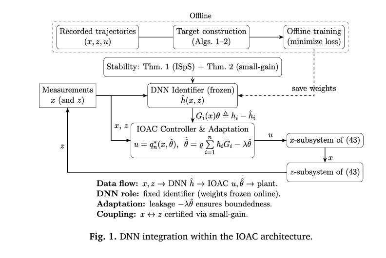
Enter a groundbreaking solution: deep neural network (DNN)-augmented inverse optimal adaptive control (IOAC). This innovative framework, recently proposed in a peer-reviewed study published in Neurocomputing, merges the universal approximation power of deep learning with rigorous stability guarantees from stochastic control theory. By integrating DNN-based identifiers, inverse optimal control, and the small-gain theorem, this approach ensures input-to-state practical stability in probability (SISpS)—even in the presence of significant uncertainties.

In this article, we unpack the core ideas behind this method, explain its mathematical foundations in accessible terms, and illustrate its real-world impact through a detailed case study on an automobile suspension system. Whether you’re a control engineer, a machine learning practitioner, or a researcher in applied mathematics, you’ll gain actionable insights into how AI and control theory can converge to solve some of today’s toughest stability challenges.

Why Traditional Control Fails in Stochastic Interconnected Systems

Interconnected systems consist of multiple subsystems whose states influence one another—often bidirectionally. Unlike cascade systems (where influence flows in one direction), interconnected systems create feedback loops of dependency, making stability analysis far more complex.

When stochastic noise—such as Brownian motion—is added to the mix, the problem intensifies. The system dynamics become:

\[ dx(t) = f(x)\,dt + g(x)\,u\,dt + h(x)\,dw \]

where:

x ∈ Rⁿ is the state,
u ∈ R^m is the control input,
w is a standard Wiener process (modeling random disturbances),
f , g , and h are nonlinear functions, possibly unknown.

Key challenges include:

Unmodeled dynamics: Parts of the system (e.g., hidden states z ) are not directly observable.
Unknown nonlinearities: Functions like f (x,z) cannot be precisely characterized.
Mutual coupling: Subsystems affect each other, risking instability propagation.

Conventional model-based controllers require exact knowledge of these functions—something rarely available in practice.

💡 Takeaway: Without a robust strategy to handle uncertainty and interconnection, even small disturbances can cause catastrophic failure in safety-critical systems like aircraft or autonomous vehicles.

The Core Innovation: DNN-Augmented Inverse Optimal Adaptive Control

The proposed IOAC framework tackles these issues through a three-pronged strategy:

1. Deep Neural Networks for Real-Time Uncertainty Estimation

Each subsystem is equipped with a DNN-based identifier trained to approximate unknown nonlinearities such as h^i(xi,z)≈hi(xi,z) . The network:

Uses two hidden layers with 64 neurons each,
Employs Exponential Linear Unit (ELU) activations for smooth gradients,
Is trained offline on input-output pairs derived from system trajectories,
Operates online as a static map during control execution.

This allows the controller to compensate for unmodeled effects in real time, without requiring explicit analytical models.

2. Inverse Optimal Control Without Solving HJB Equations

Traditional optimal control relies on solving the Hamilton–Jacobi–Bellman (HJB) equation—a task that becomes intractable for high-dimensional stochastic systems.

Instead, inverse optimal control (IOC) flips the script:

First, design a stabilizing controller using Lyapunov-based methods.
Then, identify the cost functional that this controller implicitly minimizes.

This avoids the computational nightmare of HJB while still guaranteeing performance optimality.

The minimized cost functional takes the form:

\[ J(\upsilon) = \sup_{z \in \Omega_z} \Bigg\{ \lim_{t \to \infty} \Big[ \pi(x, \hat{\theta}) + \iota \| \theta – \hat{\theta}^{(t)} \|^2 + \int_{0}^{t} \big( \rho(x, \hat{\theta}) + \rho_{\theta}(\hat{\theta}) + \upsilon^{T} R^{2}(x, \hat{\theta}) \upsilon – \gamma^{2} \| z \| \big) ds \Big] \Bigg\} \]

This formulation explicitly accounts for parameter estimation error and unmodeled dynamics, making it uniquely suited for adaptive settings.

3. Small-Gain Theorem for Stability Certification

To manage bidirectional coupling between subsystems, the authors employ the stochastic small-gain theorem. This ensures that the gain product of interconnected subsystems satisfies:

\[ \chi_{1}(s) \circ \chi_{2}(s) \le s, \quad \forall\, s \ge s_{0} \]

where χ1,χ2 are gain functions derived from Lyapunov bounds. When this condition holds, the entire interconnected system is stochastically input-to-state practically stable (SISpS)—meaning all states remain bounded and converge to a small neighborhood around the origin.

✅ Result: The closed-loop system remains uniformly bounded, and states converge near zero despite noise and uncertainty.

Step-by-Step Controller Design: From Theory to Implementation

The control design proceeds in stages, combining backstepping, adaptive laws, and DNN estimation.

System Structure

Consider an n -dimensional stochastic system:

\[ \begin{cases} dz = f_0(z, x)\,dt + h_0(z, x)\,d\omega, \\[6pt] dx_i = x_{i+1}\,dt + h_i(x_i, z)\,dt + \xi_i(x_i, z)\,d\omega, & i = 1, \ldots, n-1, \\[6pt] dx_n = \upsilon\,dt \end{cases} \]

Here, z represents unmodeled dynamics, and hi are unknown nonlinearities.

DNN Estimation Pipeline

STEP	DESCRIPTION
Data Collection	Simulate system trajectories; computeh_i ≈ (dx_i − x_i+1dt)/dt
Training	Use PyTorch with Adam optimizer (lr = 1e⁻⁵), MSE loss, 2000 epochs
Deployment	Fixed DNN used online to predict h_i (x_i, z) in real time

Adaptive Control Law

The final control law is:

\[ \upsilon = q_n^{*}(x, \hat{\theta}) = -\beta R(x, \hat{\theta}) – \frac{1}{\hbar n}, \quad \beta \ge 2 \]

with adaptive parameter update:

\[ \dot{\theta} = \rho \sum_{i=1}^{n} \hbar_i \, \bar{G}_i – \lambda \hat{\theta}, \quad \lambda, \rho > 0 \]

where:

\[ \hbar_i = x_i – q_{i-1}(x_1, \ldots, x_{i-1}, \hat{\theta}) \] are the **error coordinates**, \[ R(x, \hat{\theta}) > 0 \] ensures **control effort penalization**, and \[ \bar{G}_i \] captures the **effect of parameter uncertainty**.

This design guarantees Lyapunov stability and inverse optimality simultaneously.

Real-World Validation: Automobile Suspension System

To demonstrate practicality, the authors apply their method to a stochastic automobile suspension system:

\[ \begin{cases} dz = (-2z + 0.25x_1)\,dt + 0.5x_1\,d\omega, \\[6pt] dx_1 = (x_2 + h(x_1, z))\,dt + 0.5x_1 z\,d\omega, \\[6pt] dx_2 = \upsilon\,dt \end{cases} \]

with unknown nonlinearity h(x₁,z)=0.5x₁²z .

Results Summary

METRIC	OUTCOME
State Boundedness	z (t), x₁ (t), x₂ (t) remain uniformly bounded
Parameter Convergence	θ^{^}(t) converges to true value
Control Signal	Smooth, physically realizableυ (t)
Stability	Small-gain condition satisfied; SISpS achieved

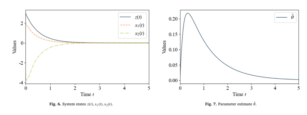
📊 Insight: Even with significant stochastic disturbance (dω ), the system exhibits excellent transient performance and robustness to uncertainty—critical for ride comfort and vehicle safety.

Advantages Over Existing Methods

FEATURE	Traditional Adaptive Control	DNN-Augmented IOAC (This Work)
Model Dependency	Requires known structure	Handlescompletely unknownnonlinearities
Optimality	Rarely guaranteed	Inverse optimalby construction
Scalability	Limited to low dimensions	Scales viamodular DNNs per subsystem
Stability Proof	Often heuristic	RigorousSISpS via small-gain theorem
Real-Time Adaptation	Slow parameter tuning	Fast DNN inference + adaptive laws

This hybrid approach bridges the gap between data-driven learning and model-based guarantees—a rare and powerful combination.

Future Directions and Practical Implications

The authors outline several promising extensions:

Multi-agent systems with uncertain communication topologies,
High-dimensional networks using decentralized DNNs,
Embedded deployment via model pruning and quantization,
Safety-critical applications with state/input constraints,
Probabilistic small-gain conditions for more realistic uncertainty models.

For industries like automotive, aerospace, and robotics, this means more reliable, adaptive, and optimal control without sacrificing theoretical safety assurances.

Conclusion: A New Paradigm for Robust Intelligent Control

The fusion of deep learning, inverse optimal control, and stochastic small-gain theory represents a major leap forward in managing complex, uncertain systems. By replacing intractable PDEs with trainable neural estimators and grounding the design in rigorous stability theory, this approach delivers both performance and trustworthiness.

🚀 Ready to explore this further?
If you’re working on autonomous systems, industrial automation, or stochastic control, consider implementing a DNN-augmented IOAC framework in your next project. Share your results, questions, or adaptations in the comments below—we’d love to hear how you’re pushing the boundaries of intelligent control!

Have you used neural networks in control systems? What challenges did you face? Join the conversation and help shape the future of adaptive robotics and AI-driven engineering.

Download Paper Here.

Below is the the end-to-end implementation of the paper code. It builds and trains the neural network, then uses it as a component within the adaptive control loop to stabilize the stochastic system described in the paper.

import numpy as np
import torch
import torch.nn as nn
import torch.optim as optim
from torch.utils.data import TensorDataset, DataLoader
import matplotlib.pyplot as plt
import time

# --- 1. DNN Definition (Based on Algorithm 3) ---
# The DNN is used to approximate the unknown function h(x1, z)
class DNN(nn.Module):
    def __init__(self):
        """
        Defines the DNN architecture as described in the paper:
        Input (x1, z) -> 64 (ELU) -> 64 (ELU) -> Output (h_hat)
        """
        super(DNN, self).__init__()
        self.layer_1 = nn.Linear(2, 64)
        self.layer_2 = nn.Linear(64, 64)
        self.layer_out = nn.Linear(64, 1)
        self.elu = nn.ELU()

    def forward(self, x):
        """Forward pass through the network."""
        x = self.elu(self.layer_1(x))
        x = self.elu(self.layer_2(x))
        x = self.layer_out(x)
        return x

# --- 2. Data Generation for Offline Training ---
def get_training_data(num_samples=5000):
    """
    Generates synthetic data for training the DNN.
    The "unknown" function to learn is h(x1, z) = 0.5 * x1^2 * z (from Sec 5).
    """
    # Generate random inputs within a reasonable range
    x1_data = np.random.uniform(-3, 3, (num_samples, 1))
    z_data = np.random.uniform(-4, 4, (num_samples, 1))
    
    # Calculate the "true" output h(x1, z)
    h_data = 0.5 * (x1_data**2) * z_data
    
    # Create the input features [x1, z]
    X_data = np.hstack((x1_data, z_data))
    
    # Convert to PyTorch tensors
    X_tensor = torch.tensor(X_data, dtype=torch.float32)
    y_tensor = torch.tensor(h_data, dtype=torch.float32)
    
    return X_tensor, y_tensor

# --- 3. DNN Training Function (Based on Algorithm 1) ---
def train_dnn(model, X_train, y_train):
    """
    Trains the DNN model based on the parameters in Algorithm 1.
    """
    # Parameters from the paper
    epochs = 2000
    batch_size = 64
    learning_rate = 1e-5
    
    # Loss and Optimizer
    criterion = nn.MSELoss()
    optimizer = optim.Adam(model.parameters(), lr=learning_rate)
    
    # Create DataLoader
    dataset = TensorDataset(X_train, y_train)
    loader = DataLoader(dataset, batch_size=batch_size, shuffle=True)
    
    start_time = time.time()
    for epoch in range(epochs):
        for X_batch, y_batch in loader:
            # Forward pass
            y_pred = model(X_batch)
            loss = criterion(y_pred, y_batch)
            
            # Backward pass and optimization
            optimizer.zero_grad()
            loss.backward()
            optimizer.step()
            
        if (epoch + 1) % 200 == 0:
            print(f'Epoch [{epoch+1}/{epochs}], Loss: {loss.item():.6f}')
            
    end_time = time.time()
    print(f"Training finished in {end_time - start_time:.2f}s")
    
    # Set model to evaluation mode (freezes weights)
    model.eval()

# --- 4. Simulation of the Controlled System ---
class SuspensionSystemSimulator:
    """
    Implements the full simulation of the stochastic automobile suspension system
    (Eq. 51) with the DNN-augmented adaptive controller (Sec 4.2 & 5).
    """
    def __init__(self, dnn_model):
        self.dnn_model = dnn_model
        
        # --- Simulation Parameters ---
        self.T = 5.0  # Total time (from graphs)
        self.dt = 0.01 # Time step (from Alg 1)
        self.num_steps = int(self.T / self.dt)
        self.t = np.linspace(0, self.T, self.num_steps + 1)
        
        # --- Controller Parameters (from Sec 5) ---
        self.c1 = 1.0
        self.c2 = 5.0
        self.rho = 2.0   # For adaptation law (Eq 50)
        self.lambd = 0.5 # For adaptation law (Eq 50, "o=0.5" in text)
        # Note: beta and R from Eq. 50 are for IOAC *analysis*.
        # The controller implementation is a standard adaptive backstepping design.
        # We use c2 as the final gain.
        
        # --- Initial States (from Sec 5 and Fig 6) ---
        self.z = 3.0
        self.x1 = 2.0
        self.x2 = -4.0
        self.theta_hat = 0.0 # Parameter estimate (Fig 7)
        
        # --- Data Loggers ---
        self.z_history = [self.z]
        self.x1_history = [self.x1]
        self.x2_history = [self.x2]
        self.theta_hat_history = [self.theta_hat]
        self.u_history = [0.0]

    def run_simulation(self):
        """
        Runs the full simulation using Euler-Maruyama method.
        """
        for i in range(self.num_steps):
            # --- Generate Stochastic Wiener process increments ---
            dw0 = np.random.normal(0.0, 1.0) * np.sqrt(self.dt)
            dw1 = np.random.normal(0.0, 1.0) * np.sqrt(self.dt)
            
            # --- 4.1. Controller and Adaptation Law ---
            
            # Get DNN's estimate of the unknown function h(x1, z)
            # This is h_hat in the paper.
            with torch.no_grad():
                input_tensor = torch.tensor([[self.x1, self.z]], dtype=torch.float32)
                h_hat_1 = self.dnn_model(input_tensor).item()
            
            # Backstepping Step 1:
            h1 = self.x1 # h1 = x1 - q0, where q0 = 0
            
            # G_bar_1 = G1 (from paper Sec 5: G1 = 0.5*x1^2)
            G_bar_1 = 0.5 * self.x1**2
            
            # Virtual control q1 (simplified from Eq 46)
            # q1 = -c1*h1 - h_hat_1 - G_bar_1 * theta_hat
            q1 = -self.c1 * h1 - h_hat_1 - G_bar_1 * self.theta_hat
            
            # Backstepping Step 2:
            h2 = self.x2 - q1
            
            # Control Law u (from standard backstepping)
            # This is the realizable controller that the IOAC framework analyzes.
            # u = -h1 - c2*h2
            u = -h1 - self.c2 * h2
            
            # Adaptation Law (from Eq 50)
            # hat(theta)_dot = rho * sum(h_i * G_bar_i) - lambda * hat(theta)
            # G_bar_2 = 0 (since G2 = 0 and we simplify derivative terms)
            # This matches the paper's implication that the adaptation law
            # is driven by the error in the first subsystem.
            d_theta_hat = (self.rho * (h1 * G_bar_1) - self.lambd * self.theta_hat) * self.dt
            
            
            # --- 4.2. System Dynamics (Eq. 51) ---
            
            # This is the "true" function, which the controller does *not* know.
            h_true = 0.5 * (self.x1**2) * self.z
            
            # Euler-Maruyama update
            dz = (-2.0 * self.z + 0.25 * self.x1) * self.dt + (0.5 * self.x1) * dw0
            dx1 = (self.x2 + h_true) * self.dt + (0.5 * self.x1 * self.z) * dw1
            dx2 = u * self.dt
            
            # --- 4.3. Update States ---
            self.z += dz
            self.x1 += dx1
            self.x2 += dx2
            self.theta_hat += d_theta_hat
            
            # --- 4.4. Log Data ---
            self.z_history.append(self.z)
            self.x1_history.append(self.x1)
            self.x2_history.append(self.x2)
            self.theta_hat_history.append(self.theta_hat)
            self.u_history.append(u)

    def plot_results(self):
        """
        Plots the simulation results, replicating Figs 6, 7, and 8.
        """
        plt.style.use('seaborn-v0_8-whitegrid')
        fig, (ax1, ax2, ax3) = plt.subplots(3, 1, figsize=(10, 15))
        fig.suptitle('DNN-IOAC Suspension System Simulation Results', fontsize=16)
        
        # Plot 1: System States (Fig 6)
        ax1.plot(self.t, self.z_history, label='z(t) (unmodeled dynamics)')
        ax1.plot(self.t, self.x1_history, label='x1(t) (suspension disp.)', linestyle='--')
        ax1.plot(self.t, self.x2_history, label='x2(t) (suspension vel.)', linestyle='-.')
        ax1.set_title('System States vs. Time (Fig 6)')
        ax1.set_xlabel('Time (t)')
        ax1.set_ylabel('Values')
        ax1.legend()
        ax1.set_ylim(-4.5, 3.5) # Match paper's scale
        
        # Plot 2: Parameter Estimate (Fig 7)
        ax2.plot(self.t, self.theta_hat_history, label='$\hat{\\theta}(t)$', color='k')
        ax2.set_title('Parameter Estimate vs. Time (Fig 7)')
        ax2.set_xlabel('Time (t)')
        ax2.set_ylabel('Values')
        ax2.legend()
        
        # Plot 3: Control Input (Fig 8)
        ax3.plot(self.t, self.u_history, label='u(t) (control input)', color='k')
        ax3.set_title('Inverse Optimal Controller vs. Time (Fig 8)')
        ax3.set_xlabel('Time (t)')
        ax3.set_ylabel('Values')
        ax3.legend()
        
        plt.tight_layout(rect=[0, 0.03, 1, 0.96])
        plt.show()

# --- 5. Main Execution ---
if __name__ == "__main__":
    
    # --- Step 1: Generate Data ---
    print("Generating training data for DNN...")
    X_train, y_train = get_training_data(num_samples=10000)
    
    # --- Step 2: Define and Train DNN ---
    print("Initializing DNN...")
    dnn_identifier = DNN()
    
    print("Training DNN (this may take a minute)...")
    # Set to true to retrain, false to load a saved model
    TRAIN_MODEL = True 
    
    if TRAIN_MODEL:
        train_dnn(dnn_identifier, X_train, y_train)
        # Save the trained model
        torch.save(dnn_identifier.state_dict(), 'dnn_model.pth')
        print("Model trained and saved as 'dnn_model.pth'.")
    else:
        try:
            dnn_identifier.load_state_dict(torch.load('dnn_model.pth'))
            dnn_identifier.eval()
            print("Loaded pre-trained model 'dnn_model.pth'.")
        except FileNotFoundError:
            print("No pre-trained model found. Training new model...")
            train_dnn(dnn_identifier, X_train, y_train)
            torch.save(dnn_identifier.state_dict(), 'dnn_model.pth')
            print("Model trained and saved as 'dnn_model.pth'.")

    # --- Step 3: Run Simulation ---
    print("\nRunning stochastic simulation with DNN-IOAC controller...")
    simulator = SuspensionSystemSimulator(dnn_identifier)
    simulator.run_simulation()
    print("Simulation complete.")
    
    # --- Step 4: Plot Results ---
    print("Plotting results...")
    simulator.plot_results()

Related posts, You May like to read