
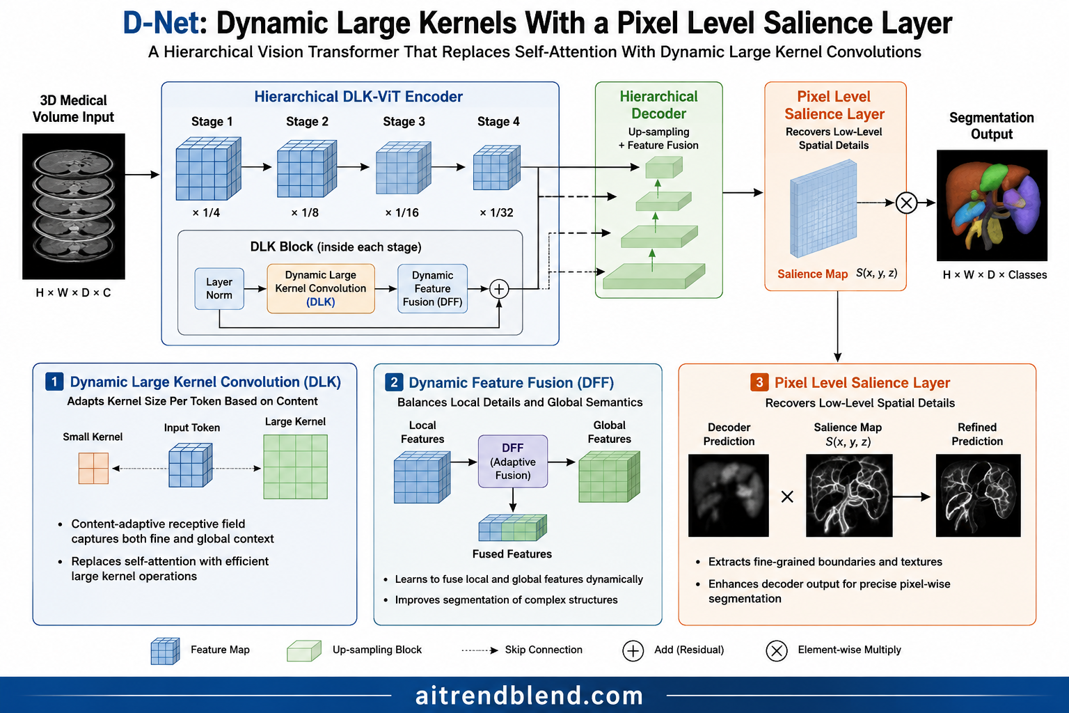
- D-Net replaces the self attention block inside a hierarchical vision transformer with a Dynamic Large Kernel module, which stacks two large depthwise convolutions and then dynamically decides which of them to trust at each location.
- A companion Dynamic Feature Fusion module replaces the usual concatenation of encoder and decoder features with a channel and spatial aware fusion step that the ablation study shows outperforms a well known alternative called Attentional Feature Fusion.
- A Salience layer processes the input image at its original resolution, bypassing the early downsampling that hierarchical vision transformers normally apply, specifically to recover fine detail that gets lost before the network ever sees it.
- Across three very different segmentation tasks, abdominal organs in CT, brain tumor subregions in MRI, and hepatic vessels and tumors in CT, D-Net reported the highest mean Dice score of every method tested while using fewer parameters and less compute than most of its competitors.
- An external zero shot test on a separate spleen dataset found D-Net kept the smallest performance gap between its internal and external results among the top performing methods, a proxy for how well the model generalizes beyond its training distribution.
- The paper’s own failure case analysis found that segmentation errors clustered on the same specific cases regardless of which architecture was used, including one case the authors suspect has a mislabeled ground truth annotation rather than a genuinely hard image.
Why hierarchical transformers quietly give up on fine detail
Segmenting organs and lesions in medical images is one of those tasks that sounds simple until you have to automate it at scale. Manual segmentation by a radiologist is accurate but slow and inconsistent from one reader to the next, which is exactly the kind of problem deep learning has spent the last decade trying to solve. Vision transformers pushed that effort forward by giving networks a genuinely global view of an image through self attention, letting a model relate a pixel in one corner of a scan to a pixel far away without needing to pass information through a long chain of local convolutions first. The catch is that self attention’s compute and memory cost scales quadratically with how many pixels it looks at, which turns a full resolution 3D CT or MRI volume into a serious computational problem almost immediately.
Hierarchical vision transformers exist specifically to defuse that problem, approximating self attention with something closer to linear cost so it can actually run on 3D data during both training and inference. The way they typically do this is by shrinking the image early, using a convolutional stem with a stride of 4 so that everything downstream operates on a feature map at a quarter of the original height and width. For image classification that tradeoff barely registers, because classification only needs to answer one question about the whole image. Segmentation is a fundamentally different kind of task. It has to label every single voxel correctly, and that early downsampling throws away exactly the fine grained spatial detail that boundary precision depends on. The paper argues this specific limitation has been quietly present in a lot of prior work without being clearly named as its own problem, even though a handful of methods, ordinary convolutional networks such as U-Net among them, sidestep it by processing the full resolution image directly in their first layers.
Convolutional networks have the opposite problem. Their convolutional kernels are inherently local, which makes them excellent at picking up fine detail but genuinely limited at modeling long range dependencies between features that are far apart in the image. Large kernel convolutions were introduced specifically to close that gap by widening a CNN’s receptive field without resorting to self attention. But the paper points out that most existing large kernel networks still use one fixed kernel size for everything, which limits their ability to adapt to organs that vary enormously in shape and size from one patient to the next, and they generally lack any mechanism for letting local and global information talk to each other during feature extraction.
The paper’s framing is unusually specific about where existing designs actually fail. It is not that hierarchical transformers are bad at segmentation in general, it is that their standard convolutional stem discards fine spatial detail before the rest of the network gets a chance to use it, and that discarding is easy to overlook because it does not show up as an obvious architectural flaw, only as a ceiling on boundary accuracy that quietly caps performance.
Three components, each built to answer one specific gap
D-Net is built around three named components, and the paper is explicit that each one targets a distinct failure mode rather than being a generic accuracy booster bolted on for its own sake.
The Dynamic Large Kernel module
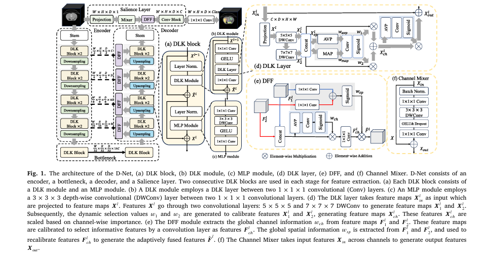
The Dynamic Large Kernel layer takes an input feature map, projects it down to half its channel count through a small convolution to keep the computation manageable, and then runs it through two depthwise convolutions in sequence rather than in parallel. The first uses a 5 by 5 by 5 kernel with no dilation. The second uses a 7 by 7 by 7 kernel with a dilation rate of 3, which effectively behaves like a much bigger kernel while only paying the computational cost of a 7 by 7 by 7 one. Chaining these two convolutions rather than running them side by side, the way Atrous Spatial Pyramid Pooling famously does, lets the effective receptive field grow recursively, and the paper works out that the combined effective receptive field of this two step cascade is equivalent to a single 23 by 23 by 23 convolution.
Working through that formula with the paper’s own numbers is genuinely clarifying. The first 5 by 5 by 5 kernel gives a starting receptive field of 5. The second layer has a stride of 1 and, because of its dilation rate of 3, an effective kernel size of 19 rather than 7. Plugging those values in gives 5 plus 19 minus 1 times 1, which comes out to 23. That is a large receptive field bought at the cost of two comparatively small convolutions rather than one genuinely enormous one, which is the efficiency argument for cascading kernels instead of just using a bigger single kernel.
Having two feature maps from two differently shaped kernels is only useful if the network can decide which one to trust at any given location, and that is where the dynamic part of the module comes in. The two feature maps are concatenated back to the original channel count, then average pooled and max pooled along the channel dimension to summarize their global spatial relationships, passed through a convolution that lets those two pooled summaries interact, and squeezed through a sigmoid to produce two selection weight maps. Those weights recombine the two kernel outputs into a single calibrated feature map, which then goes through a second, channel focused calibration step using average pooling and another sigmoid gate before a residual connection closes the block. The whole module gets wrapped, along with a small MLP block, into what the paper calls a DLK block, which is dropped directly into a hierarchical ViT architecture in place of its usual multi head self attention layer.
The Dynamic Feature Fusion module
Skip connections are a defining feature of U shaped segmentation networks, but the standard way of using them, concatenating encoder features with decoder features, does not distinguish between features that actually matter at a given spatial location and features that are mostly noise. The Dynamic Feature Fusion module replaces that plain concatenation with a two stage gating process. First, the two feature maps are concatenated and a global channel importance weight is computed through average pooling, a convolution, and a sigmoid activation, which is used to compress the fused feature map back down to its original channel count while preferentially keeping the more informative channels rather than just averaging everything together. Second, a separate spatial importance weight is computed directly from the two original feature maps before fusion, and that weight recalibrates the channel fused output to emphasize the spatial regions that matter most. The result replaces every skip connection in the network with a fusion step that is explicitly conditioned on global context rather than a fixed operation applied uniformly everywhere.
The Salience layer
This is the piece that most directly answers the early downsampling problem described above. Rather than accepting that fine spatial detail is simply gone once the convolutional stem shrinks the image, the Salience layer processes the input volume at its original, unshrunk resolution in a separate path. A small convolutional block first projects the number of channels to match the rest of the network without touching the spatial resolution at all. Then a component the authors call the Channel Mixer, built from batch normalization, a channel expanding convolution, a depthwise convolution, a GELU activation, dropout, and a channel compressing convolution wrapped in a residual connection, learns global relationships between channels while still operating at full resolution. The features this layer extracts are fused with the upsampled features coming out of the decoder using the same Dynamic Feature Fusion module described above, giving the network one path that has never lost fine spatial detail and one path that has learned rich hierarchical context, merged together rather than forced to choose between them.
How the pieces assemble into D-Net
D-Net follows a familiar overall shape for anyone who has looked at a medical segmentation network before, a U shaped encoder, bottleneck, and decoder, with the Salience layer bolted on as an additional path rather than replacing any part of that core structure. The encoder starts with a 7 by 7 by 7 convolutional stem with a stride of 2, which is a gentler initial downsampling than the stride of 4 typically used in classification style hierarchical ViTs, immediately reflecting the paper’s stated priority of preserving more spatial detail from the start. Each stage of the encoder runs two consecutive DLK blocks, and downsampling between stages is handled by an ordinary 3 by 3 by 3 convolution with a stride of 2, which halves the spatial resolution while doubling the channel count at each step. The bottleneck runs two more DLK blocks at the network’s lowest resolution and highest channel count. The decoder mirrors the encoder in reverse, using transposed convolutions to upsample and Dynamic Feature Fusion modules in place of ordinary skip connections at every stage, before the Salience layer’s full resolution features get folded in near the very end and a final 1 by 1 by 1 convolution produces the voxel level segmentation output.
Testing across three genuinely different segmentation problems
The paper does not lean on a single benchmark to make its case. It evaluates D-Net on three tasks that differ in imaging modality, number of target structures, and the underlying clinical questions involved, which is a reasonable way to test whether an architectural idea generalizes or was just tuned to one dataset’s quirks. The comparison set is broad too, spanning pure convolutional networks such as VNet, nnU-Net, and Att U-Net, transformer based methods such as nnFormer and SegFormer, hybrid CNN and ViT designs such as TransBTS, UNETR, Swin UNETR, and VSmTrans, and other large kernel hybrid designs such as 3D UX Net and MedNext.
| Task | D-Net mean Dice | Best competing method | Competing Dice |
|---|---|---|---|
| AMOS abdominal organs, 15 structures | 89.67 | Att U-Net | 87.56 |
| MSD brain tumor, 3 subregions | 74.42 | VSmTrans | 74.00 |
| MSD hepatic vessel and tumor | 67.63 | MedNext | 66.16 |
Mean Dice score across all tasks, with all differences between D-Net and the compared methods reported as statistically significant at p below 0.01 using the Wilcoxon signed rank test.
The AMOS abdominal result is the largest margin of the three, and the paper reports D-Net leading on organ specific Dice scores as well, including a 97.60 score on the spleen, 97.06 on the right kidney, and notably strong performance on some of the harder structures in the set, the gall bladder at 85.01, the duodenum at 82.73, and both adrenal glands, which are small, variably shaped structures that tend to be where segmentation networks struggle most. The brain tumor and hepatic vessel results are tighter contests, which makes sense given how competitive the SOTA field already is on those specific tasks, but D-Net still comes out ahead on every reported metric in both.
| Method | Params in millions | FLOPs in billions | AMOS mean Dice |
|---|---|---|---|
| UNETR | 92.78 | 82.73 | 74.73 |
| nnFormer | 149.33 | 284.28 | 81.65 |
| 3D UX Net | 53.01 | 632.33 | 85.52 |
| VSmTrans | 50.39 | 358.21 | 87.08 |
| MedNext | 11.65 | 178.05 | 84.91 |
| D-Net | 39.28 | 200.13 | 89.67 |
Computational complexity measured on input patches of 96 cubed voxels. D-Net beats the highest scoring competitor, VSmTrans, while using 22 percent fewer parameters and 45 percent fewer FLOPs.
MedNext is the one method in this comparison with fewer parameters than D-Net, and SegFormer is dramatically smaller still, using roughly 90 percent fewer parameters and 98 percent fewer FLOPs than D-Net. Neither one matches D-Net’s accuracy, which is the tradeoff the paper is arguing for directly, that a moderate increase in computational cost over the very smallest architectures buys a meaningfully large jump in segmentation quality, while still coming in well under the cost of most of the larger transformer heavy alternatives.
What happens when the model sees a dataset it was never trained on
Benchmark accuracy on data the model was trained and tested on tells you one thing. Generalization to genuinely unseen data tells you something arguably more important for any real deployment. The paper tests this directly by taking D-Net and every competing method, all trained only on the AMOS abdominal dataset, and applying them without any additional training to a separate MSD spleen dataset collected from a different patient population.
| Method | AMOS spleen, internal | MSD spleen, external zero shot | Generalization gap |
|---|---|---|---|
| VNet | 95.06 | 90.43 | 4.63 |
| nnU-Net | 96.37 | 91.92 | 4.45 |
| VSmTrans | 95.90 | 89.72 | 6.18 |
| SegFormer | 92.07 | 88.66 | 3.41 |
| D-Net | 97.60 | 94.12 | 3.48 |
D-Net posts the highest score on the external dataset by a margin of roughly 1.5 to 8 points over other methods, and its generalization gap is close to the smallest recorded, only slightly behind SegFormer, a far smaller model whose accuracy trails considerably on both the internal and external tasks.
A small generalization gap paired with a high absolute score is a meaningfully different result than a small gap paired with a mediocre score, and this is where D-Net’s combination stands out. It is not just accurate on data resembling its training set, it also degrades less than most competitors when the input distribution shifts, which is a more demanding and arguably more clinically relevant test than the standard held out split most papers report.
Reading the ablation study as a checklist rather than a footnote
An ablation study is where a paper either earns its architectural claims or exposes that some of its components were not doing much. D-Net’s ablations are unusually thorough, running four separate studies against the AMOS dataset.
The first isolates the Dynamic Large Kernel design itself. Swapping a plain 5 by 5 by 5 convolution for the full 23 by 23 by 23 effective receptive field, without yet adding the dynamic selection mechanism, improved mean Dice by about 1 point in a hybrid convolution and ViT backbone and about 0.6 points in the full D-Net backbone. Adding the dynamic selection mechanism on top of that larger receptive field added a further 1 to 1.5 points. Both pieces of the design, the larger cascaded receptive field and the dynamic recombination of what it sees, are independently earning their place, and the cost of adding them is modest, roughly an 8 percent increase in parameters and either an 8 percent or a 2 percent increase in FLOPs depending on the backbone.
The second isolates Dynamic Feature Fusion. Adding it to four different backbones, a pure convolutional nnU-Net, a hybrid convolution and ViT backbone, a DLK equipped hybrid, and full D-Net, improved mean Dice by 1 to 2 points in every case, generally for a negligible increase in parameters and FLOPs. The paper also runs a direct comparison against Attentional Feature Fusion, an established alternative fusion module from the broader computer vision literature, and finds Dynamic Feature Fusion outperforms it by roughly 2 to 4 Dice points across the same three backbones, which is a genuinely useful data point for anyone deciding between fusion strategies for their own segmentation network.
The third isolates the Salience layer, comparing no salience path at all against three alternative designs for what should sit inside it, an ordinary convolutional block, a block built from stacked DLK modules, and the Channel Mixer the paper ultimately settled on. Adding any version of the Salience layer improved Dice by roughly 1 to 3 points over having none at all. Among the three internal design choices, the Channel Mixer edged out the convolutional block by a small margin, 89.67 against 89.34, while using about 15 percent fewer FLOPs, making it the more efficient choice for essentially the same accuracy.
The fourth ablation takes a different approach entirely, building a separate hybrid network called DLK-NETR that swaps the DLK module into the encoder of an existing family of architectures, UNETR, Swin UNETR, 3D UX Net, and VSmTrans all share this same hybrid transformer encoder and convolutional decoder layout, differing mainly in what module sits inside the encoder. Slotting DLK into that same position beat every one of those established designs on all three of the paper’s segmentation tasks, while using fewer parameters than all of them, which is a fairly direct way of isolating how much of D-Net’s advantage traces back to the DLK module specifically rather than to some other part of the overall architecture.
Extracting local features enhances the precision of segmenting small organs and improves accuracy in boundary regions, and global information helps a network disambiguate what those local features actually mean. Paraphrased from Yang, Qiu, Zhang, Marcus and Sotiras, Biomedical Signal Processing and Control, 2026
Where the model still fails, and what that failure pattern suggests
The paper’s failure case analysis is more interesting than the usual limitations paragraph tacked onto the end of a results section, because it does not stop at cataloguing D-Net’s own weak points. It looks at every method’s worst performing cases across all three datasets and finds a striking pattern, the same specific cases tend to be hard for every architecture tested, regardless of whether that architecture is a pure convolutional network, a hybrid convolution and transformer design, or a large kernel hybrid like D-Net itself. That consistency across genuinely different architectural families is the authors’ basis for suggesting the difficulty is not primarily an architectural shortcoming but something closer to an intrinsic property of specific anatomical or pathological cases, images that are simply harder to segment no matter what tool is pointed at them.
One case in particular stands out. Every method tested, D-Net included, scored close to zero Dice on the same case from the hepatic vessel and tumor dataset. After examining that case directly against its ground truth annotation, the authors concluded the most likely explanation is a misalignment between the raw scan and its corresponding label, essentially a data quality problem in the benchmark rather than a genuine segmentation failure on any model’s part. That is a useful reminder for how to read failure case tables in any segmentation paper, a universally low score across every competing method is at least as likely to be pointing at the dataset as at any particular network.
What this means beyond the three tasks tested here
The specific numbers in this paper are tied to abdominal organs, brain tumor subregions, and hepatic vessels and tumors, but the underlying design argument is broader than any single task. Any volumetric segmentation problem that needs both a wide receptive field to understand where an anatomical structure sits relative to its neighbors and fine local detail to trace its actual boundary is a reasonable candidate for the same combination of ideas, cascaded dynamic large kernels for scalable local context, a fusion mechanism that weighs features rather than just concatenating them, and a dedicated path that never lets the original image resolution get thrown away before the network sees it. Lung nodules, cardiac substructures, and spinal anatomy all share that same basic tension between needing global anatomical context and needing pixel accurate boundaries, which makes them plausible directions for this general approach even though the paper itself does not test them.
Conclusion
D-Net’s central argument is not that transformers were the wrong idea for medical image segmentation. It is that the specific way hierarchical vision transformers achieve their computational efficiency, by aggressively downsampling the input before the network really gets to work, quietly costs segmentation networks the fine spatial detail that pixel level tasks depend on, and that cost has mostly gone unaddressed as its own distinct problem rather than as a side effect of other design choices. The paper’s answer is not to abandon the hierarchical transformer scaffold but to replace its most computationally expensive component with something built specifically for local context, and to add a dedicated path that keeps the original resolution image in play the whole time rather than only in the network’s very first layer.
The results back that argument up with more than a single headline number. D-Net topped every comparison method across three genuinely different segmentation tasks, kept a smaller generalization gap than most competitors on a held out external dataset, and did all of this with parameter and compute costs that sit comfortably in the middle of the field rather than at either extreme. The ablation studies trace the improvement back to each individual component rather than leaving readers to take the overall result on faith, and the direct head to head test against Attentional Feature Fusion and against four established hybrid architectures using the DLK-NETR variant both point the credit specifically at the Dynamic Large Kernel and Dynamic Feature Fusion designs rather than at some incidental part of the network.
The honest caveat sits in what the failure case analysis reveals. Certain cases are hard for every architecture tested, which is a useful signal that some of the remaining performance ceiling in this space may have more to do with data quality and inherent case difficulty than with any specific network design, D-Net’s included. That is a genuinely useful finding for the field to sit with rather than a weakness unique to this paper, since it suggests future gains might come as much from better annotated benchmarks as from further architectural refinement.
What D-Net demonstrates most clearly is narrower and more concrete than a claim to have solved medical image segmentation outright. It shows that treating the loss of fine spatial detail in hierarchical transformers as a specific, nameable problem, rather than an unavoidable side effect of efficient attention, opens room for a design that keeps most of the benefits transformers brought to the field while directly repairing one of their clearest weaknesses for pixel level tasks.
As with any research benchmark result, translating this from a strong showing on three public datasets into something used in an actual clinical pipeline would require substantially more validation, regulatory review, and testing across the kind of imaging variability real hospitals produce, none of which this paper claims to have done and none of which this article should be read as implying.
A simplified PyTorch implementation of the D-Net components
The paper’s own code is available from the authors directly and is the version to use for any real research work. The implementation below is a compact, from scratch reconstruction of the three named components described in the Method section, the Dynamic Large Kernel layer and block, the Dynamic Feature Fusion module, and the Salience layer with its Channel Mixer, wired together into a small illustrative encoder and decoder with a runnable smoke test on synthetic volumetric data.
# ==============================================================================
# D-Net, a simplified reconstruction of the core method
# Paper: https://doi.org/10.1016/j.bspc.2025.108837
# Authors: Jin Yang, Peijie Qiu, Yichi Zhang, Daniel S. Marcus, Aristeidis Sotiras
# Biomedical Signal Processing and Control, Volume 113, 2026
# PyTorch 2.4+ implementation with CUDA support
# ==============================================================================
from __future__ import annotations
from typing import List, Tuple
import torch
import torch.nn as nn
import torch.nn.functional as F
from torch import Tensor


# --- SECTION 1: Dynamic Large Kernel (DLK) layer, module and block ------------

class DLKLayer(nn.Module):
    """
    The DLK layer. Cascades a 5x5x5 depthwise convolution with dilation 1
    and a 7x7x7 depthwise convolution with dilation 3, giving an effective
    receptive field of 23x23x23, then dynamically recombines the two
    feature maps using channel and spatial selection weights.

    Parameters
    ----------
    channels : number of channels C flowing through the layer
    """
    def __init__(self, channels: int) -> None:
        super().__init__()
        half = max(channels // 2, 1)
        self.projection = nn.Conv3d(channels, half, kernel_size=1)

        self.dwconv_5x5x5 = nn.Conv3d(
            half, half, kernel_size=5, padding=2, dilation=1, groups=half
        )
        self.dwconv_7x7x7_dil3 = nn.Conv3d(
            half, half, kernel_size=7, padding=9, dilation=3, groups=half
        )

        # Spatial dynamic selection: average and max pool along channels,
        # then a 7x7x7 conv over the two pooled descriptors.
        self.spatial_mix = nn.Conv3d(2, 2, kernel_size=7, padding=3)

        # Channel dynamic selection: average pool then a 1x1x1 conv.
        self.channel_gate = nn.Conv3d(channels, channels, kernel_size=1)

    def forward(self, x_in: Tensor) -> Tensor:
        """
        Parameters
        ----------
        x_in : (B, C, H, W, D) input feature map

        Returns
        -------
        x_out : (B, C, H, W, D) output feature map
        """
        x = self.projection(x_in)

        x1 = self.dwconv_5x5x5(x)
        x2 = self.dwconv_7x7x7_dil3(x1)

        x_sp = torch.cat([x1, x2], dim=1)

        avp = x_sp.mean(dim=1, keepdim=True)
        map_ = x_sp.max(dim=1, keepdim=True).values
        pooled = torch.cat([avp, map_], dim=1)

        weights = torch.sigmoid(self.spatial_mix(pooled))
        w1, w2 = weights[:, 0:1], weights[:, 1:2]

        half = x1.shape[1]
        x1_padded = F.pad(x1, (0,) * 6) if False else x1
        x_ch = torch.cat([w1 * x1, w2 * x2], dim=1)

        avp_ch = x_ch.mean(dim=(2, 3, 4), keepdim=True)
        w_ch = torch.sigmoid(self.channel_gate(avp_ch))

        x_out = w_ch * x_ch + x_in
        return x_out


class DLKModule(nn.Module):
    """
    The DLK module. Wraps the DLK layer between two 1x1x1 convolutions
    with a GELU activation, plus a residual connection.
    """
    def __init__(self, channels: int) -> None:
        super().__init__()
        self.conv_in = nn.Conv3d(channels, channels, kernel_size=1)
        self.act = nn.GELU()
        self.dlk_layer = DLKLayer(channels)
        self.conv_out = nn.Conv3d(channels, channels, kernel_size=1)

    def forward(self, x: Tensor) -> Tensor:
        h = self.conv_in(x)
        h = self.act(h)
        h = self.dlk_layer(h)
        h = self.conv_out(h)
        return h + x


class MLPModule(nn.Module):
    """A 3x3x3 depthwise convolutional MLP block used alongside each DLK module."""
    def __init__(self, channels: int) -> None:
        super().__init__()
        self.conv_in = nn.Conv3d(channels, channels, kernel_size=1)
        self.dwconv = nn.Conv3d(channels, channels, kernel_size=3, padding=1, groups=channels)
        self.act = nn.GELU()
        self.conv_out = nn.Conv3d(channels, channels, kernel_size=1)

    def forward(self, x: Tensor) -> Tensor:
        h = self.conv_in(x)
        h = self.dwconv(h)
        h = self.act(h)
        h = self.conv_out(h)
        return h


class DLKBlock(nn.Module):
    """
    The DLK block. Layer normalisation, DLK module, residual, layer
    normalisation, MLP module, residual, replacing the multi head self
    attention block in a standard hierarchical ViT.
    """
    def __init__(self, channels: int) -> None:
        super().__init__()
        self.norm1 = nn.GroupNorm(1, channels)
        self.dlk_module = DLKModule(channels)
        self.norm2 = nn.GroupNorm(1, channels)
        self.mlp_module = MLPModule(channels)

    def forward(self, x: Tensor) -> Tensor:
        h = self.dlk_module(self.norm1(x)) + x
        out = self.mlp_module(self.norm2(h)) + h
        return out


# --- SECTION 2: Dynamic Feature Fusion (DFF) module ---------------------------

class DynamicFeatureFusion(nn.Module):
    """
    The DFF module. Replaces a plain skip connection concatenation with
    channel and spatial dynamic gating when fusing two feature maps of
    the same shape, for example encoder features and upsampled decoder
    features, or Salience layer features and decoder features.

    Parameters
    ----------
    channels : number of channels C in each of the two input feature maps
    """
    def __init__(self, channels: int) -> None:
        super().__init__()
        self.channel_gate = nn.Conv3d(channels * 2, channels * 2, kernel_size=1)
        self.channel_reduce = nn.Conv3d(channels * 2, channels, kernel_size=1)
        self.spatial_proj_1 = nn.Conv3d(channels, channels, kernel_size=1)
        self.spatial_proj_2 = nn.Conv3d(channels, channels, kernel_size=1)

    def forward(self, f1: Tensor, f2: Tensor) -> Tensor:
        """
        Parameters
        ----------
        f1 : (B, C, H, W, D) first feature map, for example encoder features
        f2 : (B, C, H, W, D) second feature map, for example decoder features

        Returns
        -------
        fused : (B, C, H, W, D) adaptively fused feature map
        """
        f = torch.cat([f1, f2], dim=1)

        avp = f.mean(dim=(2, 3, 4), keepdim=True)
        w_ch = torch.sigmoid(self.channel_gate(avp))
        f_ch = self.channel_reduce(w_ch * f)

        w_sp = torch.sigmoid(self.spatial_proj_1(f1) + self.spatial_proj_2(f2))
        fused = w_sp * f_ch
        return fused


# --- SECTION 3: Salience layer and Channel Mixer -------------------------------

class ChannelMixer(nn.Module):
    """
    The Channel Mixer used inside the Salience layer. Operates at the
    original input resolution and learns global relationships between
    channels through an expand, depthwise convolve, and compress pattern
    wrapped in a residual connection.

    Parameters
    ----------
    channels    : number of channels C
    expand_ratio: channel expansion ratio, the paper uses M=4
    """
    def __init__(self, channels: int, expand_ratio: int = 4) -> None:
        super().__init__()
        wide = channels * expand_ratio
        self.bn = nn.BatchNorm3d(channels)
        self.expand = nn.Conv3d(channels, wide, kernel_size=1)
        self.dwconv = nn.Conv3d(wide, wide, kernel_size=3, padding=1, groups=wide)
        self.act = nn.GELU()
        self.drop1 = nn.Dropout3d(0.1)
        self.compress = nn.Conv3d(wide, channels, kernel_size=1)
        self.drop2 = nn.Dropout3d(0.1)

    def forward(self, x_in: Tensor) -> Tensor:
        x = self.bn(x_in)
        x = self.expand(x)
        x = self.dwconv(x)
        x = self.act(x)
        x = self.drop1(x)
        x = self.compress(x)
        x = self.drop2(x)
        return x + x_in


class SalienceLayer(nn.Module):
    """
    The Salience layer. Projects the input volume to C channels at its
    original resolution, extracts low level features with the Channel
    Mixer, fuses them with upsampled decoder features via DFF, and
    refines the result with two more convolutions before the final
    segmentation head.

    Parameters
    ----------
    in_channels  : number of input image channels, for example modalities
    channels     : internal channel width C
    num_classes  : number of output segmentation classes
    """
    def __init__(self, in_channels: int, channels: int, num_classes: int) -> None:
        super().__init__()
        self.proj = nn.Sequential(
            nn.Conv3d(in_channels, channels, kernel_size=3, padding=1),
            nn.BatchNorm3d(channels),
            nn.LeakyReLU(inplace=True),
        )
        self.mixer = ChannelMixer(channels)
        self.dff = DynamicFeatureFusion(channels)
        self.conv_block = nn.Sequential(
            nn.Conv3d(channels, channels, kernel_size=3, padding=1),
            nn.GELU(),
            nn.Conv3d(channels, channels, kernel_size=3, padding=1),
            nn.GELU(),
        )
        self.head = nn.Conv3d(channels, num_classes, kernel_size=1)

    def forward(self, image: Tensor, decoder_features: Tensor) -> Tensor:
        """
        Parameters
        ----------
        image            : (B, in_channels, H, W, D) original resolution input
        decoder_features : (B, C, H, W, D) upsampled decoder output at full
                             resolution

        Returns
        -------
        logits : (B, num_classes, H, W, D) voxel level segmentation logits
        """
        low_level = self.mixer(self.proj(image))
        fused = self.dff(low_level, decoder_features)
        refined = self.conv_block(fused)
        return self.head(refined)


# --- SECTION 4: A minimal illustrative D-Net encoder and decoder --------------

class DNetTiny(nn.Module):
    """
    A small two stage illustrative version of D-Net, sufficient to show
    how the DLK blocks, downsampling, DFF based skip connections, and the
    Salience layer fit together. The full paper uses a five stage encoder
    and decoder, which follows the identical pattern at a larger scale.

    Parameters
    ----------
    in_channels : number of input image channels
    base_dim    : base channel width C, the paper uses C=48
    num_classes : number of output segmentation classes
    """
    def __init__(self, in_channels: int = 1, base_dim: int = 16, num_classes: int = 4) -> None:
        super().__init__()
        C = base_dim

        self.stem = nn.Conv3d(in_channels, C, kernel_size=3, stride=2, padding=1)
        self.enc_stage1 = nn.Sequential(DLKBlock(C), DLKBlock(C))
        self.down1 = nn.Conv3d(C, C * 2, kernel_size=3, stride=2, padding=1)

        self.bottleneck = nn.Sequential(DLKBlock(C * 2), DLKBlock(C * 2))

        self.up1 = nn.ConvTranspose3d(C * 2, C, kernel_size=2, stride=2)
        self.skip_dff = DynamicFeatureFusion(C)
        self.dec_stage1 = nn.Sequential(DLKBlock(C), DLKBlock(C))

        self.up_stem = nn.ConvTranspose3d(C, C, kernel_size=2, stride=2)
        self.salience = SalienceLayer(in_channels, C, num_classes)

    def forward(self, image: Tensor) -> Tensor:
        """
        Parameters
        ----------
        image : (B, in_channels, H, W, D) input volume at original resolution

        Returns
        -------
        logits : (B, num_classes, H, W, D) voxel level segmentation logits
        """
        x1 = self.stem(image)
        x1 = self.enc_stage1(x1)

        x2 = self.down1(x1)
        x2 = self.bottleneck(x2)

        up1 = self.up1(x2)
        fused1 = self.skip_dff(x1, up1)
        dec1 = self.dec_stage1(fused1)

        full_res = self.up_stem(dec1)
        logits = self.salience(image, full_res)
        return logits


# --- SECTION 5: Loss function ---------------------------------------------------

class DiceCELoss(nn.Module):
    """
    Equation used in the paper. Weighted sum of Dice loss and cross
    entropy loss, with both weights set to 0.5 by default.
    """
    def __init__(self, lambda1: float = 0.5, lambda2: float = 0.5, smooth: float = 1.0) -> None:
        super().__init__()
        self.lambda1 = lambda1
        self.lambda2 = lambda2
        self.smooth = smooth

    def forward(self, logits: Tensor, target: Tensor) -> Tensor:
        """
        Parameters
        ----------
        logits : (B, K, H, W, D) predicted class logits
        target : (B, H, W, D) ground truth class indices

        Returns
        -------
        loss : scalar
        """
        num_classes = logits.shape[1]
        ce = F.cross_entropy(logits, target.long())

        probs = logits.softmax(dim=1)
        target_onehot = F.one_hot(target.long(), num_classes).permute(0, 4, 1, 2, 3).float()
        intersection = (probs * target_onehot).sum(dim=(2, 3, 4))
        union = probs.sum(dim=(2, 3, 4)) + target_onehot.sum(dim=(2, 3, 4))
        dice = 1 - ((2 * intersection + self.smooth) / (union + self.smooth)).mean()

        return self.lambda1 * dice + self.lambda2 * ce


# --- SECTION 6: Evaluation metric -----------------------------------------------

def dice_score(logits: Tensor, target: Tensor, num_classes: int) -> float:
    """
    Foreground averaged Dice score, matching the evaluation metric
    reported throughout the paper's results tables.

    Parameters
    ----------
    logits      : (B, K, H, W, D) predicted class logits
    target      : (B, H, W, D) ground truth class indices
    num_classes : K

    Returns
    -------
    mean foreground Dice score as a float between 0 and 1
    """
    pred = logits.argmax(dim=1)
    scores = []
    for c in range(1, num_classes):
        pred_c = (pred == c).float()
        target_c = (target == c).float()
        intersection = (pred_c * target_c).sum()
        denom = pred_c.sum() + target_c.sum()
        if denom > 0:
            scores.append(((2 * intersection) / denom).item())
    return sum(scores) / max(1, len(scores))


# --- SECTION 7: Smoke test -------------------------------------------------------

if __name__ == '__main__':
    print("============================================================")
    print("D-Net smoke test, simplified DLK, DFF and Salience layer")
    print("============================================================")
    device = torch.device('cuda' if torch.cuda.is_available() else 'cpu')
    print(f"Device: {device}")

    model = DNetTiny(in_channels=1, base_dim=16, num_classes=4).to(device)
    n_params = sum(p.numel() for p in model.parameters())
    print(f"Parameters: {n_params:,}")

    B, H, W, D = 1, 32, 32, 32
    image = torch.randn(B, 1, H, W, D, device=device)
    target = torch.randint(0, 4, (B, H, W, D), device=device)

    criterion = DiceCELoss(lambda1=0.5, lambda2=0.5)
    optimizer = torch.optim.SGD(model.parameters(), lr=1e-3, momentum=0.9)

    print("Running a few training steps...")
    for step in range(3):
        optimizer.zero_grad()
        logits = model(image)
        loss = criterion(logits, target)
        loss.backward()
        optimizer.step()
        d = dice_score(logits.detach(), target, num_classes=4)
        print(f"Step {step}, loss {loss.item():.4f}, foreground dice {d:.4f}")

    print(f"Output logits shape: {logits.shape}")
    print("All checks passed.")
Read the full paper and explore the code
The complete study, including the full ablation tables, qualitative figures, and every dataset split used, is published in Biomedical Signal Processing and Control. The authors have released the actual implementation, which is the version to use for any real research work rather than the simplified reconstruction above.
J. Yang, P. Qiu, Y. Zhang, D. S. Marcus and A. Sotiras, “D-Net, dynamic large kernel with dynamic feature fusion for volumetric medical image segmentation,” Biomedical Signal Processing and Control, vol. 113, article 108837, 2026. https://doi.org/10.1016/j.bspc.2025.108837. The article is published open access under a Creative Commons Attribution NonCommercial NoDerivatives 4.0 International License.
This analysis is based on the published paper and an independent evaluation of its claims. The PyTorch code is a simplified educational reconstruction, not the authors’ own implementation. Every accuracy figure cited above comes directly from the original paper and reflects its stated evaluation protocol on public research datasets. This article describes a research method, not an approved clinical product, and nothing here should be read as medical advice or a diagnostic recommendation. Anyone with a medical concern should consult a qualified healthcare professional.
Frequently asked questions
Is D-Net an approved medical device or diagnostic tool
No. D-Net is a research method described in a peer reviewed computer science paper, tested on public research datasets. It is not described by its authors as an approved clinical product, and this article is not medical advice. Anyone with a health concern should speak with a qualified healthcare professional rather than rely on a segmentation research paper.
Why does D-Net add a Salience layer instead of just using a bigger convolutional stem
Widening the convolutional stem still downsamples the image before the rest of the network operates on it. The Salience layer instead processes the input volume at its original resolution in a separate path specifically so fine spatial detail never gets discarded in the first place, then fuses that detail with the network’s higher level features later on.
How much does the Dynamic Large Kernel design actually add to computational cost
The ablation study reports that adding the full DLK layer, including its dynamic selection mechanism, increased parameters by roughly 8 percent in the backbones tested, while increasing FLOPs by about 8 percent in one backbone and only about 2 percent in the full D-Net backbone, a modest cost for the reported 1.5 to 2.5 point improvement in mean Dice score.
How does Dynamic Feature Fusion compare with other feature fusion methods
The paper directly compares DFF against Attentional Feature Fusion, an established fusion module from the broader computer vision literature, across three different backbone architectures. DFF outperformed AFF by roughly 2 to 4 Dice points in every comparison while adding a comparable or smaller computational cost.
Does D-Net generalize to data it was never trained on
The paper’s external evaluation, training only on an abdominal CT dataset and testing without further training on a separate spleen dataset from a different patient population, found D-Net scored highest among all compared methods on the external data and showed one of the smallest gaps between its internal and external performance, a proxy the authors use for generalization.
Is the D-Net code available to use
Yes. The authors have made their implementation available on GitHub for research use, alongside the paper’s full methodology and results.
Solid points all around.
Can you be more specific about the content of your article? After reading it, I still have some doubts. Hope you can help me.
Thanks for sharing. I read many of your blog posts, cool, your blog is very good. https://accounts.binance.com/es/register-person?ref=RQUR4BEO
Can you be more specific about the content of your article? After reading it, I still have some doubts. Hope you can help me. https://www.binance.bh/hu/register?ref=IQY5TET4
Your article helped me a lot, is there any more related content? Thanks!