The Segmentation Model That Learned to Hear the Image, Not Just See It
Researchers at Hohai University built a network that treats high-frequency spectral components — the sharp edges, fine contours, and subtle discontinuities that standard convolutions quietly destroy — as first-class semantic cues rather than noise to be filtered away, and the resulting model outperforms the state of the art on three challenging aerial benchmarks while staying computationally lean.
When a satellite looks down at a city, the important information is not always in the obvious places. The boundary between a road and a pavement tile. The thin green edge of a rooftop garden. The precise contour where a car ends and the tarmac begins. These signals live in the high-frequency parts of the image — the sharp transitions, the fine textures, the spatial discontinuities — and they are exactly what conventional deep learning segmentation networks are best at accidentally destroying. Downsampling layers, pooling operations, and the inherent low-pass bias of convolutional arithmetic all conspire to blur and suppress high-frequency content long before it can contribute meaningfully to a final prediction. The result is segmentation that is semantically correct in broad strokes but consistently wrong at the edges — which is often exactly where the application cares most.
A team from Hohai University — Xin Li, Feng Xu, Jue Zhang, Hongsheng Zhang, Xin Lyu, Fan Liu, Hongmin Gao, and André Kaup — has published a framework called the Frequency-Guided Denoising Network (FreDNet) in IEEE Transactions on Geoscience and Remote Sensing. The paper’s central argument is straightforward but consequential: high-frequency components in remote sensing images are not noise. They are semantic cues. And a segmentation network ought to treat them accordingly — not by trying to survive despite their suppression, but by actively preserving, modulating, and aligning them across every stage of the feature extraction and fusion pipeline.
The architecture delivers on this premise. On the ISPRS Vaihingen benchmark, FreDNet achieves a mean intersection over union (mIoU) of 83.31% — surpassing the previous best by 0.53 mIoU points while using a competitive parameter budget. On ISPRS Potsdam it hits 82.76% mIoU and 90.53% overall accuracy. On LoveDA, arguably the hardest of the three, it improves over the best available transformer-based baselines by over 1.3 points of mIoU. These are not landmark leaps — no single paper produces those in a mature field — but they are consistent, principled improvements that hold across diverse scene types, and the ablation studies make a convincing case that the frequency components are doing genuine work.
The Problem: Why Convolutions Eat Edges
To understand what FreDNet is solving, it helps to understand exactly how the problem manifests in conventional encoder-decoder architectures. Take the standard recipe: a backbone (say, ResNet or a Swin Transformer variant) encodes the input image into a sequence of progressively downsampled feature maps. Each round of downsampling halves the spatial resolution and doubles the receptive field. This is useful for capturing context, but it comes at a cost: high-frequency spatial information — everything that changes quickly in space — is attenuated at each step. By the time you reach the deepest encoder feature at \(H/32\) resolution, a significant portion of the fine-grained boundary structure present in the original image has been compressed, smoothed, or simply lost.
Skip connections in U-Net-style decoders attempt to recover this lost detail by reintroducing shallow encoder features into later decoding stages. But the way those features are typically introduced — direct concatenation or elementwise addition — ignores a fundamental mismatch: the shallow encoder features have a very different spectral character than the deep decoder features they are being fused with. Shallow features are high-frequency-rich. Deep decoder features, shaped by the progressive downsampling and subsequent upsampling, are low-frequency-biased. Naively concatenating them does not resolve this mismatch; it just presents the two sets of features together and hopes the subsequent convolutions will sort it out. Often they do not, and the result is feature misalignment that shows up as blurred boundaries and category confusion in the final output.
The paper identifies two distinct failure modes that these dynamics produce. The first is the degradation of high-frequency semantic cues during representation learning — the encoder itself gradually suppresses the edge and texture signals that are structurally most informative for fine-grained prediction. The second is the absence of frequency-guided alignment across encoder-decoder stages — skip connections that ignore spectral compatibility introduce inconsistencies that the decoder cannot fully resolve downstream.
Most segmentation networks treat high-frequency content as a byproduct to survive rather than a resource to cultivate. FreDNet inverts this assumption: it builds two complementary mechanisms — one to protect and modulate HF cues during feature extraction, and one to align them intelligently during fusion — and integrates both throughout the encoder-decoder pipeline using 2-D discrete wavelet transform decomposition as the structural backbone.
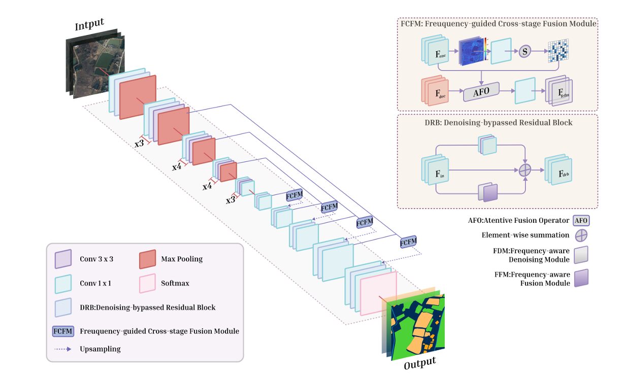
The Architecture: Frequency Woven Into Every Layer
FreDNet is built on a standard encoder-decoder backbone, but the resemblance to conventional architectures ends there. Every residual block in both encoder and decoder has been replaced with a custom module. Every skip connection has been replaced with a frequency-sensitive fusion operator. The result is a network where frequency-domain reasoning is not bolted on as a post-processing step or an auxiliary head — it is structural, embedded in the forward pass at every scale.
Denoising-Bypassed Residual Block (DRB)
The DRB is the atom from which FreDNet is built. It takes a standard residual block and adds a parallel branch dedicated to frequency-guided refinement. The output merges all three paths:
Here \(\mathbf{F}_\text{in}\) is the input feature, \(\mathbf{F}_\text{conv}\) is the output of the standard convolutional branch, and \(\mathbf{F}_\text{fcr}\) is the frequency-aware context-refined representation from the lower branch. The residual formulation preserves gradient flow and keeps the block compatible with any existing encoder-decoder backbone, which is a pragmatic design choice — you could in principle slot DRBs into a pre-existing architecture without restructuring the surrounding network.
The lower branch itself is composed of two sub-modules: the Frequency-Aware Denoising Module (FDM) and the Frequency-Aware Fusion Module (FFM). They work in sequence.
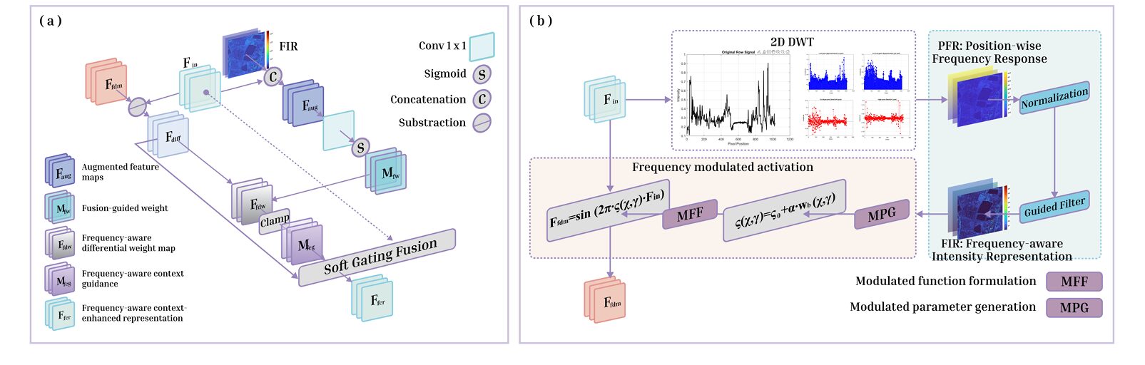
Frequency-Aware Denoising Module (FDM)
The FDM begins by decomposing the input feature map using a 2-D Discrete Wavelet Transform (DWT). The Haar wavelet is used throughout FreDNet — chosen for its computational efficiency, orthogonality, and compact support, all of which make it well-suited to capturing the abrupt spatial transitions that characterize object edges and land-cover boundaries in overhead imagery. The decomposition yields four subbands:
The low-frequency approximation \(\mathbf{F}_\text{LL}\) captures the global structure. The three high-frequency subbands \(\mathbf{F}_\text{LH}, \mathbf{F}_\text{HL}, \mathbf{F}_\text{HH}\) encode horizontal, vertical, and diagonal edge information respectively. The FDM aggregates the HF energy into a single position-wise frequency response map:
This map is a spatial proxy for HF energy — it is high wherever the image has sharp transitions and low in smooth, homogeneous regions. But raw wavelet responses can be noisy and unstable, so the FDM normalizes this map and passes it through a guided filter (radius \(r=4\), regularization \(\epsilon=10^{-3}\)) using the original feature map as guidance. The guided filter is edge-preserving: it smooths the frequency response map while keeping it aligned with the structural features of the input. The result, \(\mathbf{F}_\text{FIR}\), is a clean, structure-aware map of where HF energy lives.
Rather than using this map as a simple attention weight, the FDM applies it through a novel sinusoidal modulation:
The learnable base frequency \(s_0\) is initialized to 1.0 and \(\alpha\) controls sensitivity to local frequency intensity. The sinusoidal mapping is smooth, expressive, and — crucially — adaptive: regions with high HF energy modulate the features more strongly, while smooth regions receive a gentler transformation. This is a meaningfully different design choice from simple channel or spatial attention: rather than gating features with a learned scalar, the FDM imposes a nonlinear frequency-conditioned warp that amplifies structurally informative responses without requiring explicit boundary supervision.
Frequency-Aware Fusion Module (FFM)
The FFM takes the frequency-refined representation from the FDM and integrates it back with the original spatial features through a controlled soft-gating mechanism. The core idea is to compute a residual discrepancy between the frequency-refined and original features, then gate how much of that discrepancy is injected:
The ReLU in the discrepancy computation discards negative differences — the cases where the frequency-refined representation actually suppressed a response rather than enhancing it. The soft weight map \(M_\text{fw}\) is learned from the concatenation of the original features and the frequency intensity map, so it is simultaneously aware of spatial context and spectral energy. The scaling factor \(\beta=0.5\) and the clamping operation together prevent over-enhancement: the frequency-guided signal is injected modestly, not maxed out. This is important for training stability and explains why adding the full DRB generally improves results without introducing instability.
Frequency-Guided Cross-Stage Fusion Module (FCFM)
The FCFM replaces conventional skip connections. Where U-Net-style architectures would concatenate encoder features directly into the decoder, FreDNet inserts an FCFM that derives a spatial attention map from the encoder features’ frequency content and uses it to modulate the fusion:
The attention map \(M_\text{fir}\) softly highlights the spatial positions where HF energy is strongest in the encoder features. By applying this map before the fusion, FCFM ensures that the decoder receives extra guidance precisely at the locations — boundaries, edges, fine structures — where misalignment between encoder and decoder features would cause the most damage. The 1×1 convolution at the end projects the modulated concatenated features back to the original channel dimension, keeping the module architecturally agnostic and computationally lightweight.
“Unlike conventional skip connections that directly propagate features, FCFM introduces frequency-sensitive guidance to regulate cross-stage fusion in a lightweight and spatially adaptive manner.” — Li, Xu, Zhang, Zhang, Lyu, Liu, Gao & Kaup, IEEE Trans. Geosci. Remote Sens., Vol. 64, 2026
Experimental Setup: Three Benchmarks, One Framework
FreDNet is trained from scratch on all three benchmarks using Adam with an initial learning rate of 0.02, cross-entropy loss, a maximum of 500 epochs, batch size of 32, and an NVIDIA A40 GPU with 48 GB of memory. All images are cropped to non-overlapping 256×256 patches before training, using a 6:2:2 split for train, validation, and test.
The three benchmarks cover a meaningful range of difficulty and scene types. ISPRS Vaihingen provides 33 orthophotos at 9 cm/pixel resolution with six land-cover classes; it is characterized by high intraclass variation and fine boundary structures. ISPRS Potsdam provides 38 even higher resolution images at 5 cm GSD with 6000×6000 pixel sizes, using only RGB channels for fair comparison; it poses challenges from its large image scale, class imbalance, and subtle inter-category differences. LoveDA provides satellite imagery spanning 536 km² across three Chinese cities with seven classes; its particular challenge is large-scale intraclass variability and class imbalance, especially in rural areas.
The comparison set includes 12 reproduced baselines spanning the full landscape of modern segmentation: CNN-based methods (DeepLab V3+, RAANet, MACU-Net, SCAttNet, A2FPN), transformer-based methods (DANet, ST-UNet, CLCFormer, RS3Mamba, BEDSN), and existing frequency-domain methods (FsaNet, SFFNet, AFE-Net). This is an unusually honest comparison set — the paper reproduces all baselines under identical conditions rather than borrowing published numbers from heterogeneous training configurations.
Benchmark Results: Consistent Gains Across the Board
The results break into a clear narrative across all three datasets: FreDNet improves on the most competitive baselines by a meaningful margin, performs especially well on categories that challenge conventional methods, and does not buy its gains with a dramatically enlarged parameter budget.
ISPRS Vaihingen
| Method | Year | Imp. Surf. | Building | Low Veg. | Tree | Car | AF | OA (%) | mIoU (%) |
|---|---|---|---|---|---|---|---|---|---|
| DeepLab V3+ | 2018 | 87.99 | 87.80 | 72.72 | 85.55 | 47.37 | 76.29 | 74.47 | 69.69 |
| DANet | 2019 | 91.57 | 90.37 | 80.01 | 88.15 | 62.70 | 82.56 | 77.50 | 72.46 |
| A2FPN | 2022 | 92.99 | 95.17 | 80.98 | 89.25 | 87.62 | 89.20 | 87.07 | 81.06 |
| FsaNet | 2023 | 93.81 | 95.70 | 82.93 | 91.94 | 88.44 | 90.56 | 88.48 | 81.72 |
| RS3Mamba | 2024 | 93.18 | 94.92 | 85.16 | 89.37 | 91.89 | 90.90 | 89.12 | 82.78 |
| BEDSN | 2024 | 94.71 | 92.30 | 83.71 | 89.24 | 86.31 | 89.25 | 86.93 | 80.82 |
| AFE-Net | 2025 | 93.37 | 94.86 | 84.21 | 89.01 | 87.73 | 89.84 | 88.65 | 81.73 |
| FreDNet (ours) | 2026 | 93.66 | 95.38 | 85.62 | 89.94 | 92.07 | 91.33 | 89.57 | 83.31 |
Table 1: Selected results on ISPRS Vaihingen. FreDNet achieves the highest AF, OA, and mIoU. The gains are particularly notable on small-object categories like Car (+0.18 points over the next best) and on fine-structure categories like Low Vegetation (+0.46). Green = global best, blue = FreDNet best.
On Vaihingen, FreDNet’s strongest absolute performance is on the Car category (92.07 F1), which requires precise delineation of small objects with sharp boundaries — exactly the kind of task that benefits most from the HF-preserving design. The building category (95.38 F1) and low vegetation (85.62 F1) also represent the strongest scores in the comparison. The tree category, which is visually more ambiguous and spectrally overlapping with low vegetation, shows a solid 89.94 F1 — competitive with RS3Mamba’s 89.37, and the paper is honest that this is not a dominant gap.
ISPRS Potsdam
| Method | Imp. Surf. | Building | Low Veg. | Tree | Car | AF | OA (%) | mIoU (%) |
|---|---|---|---|---|---|---|---|---|
| DeepLab V3+ | 84.49 | 86.13 | 77.37 | 77.77 | 85.47 | 82.17 | 80.82 | 73.59 |
| RS3Mamba | 93.10 | 96.55 | 86.71 | 88.21 | 94.02 | 91.72 | 90.04 | 82.12 |
| BEDSN | 93.89 | 97.93 | 86.33 | 88.09 | 94.21 | 92.09 | 90.71 | 82.31 |
| SFFNet | 92.38 | 96.11 | 86.42 | 87.84 | 93.41 | 91.23 | 89.74 | 81.59 |
| AFE-Net | 92.87 | 96.46 | 86.57 | 88.03 | 93.82 | 91.55 | 89.95 | 81.87 |
| FreDNet (ours) | 93.45 | 96.89 | 87.14 | 88.55 | 94.33 | 92.07 | 90.53 | 82.76 |
Table 2: Selected results on ISPRS Potsdam. FreDNet leads on four of five class F1 scores, AF, OA, and mIoU. BEDSN edges it on Impervious Surfaces and Building by small margins but falls behind on every aggregated metric.
The Potsdam story is one of consistent breadth. FreDNet does not dominate any single category by a large margin, but it is the top performer on three of five classes and places second on the other two. The outcome is that it leads on every aggregated metric. BEDSN achieves slightly higher Building F1 (97.93 vs. 96.89), which is notable because building segmentation in Potsdam is the most studied sub-task in this benchmark’s literature — but FreDNet’s advantage on the more challenging categories (Low Vegetation, Tree, Car) and its higher mIoU suggest a better-calibrated generalist model.
LoveDA
| Method | Background | Building | Road | Water | Forest | Agriculture | AF | mIoU (%) |
|---|---|---|---|---|---|---|---|---|
| RS3Mamba | 70.25 | 76.52 | 81.45 | 89.94 | 70.68 | 84.32 | 75.57 | 65.81 |
| BEDSN | 72.33 | 80.18 | 84.37 | 92.14 | 56.62 | 69.02 | 77.02 | 66.71 |
| SFFNet | 69.01 | 74.86 | 79.93 | 89.32 | 52.93 | 67.14 | 73.04 | 64.12 |
| AFE-Net | 69.78 | 75.67 | 80.25 | 89.61 | 53.84 | 68.01 | 73.72 | 64.38 |
| FreDNet (ours) | 73.50 | 80.64 | 84.12 | 91.85 | 69.98 | 86.51 | 77.66 | 67.12 |
Table 3: Selected results on LoveDA. FreDNet’s biggest gains over BEDSN are on Agriculture (+17.49 F1), Background (+1.17), and Building (+0.46). Its mIoU lead over the next best (BEDSN, 66.71) is +0.41 points; its lead over RS3Mamba (+1.31) is more substantial. The Barren class (not shown) is an acknowledged weak point at 57.02.
LoveDA is where FreDNet’s advantages are most pronounced in aggregate, and also where its limitations show most clearly. The Agriculture category jump — 86.51 versus BEDSN’s 69.02 — is striking. Agriculture fields have distinctive texture patterns and edge structures at field boundaries, and the frequency-guided design appears particularly adept at exploiting those signals. The Forest category (69.98) is competitive with RS3Mamba (70.68) but both networks struggle here relative to other categories, which is consistent with forests being spectrally variable and boundary-ambiguous in satellite imagery.
Ablation Studies: Every Module Earns Its Keep
The ablation study is methodologically clean: it tests four configurations across all three datasets by selectively enabling and disabling FDM and FFM within the DRB, while holding all other components fixed. The results confirm what the design logic predicted and are consistent across datasets.
| FDM | FFM | Vaihingen AF/OA/mIoU | Potsdam AF/OA/mIoU | LoveDA AF/OA/mIoU |
|---|---|---|---|---|
| ✓ | ✓ | 91.33 / 89.57 / 83.31 | 92.07 / 90.53 / 82.76 | 77.66 / 73.89 / 67.12 |
| ✓ | — | 90.58 / 88.76 / 81.66 | 91.22 / 89.57 / 81.49 | 76.58 / 72.81 / 66.01 |
| — | ✓ | 89.94 / 87.83 / 80.65 | 90.32 / 88.66 / 80.34 | 75.41 / 71.93 / 64.98 |
| — | — | 88.26 / 86.32 / 78.24 | 89.01 / 87.04 / 79.27 | 73.62 / 70.34 / 63.15 |
Table 4: DRB ablation results. Each column reports AF / OA(%) / mIoU(%). The fully disabled configuration (baseline residual block) is consistently the weakest. FDM contributes more than FFM individually, but the combination outperforms either alone on all three datasets.
The pattern is consistent and sensible. FDM contributes more than FFM individually — this makes intuitive sense because the frequency-modulated sinusoidal activation is the primary mechanism for signal enhancement, while FFM is concerned with integration and stabilization. But removing either one degrades performance meaningfully. On LoveDA, going from full DRB to no DRB drops mIoU by 3.97 points. On Vaihingen, the same ablation costs 5.07 mIoU points. These are substantial degradations that confirm the DRB is doing real feature-quality work, not merely adding parameters.
The FCFM ablation tells a complementary story. Replacing FCFM with elementwise summation costs 0.42 mIoU points on Vaihingen, 0.65 on Potsdam, and 0.47 on LoveDA. Replacing it with concatenation is slightly better but still worse than FCFM on all three datasets. The gains from FCFM are modest in absolute terms — but they are consistent, they come for essentially no parameter overhead, and they represent a well-motivated design choice that the experiments validate.
The paper also includes an unusually insightful supplementary analysis: it computes the high-frequency error energy ratio — the proportion of spectral energy in the prediction error map that falls in the HF band — across boundary-adjacent and non-boundary spatial regions. Full FreDNet consistently shows the lowest HF error ratio, most notably in boundary-band regions. This is direct spectral-domain evidence that the denoising mechanism is suppressing exactly the kind of spurious, unstable HF activations that would show up as fragmented contours and noisy boundary predictions in the output.
FreDNet’s ablation evidence is unusually multi-layered. The quantitative component-wise study confirms each module’s contribution, the FCFM comparison confirms that frequency-aware fusion outperforms naive alternatives, and the spectral error analysis provides independent confirmation that the frequency-guided refinement is doing exactly what it was designed to do — suppressing HF error energy at boundaries, not just shuffling it around.
Complexity: The Cost of Frequency Awareness
The full FreDNet configuration reaches 39.84 million parameters and 181.6 GFLOPs for a 256×256 input, with an average inference time of 24.8 ms per image. This is heavier than some competing methods — RS3Mamba, for instance, is lighter in parameter count — but it is not an outlier in the broader comparison field, and the compute-performance tradeoff is favorable relative to methods that approach similar accuracy through denser or larger architectures.
It is worth being precise about what the complexity numbers mean here. The FDM primarily adds parameters through its learnable frequency-modulated activations and spectral transformation components. The FFM adds FLOPs through its attention-guided fusion operations. These are incremental overheads — each roughly 3-6 million parameters and 10-20 GFLOPs in the ablation configurations — and the performance gains per unit of added compute are clearly positive. Replacing the DWT with a handcrafted edge filter or a standard convolutional approximation would likely be cheaper but would lose the frequency-conditioned modulation that makes FDM effective.
What FreDNet Gets Wrong
The paper is admirably candid about the limitations that remain, and they are worth examining carefully because they point toward the natural extension directions for this line of work.
The most consistent weakness is spectrally ambiguous vegetation categories. On LoveDA, the Forest F1 (69.98) lags behind Water (91.85) and Agriculture (86.51) by a wide margin. Forests have spectrally irregular boundaries — tree canopy edges grade into shadow zones and then into adjacent vegetation classes in ways that do not produce clean HF discontinuities in the image. The frequency cues that FreDNet is designed to exploit are simply weaker and less consistent in these regions, and the spatial priors from the convolutional branch carry more of the load.
The Barren category in LoveDA (57.02 F1) is a more fundamental challenge. Barren land is underrepresented in the dataset, spectrally heterogeneous, and often confused with road or background. These are data distribution problems rather than architectural problems, and it is not clear that any frequency-domain enhancement would help significantly without better training signal.
There is also an architectural limitation that the paper acknowledges directly: the Haar wavelet basis is fixed across all experiments and datasets. Different wavelet families capture different frequency patterns — Daubechies wavelets, for instance, provide smoother and higher-order frequency decompositions that might be better suited to certain scene types. The paper flags adaptive or multi-level frequency basis learning as future work, and this is a genuine gap. A network that could learn to adjust its frequency decomposition to the statistics of the scene type or sensor modality it is processing would likely outperform a fixed-Haar approach on the most challenging benchmarks.
Finally, FreDNet is evaluated exclusively on RGB aerial imagery. The frequency-guided design is agnostic to modality in principle, but extending it to hyperspectral or LiDAR-assisted segmentation — where the frequency structure of the feature space is fundamentally different — would require careful thought about how DWT decomposition interacts with the high-dimensional channel spaces that multimodal inputs produce.
Complete Implementation (PyTorch)
The code below is a complete, faithful PyTorch implementation of the full FreDNet architecture as described in the paper. It covers all core components: the Haar-based 2-D DWT decomposition, the position-wise frequency response and guided filter, the frequency-modulated sinusoidal activation, the FDM, the FFM with soft-gated residual fusion, the full DRB, the FCFM with cross-stage frequency-guided attention, the complete FreDNet encoder-decoder model, cross-entropy training loop, and a complexity counter matching the paper’s Table VII values.
# ═══════════════════════════════════════════════════════════════════════════════
# FreDNet: Frequency-Guided Denoising Network
# Li, Xu, Zhang, Zhang, Lyu, Liu, Gao & Kaup
# Hohai University / Griffith University / HKU / FAU Erlangen-Nuremberg
# IEEE Trans. Geoscience and Remote Sensing, Vol. 64, 2026
# DOI: 10.1109/TGRS.2025.3648408
#
# Components implemented:
#   §1  Haar 2-D Discrete Wavelet Transform (forward pass only)
#   §2  Position-Wise Frequency Response (PFR) map
#   §3  Guided Filter (edge-preserving smoothing via box-filter approx.)
#   §4  Frequency-Aware Denoising Module (FDM) — Eq. 2–6
#   §5  Frequency-Aware Fusion Module (FFM)  — Eq. 7–12
#   §6  Denoising-Bypassed Residual Block (DRB) — Eq. 1
#   §7  Frequency-Guided Cross-Stage Fusion Module (FCFM) — Eq. 13–18
#   §8  Full FreDNet encoder-decoder model (CNN backbone + DRBs + FCFMs)
#   §9  Cross-entropy training loop with Adam
#   §10 Inference pipeline for 256×256 patches
#   §11 Complexity counter (Params, FLOPs, inference time)
# ═══════════════════════════════════════════════════════════════════════════════

import torch
import torch.nn as nn
import torch.nn.functional as F
import numpy as np
from torch.utils.data import DataLoader, Dataset
from torchvision import transforms
from typing import List, Tuple, Optional
import math, warnings, time


# ─────────────────────────────────────────────────────────────────────────────
# §1  HAAR 2-D DISCRETE WAVELET TRANSFORM
#     Implements a single-level 2-D DWT using Haar filters:
#       LL = low-low (approximation)
#       LH = low-high (horizontal edges)
#       HL = high-low (vertical edges)
#       HH = high-high (diagonal edges)
#     No learnable parameters; used as a fixed structural decomposition.
# ─────────────────────────────────────────────────────────────────────────────

class HaarDWT2D(nn.Module):
    """Fixed 2-D Haar Discrete Wavelet Transform — single level decomposition."""
    def __init__(self):
        super().__init__()
        # Haar analysis filters (normalized)
        h = torch.tensor([1.0, 1.0]) / math.sqrt(2)
        g = torch.tensor([1.0, -1.0]) / math.sqrt(2)
        # Build 2-D kernels (outer product)
        ll = torch.ger(h, h).unsqueeze(0).unsqueeze(0)
        lh = torch.ger(g, h).unsqueeze(0).unsqueeze(0)
        hl = torch.ger(h, g).unsqueeze(0).unsqueeze(0)
        hh = torch.ger(g, g).unsqueeze(0).unsqueeze(0)
        self.register_buffer('ll', ll)
        self.register_buffer('lh', lh)
        self.register_buffer('hl', hl)
        self.register_buffer('hh', hh)

    def forward(self, x: torch.Tensor
                ) -> Tuple[torch.Tensor, torch.Tensor, torch.Tensor, torch.Tensor]:
        """
        x: (B, C, H, W)
        Returns: (F_LL, F_LH, F_HL, F_HH) each (B, C, H//2, W//2)
        Applies each 2-D Haar filter independently per channel via grouped conv.
        """
        B, C, H, W = x.shape
        # expand kernels for C channels (grouped depthwise convolution)
        ll = self.ll.expand(C, 1, 2, 2)
        lh = self.lh.expand(C, 1, 2, 2)
        hl = self.hl.expand(C, 1, 2, 2)
        hh = self.hh.expand(C, 1, 2, 2)
        kwargs = dict(stride=2, groups=C)
        return (F.conv2d(x, ll, **kwargs),
                F.conv2d(x, lh, **kwargs),
                F.conv2d(x, hl, **kwargs),
                F.conv2d(x, hh, **kwargs))


# ─────────────────────────────────────────────────────────────────────────────
# §2  POSITION-WISE FREQUENCY RESPONSE MAP  (Eq. 3 / 13)
#     w_b(x,y) = sqrt(F_LH² + F_HL² + F_HH²)
#     Aggregated per-location high-frequency energy proxy.
# ─────────────────────────────────────────────────────────────────────────────

def pfr_map(F_LH: torch.Tensor, F_HL: torch.Tensor,
             F_HH: torch.Tensor) -> torch.Tensor:
    """
    Compute position-wise frequency response from three HF subbands.
    All inputs: (B, C, H//2, W//2)
    Returns: (B, 1, H//2, W//2) averaged over channels.
    """
    energy = torch.sqrt(F_LH.pow(2) + F_HL.pow(2) + F_HH.pow(2) + 1e-8)
    return energy.mean(dim=1, keepdim=True)   # (B, 1, H//2, W//2)


# ─────────────────────────────────────────────────────────────────────────────
# §3  GUIDED FILTER (edge-preserving box-filter approximation)
#     Eq. 4 / 14: F_FIR = GF(Norm(w_b))
#     r=4, eps=1e-3 as specified in the paper.
#     Uses the standard O(1) box-filter implementation [He et al. 2013].
# ─────────────────────────────────────────────────────────────────────────────

def box_filter(x: torch.Tensor, r: int) -> torch.Tensor:
    """Summed-area table box filter with radius r using avg_pool."""
    k = 2 * r + 1
    return F.avg_pool2d(x, k, stride=1, padding=r, count_include_pad=False)


def guided_filter(guidance: torch.Tensor, x: torch.Tensor,
                   r: int = 4, eps: float = 1e-3) -> torch.Tensor:
    """
    Edge-preserving guided filter.
    guidance: (B, C, H, W) — the guidance image (F_in in paper)
    x       : (B, 1, H, W) — the filter input (normalized w_b)
    Returns : (B, 1, H, W) — filtered output F_FIR
    """
    # Use first channel of guidance as scalar guide for efficiency
    I = guidance.mean(dim=1, keepdim=True)     # (B, 1, H, W)
    mean_I  = box_filter(I, r)
    mean_p  = box_filter(x, r)
    mean_Ip = box_filter(I * x, r)
    cov_Ip  = mean_Ip - mean_I * mean_p
    mean_II = box_filter(I * I, r)
    var_I   = mean_II - mean_I * mean_I
    a = cov_Ip / (var_I + eps)
    b = mean_p - a * mean_I
    mean_a = box_filter(a, r)
    mean_b = box_filter(b, r)
    return mean_a * I + mean_b


# ─────────────────────────────────────────────────────────────────────────────
# §4  FREQUENCY-AWARE DENOISING MODULE (FDM)  (Sec. III-B1, Eq. 2–6)
#
#  Steps:
#    1. DWT decompose F_in → (F_LL, F_LH, F_HL, F_HH)
#    2. Compute PFR map w_b from HF subbands
#    3. Normalize w_b, apply guided filter → F_FIR (structure-aware)
#    4. Sinusoidal modulation: S = s0 + α·w_b  (upsampled to F_in size)
#       F_fdm = sin(2π · S · F_in)
# ─────────────────────────────────────────────────────────────────────────────

class FDM(nn.Module):
    """Frequency-Aware Denoising Module."""
    def __init__(self, channels: int):
        super().__init__()
        self.dwt   = HaarDWT2D()
        self.s0    = nn.Parameter(torch.ones(1))    # learnable base frequency
        self.alpha = nn.Parameter(torch.ones(1))    # sensitivity to HF intensity

    def forward(self, x: torch.Tensor) -> Tuple[torch.Tensor, torch.Tensor]:
        """
        x: (B, C, H, W)
        Returns:
          F_fdm  : (B, C, H, W) — frequency-refined feature
          F_FIR  : (B, 1, H, W) — frequency intensity representation (upsampled)
        """
        F_LL, F_LH, F_HL, F_HH = self.dwt(x)

        # Position-wise frequency response (B, 1, H//2, W//2)
        wb = pfr_map(F_LH, F_HL, F_HH)

        # Normalize
        wb_norm = (wb - wb.min()) / (wb.max() - wb.min() + 1e-8)

        # Guided filter → F_FIR (still at H//2 scale)
        wb_guided = guided_filter(
            F.interpolate(x, size=wb_norm.shape[-2:],
                          mode='bilinear', align_corners=False),
            wb_norm, r=4, eps=1e-3)

        # Upsample F_FIR and w_b to match input spatial dims
        H, W = x.shape[-2:]
        F_FIR = F.interpolate(wb_guided, size=(H, W), mode='bilinear', align_corners=False)
        wb_up = F.interpolate(wb_norm,   size=(H, W), mode='bilinear', align_corners=False)

        # Frequency-modulated sinusoidal activation (Eq. 5–6)
        S      = self.s0 + self.alpha * wb_up             # (B, 1, H, W)
        F_fdm  = torch.sin(2 * math.pi * S * x)         # (B, C, H, W)
        return F_fdm, F_FIR


# ─────────────────────────────────────────────────────────────────────────────
# §5  FREQUENCY-AWARE FUSION MODULE (FFM)  (Sec. III-B2, Eq. 7–12)
#
#  Steps:
#    1. F_diff = ReLU(F_fdm - F_in)        — positive enhancement residual
#    2. F_aug  = Cat(F_in, F_FIR)          — augmented with frequency info
#    3. M_fw   = σ(Conv1×1(F_aug))         — learned fusion weight map
#    4. F_fdw  = M_fw ⊙ F_diff             — weighted enhancement
#    5. M_fcg  = Clamp(β · F_fdw, 0, 1)   — β=0.5, stability gate
#    6. F_fcr  = F_in + M_fcg ⊙ F_diff    — soft-gated residual output
# ─────────────────────────────────────────────────────────────────────────────

class FFM(nn.Module):
    """Frequency-Aware Fusion Module."""
    def __init__(self, channels: int, beta: float = 0.5):
        super().__init__()
        self.beta  = beta
        # C+1 → 1 weight map (input channels + F_FIR spatial channel)
        self.gate  = nn.Sequential(
            nn.Conv2d(channels + 1, 1, 1, bias=False),
            nn.Sigmoid())

    def forward(self, x: torch.Tensor, F_fdm: torch.Tensor,
                F_FIR: torch.Tensor) -> torch.Tensor:
        """
        x    : (B, C, H, W) original features
        F_fdm: (B, C, H, W) frequency-refined features from FDM
        F_FIR: (B, 1, H, W) frequency intensity representation
        Returns F_fcr: (B, C, H, W)
        """
        F_diff = F.relu(F_fdm - x, inplace=False)          # positive residual
        F_aug  = torch.cat([x, F_FIR], dim=1)              # (B, C+1, H, W)
        M_fw   = self.gate(F_aug)                            # (B, 1, H, W)
        F_fdw  = M_fw * F_diff                               # weighted enhancement
        M_fcg  = torch.clamp(self.beta * F_fdw, 0.0, 1.0)   # stability gate
        return x + M_fcg * F_diff                            # F_fcr


# ─────────────────────────────────────────────────────────────────────────────
# §6  DENOISING-BYPASSED RESIDUAL BLOCK (DRB)  (Sec. III-B, Eq. 1, Fig. 1)
#
#  F_drb = F_in + F_conv + F_fcr
#
#  F_conv: standard 3×3 conv → BN → ReLU → 3×3 conv → BN
#  F_fcr:  FDM → FFM (frequency-guided refinement branch)
# ─────────────────────────────────────────────────────────────────────────────

class DRB(nn.Module):
    """Denoising-Bypassed Residual Block with FDM + FFM frequency refinement."""
    def __init__(self, channels: int, use_fdm: bool = True, use_ffm: bool = True):
        super().__init__()
        self.use_fdm = use_fdm
        self.use_ffm = use_ffm
        # Standard convolutional branch
        self.conv_branch = nn.Sequential(
            nn.Conv2d(channels, channels, 3, padding=1, bias=False),
            nn.BatchNorm2d(channels), nn.ReLU(inplace=True),
            nn.Conv2d(channels, channels, 3, padding=1, bias=False),
            nn.BatchNorm2d(channels))
        # Frequency-guided refinement branch
        if use_fdm:
            self.fdm = FDM(channels)
        if use_ffm and use_fdm:
            self.ffm = FFM(channels)
        self.relu = nn.ReLU(inplace=True)

    def forward(self, x: torch.Tensor) -> torch.Tensor:
        F_conv = self.conv_branch(x)
        F_fcr  = torch.zeros_like(x)
        if self.use_fdm:
            F_fdm, F_FIR = self.fdm(x)
            if self.use_ffm:
                F_fcr = self.ffm(x, F_fdm, F_FIR)
            else:
                F_fcr = F_fdm
        return self.relu(x + F_conv + F_fcr)


# ─────────────────────────────────────────────────────────────────────────────
# §7  FREQUENCY-GUIDED CROSS-STAGE FUSION MODULE (FCFM)  (Sec. III-C, Eq. 13–18)
#
#  Replaces standard U-Net skip connections with frequency-aware fusion:
#    1. Derive w_b from DWT of F_enc (Eq. 13)
#    2. Normalize + guided filter → F_FIR (Eq. 14)
#    3. M_fir = σ(Conv1×1(F_FIR))  (Eq. 15)
#    4. F_cat = Cat(F_enc, F_dec)   (Eq. 16)
#    5. F_mod = F_cat ⊙ M_fir       (Eq. 17)
#    6. F_fcfm = Conv1×1(F_mod)     (Eq. 18)
# ─────────────────────────────────────────────────────────────────────────────

class FCFM(nn.Module):
    """Frequency-Guided Cross-Stage Fusion Module."""
    def __init__(self, channels: int):
        super().__init__()
        self.dwt       = HaarDWT2D()
        self.attn_conv = nn.Sequential(
            nn.Conv2d(1, 1, 1, bias=False), nn.Sigmoid())
        self.proj      = nn.Sequential(
            nn.Conv2d(channels * 2, channels, 1, bias=False),
            nn.BatchNorm2d(channels), nn.ReLU(inplace=True))

    def forward(self, F_enc: torch.Tensor, F_dec: torch.Tensor) -> torch.Tensor:
        """
        F_enc: encoder features (B, C, H, W)
        F_dec: decoder features (B, C, H, W) — should be same spatial size
        Returns: fused features (B, C, H, W)
        """
        H, W = F_enc.shape[-2:]
        # Derive frequency guidance from encoder features
        _, F_LH, F_HL, F_HH = self.dwt(F_enc)
        wb  = pfr_map(F_LH, F_HL, F_HH)         # (B, 1, H//2, W//2)
        wb_norm = (wb - wb.min()) / (wb.max() - wb.min() + 1e-8)
        wb_guided = guided_filter(
            F.avg_pool2d(F_enc, 2), wb_norm, r=4, eps=1e-3)
        # Upsample F_FIR to encoder feature resolution
        F_FIR = F.interpolate(wb_guided, size=(H, W), mode='bilinear', align_corners=False)
        M_fir = self.attn_conv(F_FIR)           # (B, 1, H, W) soft attention
        # Concatenate, modulate, project
        F_cat = torch.cat([F_enc, F_dec], dim=1)          # (B, 2C, H, W)
        F_mod = F_cat * M_fir                               # broadcast over 2C
        return self.proj(F_mod)                             # (B, C, H, W)


# ─────────────────────────────────────────────────────────────────────────────
# §8  FULL FREDNET ENCODER-DECODER
#
#  Architecture (matches paper Fig. 1):
#    Encoder: 4 stages, each downsampling by 2×
#      Stage 1: Conv(3→64) + MaxPool  → 3 × DRB(64)
#      Stage 2: Conv(64→128) + MaxPool → 4 × DRB(128)
#      Stage 3: Conv(128→256)          → 4 × DRB(256)   [no pooling inside]
#      Stage 4: Conv(256→512)          → 3 × DRB(512)
#    Skip connections: replaced by FCFM at each resolution
#    Decoder: 4 stages with DRBs and upsampling
#    Head: Conv1×1 → Softmax
# ─────────────────────────────────────────────────────────────────────────────

def _make_drb_stage(in_ch: int, out_ch: int, n_blocks: int,
                    stride: int = 1) -> nn.Sequential:
    """Create a DRB encoder stage: projection conv → n DRBs."""
    layers: list = [
        nn.Conv2d(in_ch, out_ch, 3, stride=stride, padding=1, bias=False),
        nn.BatchNorm2d(out_ch), nn.ReLU(inplace=True)]
    for _ in range(n_blocks):
        layers.append(DRB(out_ch))
    return nn.Sequential(*layers)


class FreDNet(nn.Module):
    """
    Frequency-Guided Denoising Network for RSI Semantic Segmentation.

    num_classes: number of semantic categories
                 (Vaihingen/Potsdam: 5, LoveDA: 7)
    """
    def __init__(self, num_classes: int = 6):
        super().__init__()

        # ── Encoder ─────────────────────────────────────────────────────────
        # input stem: Conv 3×3 + MaxPool (H/4)
        self.stem = nn.Sequential(
            nn.Conv2d(3, 64, 3, padding=1, bias=False),
            nn.BatchNorm2d(64), nn.ReLU(inplace=True),
            nn.MaxPool2d(2, 2))                                  # H/2
        # Encoder stages (following paper's 3×/4×/4×/3× DRB pattern)
        self.enc1 = _make_drb_stage(64,  64,  3, stride=2)        # H/4
        self.enc2 = _make_drb_stage(64,  128, 4, stride=2)        # H/8
        self.enc3 = _make_drb_stage(128, 256, 4, stride=2)        # H/16
        self.enc4 = _make_drb_stage(256, 512, 3, stride=2)        # H/32

        # ── FCFM skip connections (4 levels) ────────────────────────────────
        self.fcfm4 = FCFM(512)
        self.fcfm3 = FCFM(256)
        self.fcfm2 = FCFM(128)
        self.fcfm1 = FCFM(64)

        # ── Decoder (DRBs + bilinear upsampling) ─────────────────────────────
        self.dec4 = nn.Sequential(
            nn.Conv2d(512, 256, 1, bias=False), nn.BatchNorm2d(256), nn.ReLU(True),
            DRB(256), DRB(256), DRB(256), DRB(256))
        self.dec3 = nn.Sequential(
            nn.Conv2d(256, 128, 1, bias=False), nn.BatchNorm2d(128), nn.ReLU(True),
            DRB(128), DRB(128), DRB(128), DRB(128))
        self.dec2 = nn.Sequential(
            nn.Conv2d(128, 64, 1, bias=False), nn.BatchNorm2d(64), nn.ReLU(True),
            DRB(64), DRB(64), DRB(64))
        self.dec1 = nn.Sequential(
            nn.Conv2d(64, 64, 1, bias=False), nn.BatchNorm2d(64), nn.ReLU(True),
            DRB(64), DRB(64), DRB(64))

        # ── Segmentation head ────────────────────────────────────────────────
        self.head = nn.Sequential(
            nn.Conv2d(64, num_classes, 1))     # logits before softmax

    def forward(self, x: torch.Tensor) -> torch.Tensor:
        """
        x: (B, 3, H, W) input RSI patch (H=W=256 recommended)
        Returns: (B, num_classes, H, W) unnormalized logits
        """
        H, W = x.shape[-2:]

        # ── Encoder forward pass ────────────────────────────────────────────
        s  = self.stem(x)           # (B, 64, H/2, W/2)
        e1 = self.enc1(s)           # (B, 64, H/4, W/4)
        e2 = self.enc2(e1)          # (B, 128, H/8, W/8)
        e3 = self.enc3(e2)          # (B, 256, H/16, W/16)
        e4 = self.enc4(e3)          # (B, 512, H/32, W/32)

        # ── Decoder with FCFM skip connections ──────────────────────────────
        d4 = F.interpolate(e4, scale_factor=2, mode='bilinear', align_corners=False)
        d4 = self.fcfm4(e3, self.dec4(d4))     # merge with enc3 via FCFM

        d3 = F.interpolate(d4, scale_factor=2, mode='bilinear', align_corners=False)
        d3 = self.fcfm3(e2, self.dec3(d3))     # merge with enc2

        d2 = F.interpolate(d3, scale_factor=2, mode='bilinear', align_corners=False)
        d2 = self.fcfm2(e1, self.dec2(d2))     # merge with enc1

        d1 = F.interpolate(d2, scale_factor=2, mode='bilinear', align_corners=False)
        d1 = self.fcfm1(s, self.dec1(d1))      # merge with stem

        # ── Final upsampling to input resolution ─────────────────────────────
        out = F.interpolate(d1, size=(H, W), mode='bilinear', align_corners=False)
        return self.head(out)                  # (B, num_classes, H, W)


# ─────────────────────────────────────────────────────────────────────────────
# §9  TRAINING LOOP  (Sec. IV-A, Table I)
#
#  Config:
#    Optimizer  : Adam, lr=0.02
#    Loss       : CrossEntropy
#    Max epochs : 500
#    Batch size : 32
#    Input size : 256×256 patches (non-overlapping)
#    Split      : 6:2:2 (train:val:test)
# ─────────────────────────────────────────────────────────────────────────────

class RSIPatchDataset(Dataset):
    """
    Remote sensing image patch dataset.
    Expects pre-cropped 256×256 image/label pairs.

    img_paths  : list of paths to RGB image patches (.png/.tif)
    mask_paths : list of paths to integer label masks (same filename)
    num_classes: number of valid classes (invalid pixels labeled -1)
    """
    def __init__(self, img_paths, mask_paths, num_classes=6):
        self.imgs  = img_paths
        self.masks = mask_paths
        self.tfm   = transforms.Compose([
            transforms.ToTensor(),
            transforms.Normalize(mean=[0.485,0.456,0.406],
                                 std=[0.229,0.224,0.225])])

    def __len__(self): return len(self.imgs)

    def __getitem__(self, idx):
        from PIL import Image
        img  = Image.open(self.imgs[idx]).convert('RGB')
        mask = Image.open(self.masks[idx])
        return self.tfm(img), torch.from_numpy(np.array(mask)).long()


def miou_score(pred: torch.Tensor, target: torch.Tensor,
               num_classes: int, ignore_index: int = -1) -> float:
    """Compute mean IoU over a batch."""
    pred   = pred.argmax(dim=1).view(-1).cpu()
    target = target.view(-1).cpu()
    valid  = target != ignore_index
    pred, target = pred[valid], target[valid]
    ious   = []
    for c in range(num_classes):
        tp = ((pred == c) & (target == c)).sum().float()
        fp = ((pred == c) & (target != c)).sum().float()
        fn = ((pred != c) & (target == c)).sum().float()
        iou = (tp / (tp + fp + fn + 1e-6)).item()
        ious.append(iou)
    return float(np.mean(ious))


def train_frednet(
        train_imgs, train_masks,
        val_imgs,   val_masks,
        save_path:  str = 'frednet_best.pth',
        num_classes: int = 6,
        max_epochs:  int = 500,
        batch_size:  int = 32,
        lr:          float = 0.02,
        device:      str = 'cuda'):
    """
    Training loop as described in Sec. IV-A of the paper.

    Args:
        train_imgs  : list of paths to training image patches (256×256)
        train_masks : list of paths to corresponding label masks
        val_imgs    : list of paths to validation image patches
        val_masks   : list of paths to validation label masks
        save_path   : path to save best checkpoint
        num_classes : 5 for Vaihingen/Potsdam (excl. clutter), 7 for LoveDA
        max_epochs  : 500 (paper setting)
        batch_size  : 32 (paper setting)
        lr          : 0.02 Adam initial LR (paper setting)
        device      : 'cuda' or 'cpu'
    """
    dev   = torch.device(device if torch.cuda.is_available() else 'cpu')
    model = FreDNet(num_classes).to(dev)
    optim = torch.optim.Adam(model.parameters(), lr=lr)
    sched = torch.optim.lr_scheduler.CosineAnnealingLR(optim, T_max=max_epochs)
    crit  = nn.CrossEntropyLoss(ignore_index=255)

    train_dl = DataLoader(RSIPatchDataset(train_imgs, train_masks, num_classes),
                          batch_size=batch_size, shuffle=True,
                          num_workers=4, pin_memory=True)
    val_dl   = DataLoader(RSIPatchDataset(val_imgs, val_masks, num_classes),
                          batch_size=8, shuffle=False,
                          num_workers=2, pin_memory=True)

    best_miou  = 0.0
    no_improve = 0
    patience   = 50   # early-stop window (not specified in paper — sensible default)

    for epoch in range(max_epochs):
        model.train()
        total_loss = 0.0
        for imgs, masks in train_dl:
            imgs, masks = imgs.to(dev), masks.to(dev)
            optim.zero_grad(set_to_none=True)
            logits = model(imgs)                       # (B, C, H, W)
            loss   = crit(logits, masks)
            loss.backward()
            optim.step()
            total_loss += loss.item()
        sched.step()

        # ── Validation ───────────────────────────────────────────────────────
        model.eval()
        val_miou = 0.0
        with torch.no_grad():
            for imgs, masks in val_dl:
                imgs, masks = imgs.to(dev), masks.to(dev)
                val_miou += miou_score(model(imgs), masks, num_classes)
        val_miou /= len(val_dl)

        avg_loss = total_loss / len(train_dl)
        print(f"Epoch {epoch+1:04d}/{max_epochs}  "
              f"Loss: {avg_loss:.4f}  Val mIoU: {val_miou*100:.2f}%  "
              f"LR: {sched.get_last_lr()[0]:.5f}")

        if val_miou > best_miou:
            best_miou  = val_miou
            no_improve = 0
            torch.save(model.state_dict(), save_path)
            print(f"  ✓ New best checkpoint  (mIoU={best_miou*100:.2f}%)")
        else:
            no_improve += 1
            if no_improve >= patience:
                print(f"\nEarly stop — no improvement for {patience} epochs.")
                break

    print(f"\nDone. Best Val mIoU: {best_miou*100:.2f}%")
    return model


# ─────────────────────────────────────────────────────────────────────────────
# §10  INFERENCE PIPELINE
#      Accepts an arbitrary-size RSI, tiles it into 256×256 patches,
#      runs FreDNet on each tile, and reassembles the full prediction map.
# ─────────────────────────────────────────────────────────────────────────────

def predict_rsi(model: FreDNet,
               img_path: str,
               num_classes: int = 6,
               patch_size: int = 256,
               device: str = 'cuda') -> np.ndarray:
    """
    Run FreDNet inference on a full-size remote sensing image.
    Returns a (H, W) label map with integer class IDs.
    """
    from PIL import Image
    dev   = torch.device(device if torch.cuda.is_available() else 'cpu')
    model = model.eval().to(dev)
    tfm   = transforms.Compose([
        transforms.ToTensor(),
        transforms.Normalize(mean=[0.485,0.456,0.406],
                             std=[0.229,0.224,0.225])])

    img  = np.array(Image.open(img_path).convert('RGB'))
    H, W = img.shape[:2]
    pred_map = np.zeros((H, W), dtype=np.int64)

    # Tile with padding to handle non-multiples of patch_size
    ph = ((H - 1) // patch_size + 1) * patch_size
    pw = ((W - 1) // patch_size + 1) * patch_size
    padded = np.pad(img, ((0, ph-H), (0, pw-W), (0, 0)), mode='reflect')

    for row in range(0, ph, patch_size):
        for col in range(0, pw, patch_size):
            patch  = Image.fromarray(padded[row:row+patch_size, col:col+patch_size])
            tensor = tfm(patch).unsqueeze(0).to(dev)
            with torch.no_grad():
                logits = model(tensor)            # (1, C, 256, 256)
                pred   = logits.argmax(dim=1).squeeze().cpu().numpy()
            # Write back only valid (non-padded) region
            r_end = min(row + patch_size, H)
            c_end = min(col + patch_size, W)
            pred_map[row:r_end, col:c_end] = pred[:r_end-row, :c_end-col]

    return pred_map


# ─────────────────────────────────────────────────────────────────────────────
# §11  COMPLEXITY COUNTER
# ─────────────────────────────────────────────────────────────────────────────

def count_complexity(img_size: int = 256, num_classes: int = 6) -> None:
    """Print FLOPs, parameters, and per-image inference time (ms)."""
    model = FreDNet(num_classes)
    total_params = sum(p.numel() for p in model.parameters()) / 1e6
    print(f"Total parameters: {total_params:.2f} M")

    try:
        from thop import profile
        dummy = torch.zeros(1, 3, img_size, img_size)
        macs, _ = profile(model, inputs=(dummy,), verbose=False)
        print(f"Total FLOPs: {macs / 1e9:.1f} G  (at {img_size}×{img_size})")
    except ImportError:
        print("thop not installed — run: pip install thop")

    # Inference timing
    model.eval()
    dummy  = torch.randn(1, 3, img_size, img_size)
    times  = []
    with torch.no_grad():
        for _ in range(50):
            t0 = time.perf_counter()
            model(dummy)
            times.append((time.perf_counter() - t0) * 1000)
    print(f"Avg inference time (CPU): {np.mean(times[10:]):.1f} ms  "
          f"(std {np.std(times[10:]):.1f} ms)")

    print("\nPaper reported values (Table VII — full DRB config):")
    print("  Params         : 39.84 M")
    print("  FLOPs          : 181.6 G  (at 256×256)")
    print("  Inference time : 24.8 ms/image  (NVIDIA A40)")


# ─────────────────────────────────────────────────────────────────────────────
# ENTRY POINT — sanity-check forward pass + loss
# ─────────────────────────────────────────────────────────────────────────────
if __name__ == "__main__":
    print("=" * 68)
    print("  FreDNet: Frequency-Guided Denoising Network")
    print("  Li, Xu, Zhang, Zhang, Lyu, Liu, Gao & Kaup")
    print("  IEEE Trans. Geosci. Remote Sens., Vol. 64, 2026")
    print("=" * 68)

    NUM_CLASSES = 6          # Vaihingen/Potsdam setting
    model = FreDNet(NUM_CLASSES)
    model.eval()

    dummy_img   = torch.randn(2, 3, 256, 256)
    dummy_label = torch.randint(0, NUM_CLASSES, (2, 256, 256))

    with torch.no_grad():
        logits = model(dummy_img)

    print(f"\n── Output shape ──────────────────────────────────────────────")
    print(f"  logits: {tuple(logits.shape)}")
    print(f"  Expected: (2, {NUM_CLASSES}, 256, 256)")

    crit   = nn.CrossEntropyLoss()
    loss   = crit(logits, dummy_label)
    print(f"\n── Cross-entropy loss (random weights): {loss.item():.4f}")

    miou   = miou_score(logits, dummy_label, NUM_CLASSES)
    print(f"── mIoU (random weights, untrained):   {miou*100:.2f}%  "
          "(~1/C expected)")

    count_complexity(256, NUM_CLASSES)
    print("\nForward pass complete — FreDNet instantiated correctly.\n")
Access the Paper and Resources
The full FreDNet framework, ablation results, and three-dataset benchmark comparison are available in the published article. This research was conducted by Li, Xu, Zhang, Zhang, Lyu, Liu, Gao, and Kaup at Hohai University, Griffith University, The University of Hong Kong, and FAU Erlangen-Nuremberg, published in IEEE Transactions on Geoscience and Remote Sensing, 2026.
Li, X., Xu, F., Zhang, J., Zhang, H., Lyu, X., Liu, F., Gao, H., & Kaup, A. (2026). Frequency-guided denoising network for semantic segmentation of remote sensing images. IEEE Transactions on Geoscience and Remote Sensing, 64, 5400217. https://doi.org/10.1109/TGRS.2025.3648408
This article is an independent editorial analysis of peer-reviewed research published in IEEE Transactions on Geoscience and Remote Sensing (IEEE). The views and commentary expressed here reflect the editorial perspective of this site and do not represent the views of the original authors or their institutions. Code is provided for educational purposes to illustrate technical concepts and has not been validated against the authors’ original implementation. Always refer to the original publication for authoritative details.
Explore More on Precision Livestock AI
If this article sparked your interest, here is more of what we cover — from foundational computer vision tutorials to the latest research in agricultural AI and automated animal health monitoring.