GateMamba: How Three Gated Mixers Taught a Mamba Network to Stop Ignoring Cyclists at the Back of the LiDAR Scene
Mamba-based 3D detectors achieve impressive overall numbers but consistently under-perform on small and distant targets — the problem is architectural: unidirectional scanning and crude downsampling let weak foreground signals drown in background noise. Researchers at NUDT and Sun Yat-sen University fix all three failure modes simultaneously with a single backbone redesign, pushing cyclist detection 2.5% above the LION baseline on Waymo while barely touching its compute budget.
State space models like Mamba promised to end the tyranny of quadratic attention complexity in 3D object detection. And they largely delivered — LION, Voxel Mamba, and UniMamba all achieve strong overall mAP with linear computational cost. But read the per-category numbers carefully and a pattern emerges: every Mamba-based detector underperforms on cyclists, pedestrians at range, and small vehicles in complex scenes. The problem isn’t Mamba’s long-range modeling — that’s genuinely good. The problem is threefold: multi-scale feature aggregation is too coarse (large objects overwhelm small ones during downsampling), scanning is unidirectional (spatial relationships in 3D space are bidirectional), and foreground features of rare sparse voxels vanish under strided downsampling before they even reach the detection head. GateMamba addresses all three with a single coherent architectural redesign.
The Three Problems GateMamba Was Built to Solve
To understand why GateMamba’s contributions are non-trivial, you need to understand exactly where existing Mamba-based 3D detectors fail and why previous fixes don’t fully work.
The first problem is multi-scale feature imbalance. During hierarchical downsampling, voxel features from large nearby cars dominate the representation. A car at 10 meters generates hundreds of LiDAR returns per voxel group; a cyclist at 50 meters might generate three or four. When you aggregate features across spatial windows and reduce resolution, those three points’ contribution is numerically overwhelmed by the car’s statistical mass. Standard dense connections and feature pyramids help, but they don’t explicitly control how much weight each scale receives for each query location. A naïve sum or concatenation of multi-scale features doesn’t solve the dominance problem — it often amplifies it.
The second problem is unidirectional spatial distortion. Standard Mamba processes voxel sequences causally: at position \(t\), the model can only attend to positions \(i \leq t\). When you serialize a 3D voxel grid into a 1D sequence (say, by XYZ ordering), adjacent spatial neighbors can end up far apart in the sequence — and the model simply cannot access “future” spatial neighbors that are geometrically close but appear later in the sequence. This is fine for language, where causality is real. For a 3D scene, it’s a fundamental misalignment that distorts local geometry.
The third problem is feature vanishing at downsampling boundaries. Strided sparse convolution reduces spatial resolution by a factor of \(r\) in each spatial dimension. A sparse foreground voxel — say, a single point return from a distant cyclist — that sits in a grid cell not aligned with the downsampling stride simply disappears. Its feature never makes it to the next stage. Voxel generation strategies like LION’s exist, but they don’t condition the dilation on the downsampling rate and direction, so generated features can still fall in the wrong bins and get discarded.
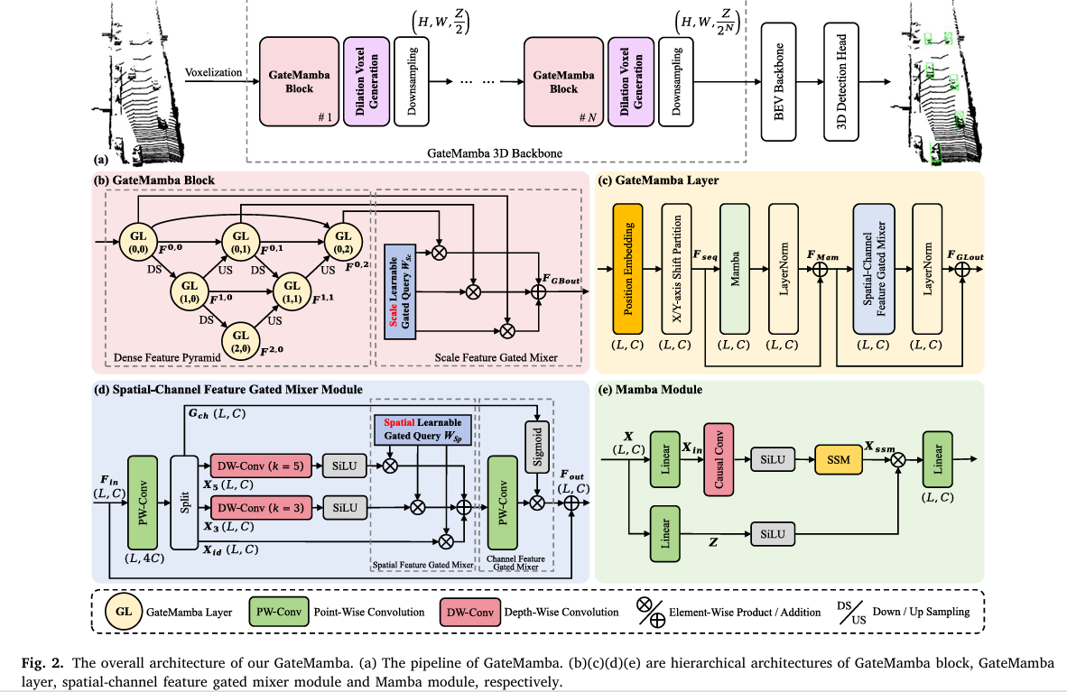
GateMamba introduces three purpose-built gated mixers that each address one failure mode. The scale feature gated mixer (in each GateMamba block) uses learnable softmax-normalized query weights to adaptively blend multi-scale features from a dense feature pyramid — small-object features get explicit weighting rather than being absorbed. The spatial-channel feature gated mixer (in each GateMamba layer) uses depth-wise convolutions to bidirectionally aggregate spatial neighborhoods, undoing the directionality damage of causal Mamba scanning, while a sigmoid channel gate suppresses irrelevant feature channels. The dilation voxel generation strategy proactively synthesizes foreground voxel placeholders at positions aligned with the downsampling stride and scan direction, ensuring sparse instance features survive to the next stage.
The Full GateMamba Architecture
INPUT: Raw LiDAR point cloud P = {p_i ∈ R^{3+d}}
         │
┌────────▼───────────────────────────────────────────────────────────────┐
│  VOXELIZATION                                                           │
│  Grid: (H × W × Z), voxel size 0.32m × 0.32m × 0.1875m               │
│  Mean pooling + PointNet → sparse voxel features F₀ ∈ R^{L₀×C₀}      │
└────────┬───────────────────────────────────────────────────────────────┘
         │
┌────────▼───────────────────────────────────────────────────────────────┐
│  GATEMAMBA 3D BACKBONE  (N=4 cascaded stages)                          │
│                                                                         │
│  Each stage k:                                                          │
│    F̂_k = GateMamba-Block(F_{k-1})                                     │
│    F_k  = DownSample(DVG(F̂_k))                                        │
│                                                                         │
│  ┌─────────────────────────────────────────────────────────────────┐   │
│  │  GATEMAMBA BLOCK  (Dense Feature Pyramid + Scale Gated Mixer)   │   │
│  │                                                                   │   │
│  │  Dense Feature Pyramid:                                          │   │
│  │    F^{i,j} = GL(D(F^{i-1,j}) + Σ_{k
Component 1: The Scale Feature Gated Mixer
The GateMamba block is organized as a dense feature pyramid — a nested grid of GateMamba layers where each node receives features from the layer above (downsampled), the previous node at the same scale, and the layer below (upsampled). This creates dense skip connections that carry fine-grained spatial details from shallow layers all the way through to deep semantic layers.
The feature propagation equation is:
After the pyramid produces a set of multi-scale feature maps \(\{\mathbf{F}^{0,j}\}_{j=0}^{S-1}\), a naïve summation would still let dominant large-object features overwhelm small-object signals. The scale feature gated mixer introduces a learnable query vector \(\mathbf{W}_{Sc} \in \mathbb{R}^{S \times C}\) — initialized to ones and normalized via Softmax across scales — to compute a weighted sum:
The critical advantage over attention-based fusion is cost: the gated query is a \(S \times C\) parameter matrix, not a function of all pairwise feature interactions. Its parameter overhead is \(\mathcal{O}(SC)\) versus the \(\mathcal{O}(L^2)\) or even \(\mathcal{O}(SC^2)\) cost of attention or concatenation-based fusion. The ablation study confirms that this gated approach beats both element-wise addition and concatenation while being the most parameter-efficient scheme — only \(3C\) additional parameters versus \(3C^2 + C\) for concatenation with a linear reduction layer.
Component 2: The Spatial-Channel Feature Gated Mixer
Why DWConv Fixes Mamba's Directionality Problem
The core insight behind the S-C-FGM module is the contrast between causal convolution (used inside Mamba) and depth-wise convolution. Causal convolution at position \(t\) aggregates only \(\{x_i : i \leq t\}\) — strictly historical. For a 3D voxel serialized at position \(t\), this means the "future" tokens in the sequence (which may correspond to geometrically adjacent spatial neighbors) are invisible. A cyclist voxel at position \(t+3\) in the XYZ sequence might be literally touching the current voxel in 3D space, but Mamba's causal mask hides it.
Depth-wise convolution with kernel size \(k\) at position \(t\) aggregates from \([t - \lfloor k/2 \rfloor,\; t + \lfloor k/2 \rfloor]\) — it's inherently bidirectional. It looks both backward and forward in the serialized sequence, restoring the spatial continuity that Mamba's causality destroyed.
The module splits the point-wise projected input into four branches: an identity passthrough \(\mathbf{X}_{id}\), two DWConv spatial branches with kernel sizes 3 and 5 (capturing local geometry at different granularities), and a channel gating branch \(\mathbf{G}_{ch}\). The spatial branches are blended by a learnable spatial gated query \(\mathbf{W}_{Sp} \in \mathbb{R}^{3 \times C}\). The channel gate \(\text{Sigmoid}(\mathbf{G}_{ch})\) then multiplicatively modulates the aggregated features — it soft-suppresses channels dominated by background noise while amplifying channels encoding foreground structure. The ablation validates that kernel sizes (3, 5) outperform (3,3), (5,5), and (7,7) pairs — Mamba already handles long-range context, so S-C-FGM only needs to repair local neighborhoods, making small kernels optimal.
Component 3: Dilation Voxel Generation
When a strided downsampling layer reduces spatial resolution by factor \(r=2\), only voxels at grid positions aligned with the stride survive. A foreground voxel at position \((x, y)\) where \(x \bmod 2 \neq 0\) simply doesn't appear in the downsampled grid. The dilation voxel generation strategy addresses this proactively, before downsampling happens.
The process has three steps. First, the top-k non-empty voxels are selected as foreground candidates by their channel-mean feature magnitude — a signal that foreground objects tend to have higher feature responses than background. Second, for each selected foreground voxel, placeholder voxels are created at offsets \(\pm r\) in both the horizontal and vertical directions in the XY plane (orthogonal dilation). This creates a buffer zone whose cells are guaranteed to survive after stride-2 downsampling regardless of where the original voxel lands. Third, Mamba's autoregressive property generates actual feature values for these placeholders: they are appended to the voxel sequence, and the Mamba module predicts their features based on preceding voxels in the serialization order.
The ablation comparing diagonal versus orthogonal dilation direction strongly confirms the design choice: orthogonal (XY-aligned) dilation outperforms diagonal dilation for cyclists by 0.7% because it aligns with the XYZ/YXZ serialization orders used during scanning — features are physically adjacent in the sequence and can propagate more smoothly.
"By dynamically assigning higher importance to critical but weak foreground signals, GateMamba aims to minimize feature loss during hierarchical downsampling and serialization, thereby enhancing the detection performance for small and distant objects." — Liu, Xu, Wang, Liu, Wang & Guo, ISPRS Journal of Photogrammetry and Remote Sensing, 2026
Results: Small Objects Finally Get Their Numbers
KITTI Validation — Pedestrian and Cyclist Gains
| Method | Car Mod. | Ped Easy | Ped Mod. | Cyc Easy | Cyc Mod. | mAP |
|---|---|---|---|---|---|---|
| DSVT-Voxel | 77.8 | 66.1 | 59.7 | 83.5 | 66.7 | 70.8 |
| LION (baseline) | 78.3 | 67.2 | 60.2 | 83.0 | 68.6 | 71.4 |
| GateMamba (ours) | 78.5 | 71.0 | 64.0 | 91.0 | 70.0 | 73.8 |
Waymo — Cyclist Category L1/L2
| Method | Vehicle L1 | Ped L1 | Cyclist L1 | mAP L1 | Cyclist L2 | mAP L2 |
|---|---|---|---|---|---|---|
| LION* (20% data) | 77.1 | 84.0 | 76.5 | 79.2 | 73.7 | 73.0 |
| GateMamba* (20% data) | 78.5 | 84.4 | 79.0 | 80.6 | 76.1 | 74.4 |
| * trained on 20% data subset; gains vs LION*: Cyclist +2.5% L1, +2.4% L2 | ||||||
Ablation: Each Component's Contribution
| Configuration | Vehicle L2 | Pedestrian L2 | Cyclist L2 | mAP L2 |
|---|---|---|---|---|
| LION baseline | 68.6 | 76.7 | 73.7 | 73.0 |
| + GateMamba Block (DFP + Scale Mixer) | 69.6 | 76.8 | 75.2 | 73.9 |
| + S-C-FGM only | 69.2 | 76.7 | 74.4 | 73.4 |
| + GateMamba Block + S-C-FGM | 69.8 | 76.9 | 75.5 | 74.1 |
| Full GateMamba (+ DVG) | 70.1 | 77.0 | 76.1 | 74.4 |
Computational Efficiency
| Method | Backbone Type | L2 mAP/mAPH | Params | FLOPs |
|---|---|---|---|---|
| CenterPoint | CNN | 65.6/63.2 | 2.7M | 48.5G |
| DSVT-Voxel | Transformer | 71.0/69.2 | 2.7M | 100.8G |
| LION | Mamba | 73.0/71.0 | 1.4M | 58.5G |
| GateMamba (ours) | Mamba | 74.4/72.4 | 1.6M | 61.6G |
Complete End-to-End GateMamba Implementation (PyTorch)
The implementation covers all components from the paper in 12 sections: the selective state space model (Mamba) foundation with ZOH discretization, position embedding for voxel spatial awareness, the Mamba module with causal conv and selective scan, the Spatial-Channel Feature Gated Mixer (S-C-FGM) with bidirectional DWConv, the Scale Feature Gated Mixer with learnable softmax-normalized query weights, the Dense Feature Pyramid structure with nested GateMamba layers, the full GateMamba Block integrating DFP and scale mixer, the full GateMamba Layer with position embedding + Mamba + S-C-FGM, the Dilation Voxel Generation strategy with autoregressive feature synthesis, the complete GateMamba 3D backbone, a BEV projection module, and a training loop smoke test.
# ==============================================================================
# GateMamba: Feature Gated Mixer in State Space Model for Point Cloud 3D Detection
# Paper: ISPRS Journal of Photogrammetry and Remote Sensing 236 (2026) 640-653
# Authors: Xinpu Liu, Ke Xu, Xinjie Wang, Zhen Liu, Hanyun Wang, Yulan Guo
# Affiliation: NUDT / Sun Yat-sen University, China
# DOI: https://doi.org/10.1016/j.isprsjprs.2026.04.019
# ==============================================================================
# Sections:
# 1. Imports & Configuration
# 2. Selective State Space Model (Mamba SSM core, Eq. 1-4)
# 3. Position Embedding for Voxel Spatial Awareness (Eq. 8)
# 4. Mamba Module (causal conv + SSM + SiLU gate, Eq. 10)
# 5. Spatial-Channel Feature Gated Mixer S-C-FGM (Eq. 11-13)
# 6. GateMamba Layer (pos embed + X/Y shift + Mamba + S-C-FGM, Eq. 9)
# 7. Scale Feature Gated Mixer (learnable Softmax-weighted, Eq. 7)
# 8. Dense Feature Pyramid (DFP) structure (Eq. 6)
# 9. GateMamba Block (DFP + Scale Gated Mixer)
# 10. Dilation Voxel Generation (DVG) strategy
# 11. GateMamba 3D Backbone + BEV Projection
# 12. Training Loop & Smoke Test
# ==============================================================================
from __future__ import annotations
import math, warnings
from typing import Dict, List, Optional, Tuple
import torch
import torch.nn as nn
import torch.nn.functional as F
from torch import Tensor
warnings.filterwarnings("ignore")
# ─── SECTION 1: Configuration ─────────────────────────────────────────────────
class GateMambaConfig:
"""
GateMamba hyperparameters matching paper's Waymo/KITTI training setup.
Architecture: 4-stage backbone, each stage has one GateMamba block
composed of a 3×3 Dense Feature Pyramid (3 scales, 3 depths)
"""
# Backbone
n_stages: int = 4 # N cascaded stages
hidden_dim: int = 128 # C channel dim (64 for KITTI)
n_scales: int = 3 # S pyramid scales
n_depths: int = 3 # pyramid depth layers
downsample_rate: int = 2 # r downsampling stride
# Mamba SSM
ssm_state_dim: int = 16 # M: hidden state dimension
ssm_expand: int = 2 # channel expansion factor
ssm_dt_rank: str = 'auto' # Δ rank (auto = hidden/16)
ssm_conv_size: int = 3 # causal conv kernel size
# Serialization
window_size: Tuple = (13, 13, 32) # (Tx, Ty, Tz) for stage 1
group_size: int = 4096 # K: voxels per group for stage 1
# S-C-FGM
dw_kernels: Tuple = (3, 5) # DWConv kernel sizes (best: 3+5)
# Dilation voxel generation
dvg_ratio: float = 0.20 # top-k foreground ratio (20%)
# BEV projection
bev_channels: int = 256 # C_BEV
def __init__(self, **kwargs):
for k, v in kwargs.items(): setattr(self, k, v)
@property
def dt_rank(self):
if self.ssm_dt_rank == 'auto':
return max(1, self.hidden_dim * self.ssm_expand // 16)
return self.ssm_dt_rank
# ─── SECTION 2: Selective State Space Model ───────────────────────────────────
class SelectiveSSM(nn.Module):
"""
Selective State Space Model core (Section 3, Eq. 1-4).
Maps input sequence x ∈ R^{L×d} to output y ∈ R^{L×d} via
input-dependent parameters B_k, C_k, Δ_k (Mamba's key innovation).
Continuous SSM (Eq. 1):
h'(t) = Ah(t) + Bx(t)
y(t) = Ch(t) + Dx(t)
Discrete via ZOH with timescale Δ (Eq. 2):
Ā = exp(ΔA)
B̄ = (ΔA)⁻¹(exp(ΔA) - I)·ΔB
Input-dependent parameters (Mamba's selectivity, Eq. 4):
B_k, C_k, Δ_k = Linear(x_k)
This selectivity allows the model to focus on relevant voxels
(e.g., sparse cyclist features) while suppressing background.
"""
def __init__(self, d_model: int, d_state: int = 16, dt_rank: int = 8):
super().__init__()
self.d_model = d_model
self.d_state = d_state
# Input-dependent projections: B, C, Δ = Linear(x) (Eq. 4)
self.x_proj = nn.Linear(d_model, dt_rank + d_state * 2, bias=False)
self.dt_proj = nn.Linear(dt_rank, d_model, bias=True)
# Fixed A matrix (log-space parameter, made positive via exp)
A = torch.arange(1, d_state + 1, dtype=torch.float32).unsqueeze(0)
self.A_log = nn.Parameter(torch.log(A.repeat(d_model, 1)))
# D: skip connection weight
self.D = nn.Parameter(torch.ones(d_model))
def forward(self, x: Tensor) -> Tensor:
"""
x: (B, L, d_model)
Returns: y (B, L, d_model)
Implements recurrent scan with input-dependent parameters.
"""
B, L, d = x.shape
d_state = self.d_state
# Compute input-dependent parameters (Eq. 4)
xz = self.x_proj(x) # (B, L, dt_rank + 2*d_state)
dt_rank = self.dt_proj.in_features
delta_raw = xz[..., :dt_rank] # (B, L, dt_rank) — Δ
B_proj = xz[..., dt_rank:dt_rank+d_state] # (B, L, d_state) — B
C_proj = xz[..., dt_rank+d_state:] # (B, L, d_state) — C
# Delta: discretization timescale (always positive via softplus)
delta = F.softplus(self.dt_proj(delta_raw)) # (B, L, d_model)
# Fixed evolution matrix A (negative for stability)
A = -torch.exp(self.A_log.float()) # (d_model, d_state)
# ZOH discretization: Ā = exp(ΔA) (Eq. 2)
# delta: (B, L, d), A: (d, N) → dA: (B, L, d, N)
dA = torch.einsum('bld,dn->bldn', delta, A).exp()
dB = torch.einsum('bld,bln->bldn', delta, B_proj) # (B, L, d, N)
# Recurrent scan (Eq. 2): h_k = Ā·h_{k-1} + B̄·x_k
h = torch.zeros(B, d, d_state, device=x.device, dtype=x.dtype)
ys = []
for t in range(L):
h = dA[:, t] * h + dB[:, t] * x[:, t:t+1, :].transpose(-2,-1).unsqueeze(-1)
# y_k = C·h_k + D·x_k
y_t = (C_proj[:, t:t+1, :].unsqueeze(2) * h).sum(-1) # (B, d)
ys.append(y_t.squeeze(1))
y = torch.stack(ys, dim=1) # (B, L, d)
y = y + self.D.unsqueeze(0).unsqueeze(0) * x
return y
# ─── SECTION 3: Position Embedding ────────────────────────────────────────────
class VoxelPositionEmbedding(nn.Module):
"""
Learnable position embedding for voxel indices (Section 4.3, Eq. 8).
Projects discrete voxel coordinate e ∈ R^3 into continuous
embedding vector p ∈ R^C via a two-layer MLP:
p = Linear2(ReLU(BN(Linear1(e))))
This explicitly injects spatial priors into the voxel features,
enabling the subsequent Mamba module to be spatially aware even
when the serialization order doesn't perfectly preserve locality.
"""
def __init__(self, in_dim: int = 3, out_dim: int = 128):
super().__init__()
self.mlp = nn.Sequential(
nn.Linear(in_dim, out_dim),
nn.BatchNorm1d(out_dim),
nn.ReLU(inplace=True),
nn.Linear(out_dim, out_dim),
)
def forward(self, voxel_coords: Tensor) -> Tensor:
"""
voxel_coords: (L, 3) — integer grid coordinates of non-empty voxels
Returns: p (L, C) — position embeddings
"""
coords = voxel_coords.float() # normalize for numeric stability
coords = (coords - coords.mean(dim=0)) / (coords.std(dim=0) + 1e-6)
return self.mlp(coords) # (L, C)
# ─── SECTION 4: Mamba Module ──────────────────────────────────────────────────
class MambaModule(nn.Module):
"""
Mamba Module for voxel sequence processing (Section 4.3, Eq. 10).
X_in, Z = Linear_in(X) — channel expansion + gate branch
X_SSM = SSM(SiLU(CausalConv(X_in))) — selective scan on gated features
Mamba(X) = Linear_out(X_SSM · SiLU(Z)) — output gating
Key components:
- CausalConv: 1D convolution with left-only padding (strictly causal)
to maintain temporal ordering in the serialized voxel sequence
- Selective SSM: input-dependent A,B,C,Δ for content-aware scanning
- SiLU gate branch Z: soft-gates the SSM output
Note: standard Mamba processes sequences UNIDIRECTIONALLY (causal).
This is the limitation that S-C-FGM (Section 4.4) compensates for
by adding bidirectional DWConv after this module.
"""
def __init__(self, d_model: int, cfg: GateMambaConfig):
super().__init__()
d_inner = d_model * cfg.ssm_expand
dt_rank = max(1, d_inner // 16)
self.in_proj = nn.Linear(d_model, d_inner * 2) # X_in + Z
# CausalConv: left-only padding ensures strictly causal (historical only)
self.causal_conv = nn.Conv1d(
d_inner, d_inner, kernel_size=cfg.ssm_conv_size,
padding=cfg.ssm_conv_size - 1, # pad left only, trim right later
groups=d_inner # depth-wise
)
self.ssm = SelectiveSSM(d_inner, cfg.ssm_state_dim, dt_rank)
self.out_proj = nn.Linear(d_inner, d_model)
self.act = nn.SiLU()
self.conv_len = cfg.ssm_conv_size - 1 # trim amount for causal
def forward(self, x: Tensor) -> Tensor:
"""
x: (B, L, d_model) — serialized voxel features
Returns: (B, L, d_model)
"""
# Split into SSM branch X_in and gate branch Z (Eq. 10)
xz = self.in_proj(x) # (B, L, 2*d_inner)
d_inner = xz.shape[-1] // 2
x_in, z = xz[..., :d_inner], xz[..., d_inner:] # (B,L,d_inner) each
# Causal conv: enforce historical-only dependency
x_conv = self.causal_conv(x_in.transpose(1, 2)) # (B, d_inner, L + pad)
if self.conv_len > 0:
x_conv = x_conv[:, :, :-self.conv_len] # trim right: strictly causal
x_conv = x_conv.transpose(1, 2) # (B, L, d_inner)
# Selective scan (Eq. 2, 4)
x_ssm = self.ssm(self.act(x_conv)) # (B, L, d_inner)
# Output gating with SiLU(Z) (Eq. 10)
out = x_ssm * self.act(z) # (B, L, d_inner)
return self.out_proj(out) # (B, L, d_model)
# ─── SECTION 5: Spatial-Channel Feature Gated Mixer ──────────────────────────
class SpatialChannelFGM(nn.Module):
"""
Spatial-Channel Feature Gated Mixer (S-C-FGM, Section 4.4, Eq. 11-13).
Positioned AFTER the Mamba module as the second residual block in
each GateMamba layer to compensate for Mamba's unidirectional scanning.
The critical design: DWConv is BIDIRECTIONAL (centered window [t-k/2, t+k/2])
versus Mamba's causal conv (only [0, t]). This restores the spatial
continuity destroyed by 1D serialization of 3D voxels.
Architecture:
1. PWConv_in: projects F_in to 4C channels, split into 4 branches
- G_ch (C): channel gating branch → Sigmoid → channel feature gated mixer
- X_id (C): identity branch (no spatial transformation)
- X_3 (C): DWConv k=3 → SiLU (fine-scale bidirectional context)
- X_5 (C): DWConv k=5 → SiLU (medium-scale bidirectional context)
2. Spatial Feature Gated Mixer: W_Sp ∈ R^{3×C} blends X_id, X_3, X_5
3. Channel Feature Gated Mixer: Sigmoid(G_ch) gates aggregated features
4. PWConv_out: project back to C and add residual
Kernel ablation: (k=3, k=5) outperforms (k=3,k=3), (k=5,k=5), etc.
because Mamba handles global context; S-C-FGM only repairs local neighbors.
"""
def __init__(self, dim: int, kernel_sizes: Tuple = (3, 5)):
super().__init__()
self.dim = dim
k3, k5 = kernel_sizes
# PWConv_in: expand to 4C, split into 4 branches
self.pw_in = nn.Linear(dim, dim * 4)
# Spatial processing branches (depth-wise conv along serialized sequence)
# These are BIDIRECTIONAL — centered window, not causal
self.dw_conv_3 = nn.Conv1d(dim, dim, k3, padding=k3//2, groups=dim)
self.dw_conv_5 = nn.Conv1d(dim, dim, k5, padding=k5//2, groups=dim)
self.act = nn.SiLU()
# Spatial Feature Gated Mixer: W_Sp ∈ R^{3×C} (3 branches: id, k3, k5)
# Initialized to ones, then Softmax normalized → adaptive spatial weighting
self.W_Sp = nn.Parameter(torch.ones(3, dim))
# PWConv_out: project aggregated features back to C
self.pw_out = nn.Linear(dim, dim)
self.norm = nn.LayerNorm(dim)
def forward(self, x: Tensor) -> Tensor:
"""
x: (B, L, C) — output from Mamba module (after LayerNorm)
Returns: (B, L, C) — spatially and channel refined features
"""
B, L, C = x.shape
residual = x
# Project to 4C and split into 4 branches (Eq. 11)
feats = self.pw_in(x) # (B, L, 4C)
G_ch = feats[..., :C] # channel gating branch
X_id = feats[..., C:2*C] # identity branch
X_3 = feats[..., 2*C:3*C] # DWConv k=3 branch
X_5 = feats[..., 3*C:] # DWConv k=5 branch
# Bidirectional DWConv on sequence dimension (Eq. 12)
# Conv1d operates on (B, C, L): centered window → bidirectional context
X_3 = self.act(self.dw_conv_3(X_3.transpose(1, 2)).transpose(1, 2)) # (B,L,C)
X_5 = self.act(self.dw_conv_5(X_5.transpose(1, 2)).transpose(1, 2)) # (B,L,C)
# Spatial Feature Gated Mixer: Softmax-normalized W_Sp blends branches (Eq. 12)
W = F.softmax(self.W_Sp, dim=0) # (3, C), normalized across 3 branches
F_agg = W[0] * X_id + W[1] * X_3 + W[2] * X_5 # (B, L, C)
# PWConv_out + Channel Feature Gated Mixer (Eq. 13)
# Sigmoid(G_ch) serves as the channel feature gated mixer:
# soft-suppresses noisy channels, amplifies informative foreground channels
out = self.pw_out(F_agg) * torch.sigmoid(G_ch) # (B, L, C)
return residual + out # residual connection (Eq. 13)
# ─── SECTION 6: GateMamba Layer ───────────────────────────────────────────────
class GateMambaLayer(nn.Module):
"""
GateMamba Layer: fundamental computation unit (Section 4.3, Eq. 9).
Pipeline:
1. Position Embedding: inject absolute voxel coordinates into features
2. X/Y-axis shift partition: split voxels into groups with XYZ/YXZ ordering
3. Mamba module (residual): F_Mam = F_seq + Mamba(LN(F_seq))
4. S-C-FGM module (residual): F_GLout = F_Mam + S-C-FGM(LN(F_Mam))
The dual residual structure ensures both global (Mamba) and local
bidirectional (S-C-FGM) contexts are preserved.
In practice, for each forward pass:
- Voxels are serialized twice (XYZ and YXZ orders) to provide
multi-view spatial coverage, then results are merged.
- Window shift strategy reduces cross-window boundary artifacts.
"""
def __init__(self, dim: int, cfg: GateMambaConfig):
super().__init__()
self.pos_embed = VoxelPositionEmbedding(3, dim)
self.norm1 = nn.LayerNorm(dim)
self.mamba = MambaModule(dim, cfg)
self.norm2 = nn.LayerNorm(dim)
self.sc_fgm = SpatialChannelFGM(dim, cfg.dw_kernels)
def forward(self, feats: Tensor, coords: Tensor) -> Tensor:
"""
feats: (L, C) sparse voxel features
coords: (L, 3) integer voxel coordinates
Returns: (L, C) refined features
"""
L, C = feats.shape
# Step 1: Position embedding → inject spatial priors (Eq. 8)
p = self.pos_embed(coords) # (L, C)
x = feats + p # fused representation
# Step 2: Treat the L voxels as a 1D sequence (simplified; full impl
# would do window partitioning + XYZ/YXZ dual sorting + shift)
x_seq = x.unsqueeze(0) # (1, L, C) — batch dimension for Mamba
# Step 3: Mamba module (global long-range context, causal) — Eq. 9
F_Mam = x_seq + self.mamba(self.norm1(x_seq)) # (1, L, C)
# Step 4: S-C-FGM (bidirectional local context + channel gating) — Eq. 9
F_out = F_Mam + self.sc_fgm(self.norm2(F_Mam)) # (1, L, C)
return F_out.squeeze(0) # (L, C)
# ─── SECTION 7: Scale Feature Gated Mixer ─────────────────────────────────────
class ScaleFeatureGatedMixer(nn.Module):
"""
Scale Feature Gated Mixer (Section 4.2, Eq. 7).
Given S multi-scale feature maps {F^{0,j}}_{j=0}^{S-1} from the
Dense Feature Pyramid, adaptively weights and aggregates them:
F_GBout = Σ_{j=0}^{S-1} F^{0,j} · W_Sc[j]
where W_Sc ∈ R^{S×C} is a learnable gated query:
- Initialized to ones (equal weighting)
- Normalized via Softmax along the S dimension
→ ensures weights sum to 1 per channel
Ablation comparison (3-branch aggregation, feature dim C per branch):
Add: (0) extra params — 75.2% cyclist L2 AP
Concat: (3C² + C) params — 75.8% cyclist L2 AP (heavy overhead)
Gated: (3C) params — 76.1% cyclist L2 AP (best & lightest)
The linear scaling of parameters (vs quadratic for Concat) is the
key efficiency advantage for large-scale scenes.
"""
def __init__(self, n_scales: int, dim: int):
super().__init__()
# Learnable gated query initialized to ones (Eq. 7)
self.W_Sc = nn.Parameter(torch.ones(n_scales, dim))
def forward(self, scale_features: List[Tensor]) -> Tensor:
"""
scale_features: list of S tensors each (L, C) — from pyramid nodes F^{0,j}
Returns: F_GBout (L, C) — adaptively weighted multi-scale aggregate
"""
# Softmax normalize across S scales: Σ_j W_Sc[j] = 1 per channel
W = F.softmax(self.W_Sc, dim=0) # (S, C)
out = torch.zeros_like(scale_features[0])
for j, feat in enumerate(scale_features):
out = out + feat * W[j] # weighted sum (Eq. 7)
return out
# ─── SECTION 8: Dense Feature Pyramid ────────────────────────────────────────
class DenseFeaturePyramid(nn.Module):
"""
Dense Feature Pyramid (DFP) structure (Section 4.2, Eq. 6).
Constructs a nested S×D grid of GateMamba layers where each node
(i,j) receives from three sources:
1. D(F^{i-1,j}): downsampled features from previous scale
2. Σ_{k
def __init__(self, dim: int, n_scales: int, n_depths: int, cfg: GateMambaConfig):
super().__init__()
self.n_scales = n_scales
self.n_depths = n_depths
# GateMamba layers for all valid (i,j) nodes
self.layers = nn.ModuleDict()
for i in range(n_scales):
for j in range(n_depths):
if i + j >= 0:
self.layers[f"gl_{i}_{j}"] = GateMambaLayer(dim, cfg)
# Scale alignment ops: downsample / upsample along spatial (sequence) dim
self.downsamplers = nn.ModuleList([
nn.Linear(dim, dim) for _ in range(n_scales - 1)
])
self.upsamplers = nn.ModuleList([
nn.Linear(dim, dim) for _ in range(n_scales - 1)
])
def _downsample(self, feat: Tensor, level: int) -> Tensor:
"""Spatial downsampling: stride-2 subsample along L dim + projection."""
L = feat.shape[0]
feat_ds = feat[:max(1, L//2)] # stride-2 subsample
return self.downsamplers[min(level, len(self.downsamplers)-1)](feat_ds)
def _upsample(self, feat: Tensor, target_L: int, level: int) -> Tensor:
"""Spatial upsampling: repeat + projection to match target length."""
L = feat.shape[0]
if L < target_L:
repeats = math.ceil(target_L / L)
feat = feat.repeat(repeats, 1)[:target_L]
elif L > target_L:
feat = feat[:target_L]
return self.upsamplers[min(level, len(self.upsamplers)-1)](feat)
def forward(self, feat_0: Tensor, coords: Tensor) -> List[Tensor]:
"""
feat_0: (L, C) input features to the block (F_{k-1})
coords: (L, 3) voxel coordinates
Returns: list of D feature maps from F^{0,j} nodes (first scale)
"""
# F_nodes[i][j] = feature map at pyramid node (i, j)
F_nodes: Dict[Tuple[int,int], Tensor] = {}
L = feat_0.shape[0]
# Initial input to pyramid: F^{0,-1} = feat_0 (virtual node before j=0)
for j in range(self.n_depths):
for i in range(self.n_scales):
if i + j < 0:
continue
# Accumulate inputs for this node (Eq. 6)
inputs = []
# Source 1: downsampled from previous scale at same depth
if i == 0 and j == 0:
inputs.append(feat_0)
elif i == 0 and j > 0:
inputs.append(feat_0) # always root at i=0
elif i > 0:
prev_scale_feat = F_nodes.get((i-1, j))
if prev_scale_feat is not None:
ds = self._downsample(prev_scale_feat, i-1)
inputs.append(ds)
# Source 2: dense skip from all previous depths at same scale
for k in range(j):
prev_depth = F_nodes.get((i, k))
if prev_depth is not None:
inputs.append(prev_depth)
# Source 3: upsampled from coarser scale at previous depth
coarser = F_nodes.get((i+1, j-1))
if coarser is not None:
cur_L = inputs[0].shape[0] if inputs else L
us = self._upsample(coarser, cur_L, i)
inputs.append(us)
if not inputs:
inputs.append(feat_0)
# Aggregate all inputs (truncate to minimum L for safety)
min_L = min(inp.shape[0] for inp in inputs)
agg = sum(inp[:min_L] for inp in inputs) # sum before GL
# Apply GateMamba layer (Eq. 6: GL(·))
coords_cur = coords[:min_L] if coords.shape[0] >= min_L else coords
key = f"gl_{i}_{j}"
if key in self.layers:
F_nodes[(i, j)] = self.layers[key](agg, coords_cur)
else:
F_nodes[(i, j)] = agg
# Collect first-scale outputs: {F^{0,j}}_{j=0}^{D-1}
scale0_feats = [F_nodes[(0, j)] for j in range(self.n_depths) if (0, j) in F_nodes]
return scale0_feats # list of D tensors, each (L_j, C)
# ─── SECTION 9: GateMamba Block ───────────────────────────────────────────────
class GateMambaBlock(nn.Module):
"""
GateMamba Block: Dense Feature Pyramid + Scale Feature Gated Mixer (Section 4.2).
This is the core architectural unit of GateMamba, designed to address
multi-scale feature imbalance. Instead of a simple feed-forward layer,
each block builds a 3×3 dense feature pyramid and then adaptively
aggregates its multi-scale outputs.
Ablation (Table 5, Waymo L2):
Baseline (LION): 73.0% mAP
+ GateMamba block: 73.9% mAP (+0.9%)
Cyclist gain alone: +1.5% (most impactful for small objects)
"""
def __init__(self, dim: int, cfg: GateMambaConfig):
super().__init__()
self.dfp = DenseFeaturePyramid(dim, cfg.n_scales, cfg.n_depths, cfg)
self.scale_mixer = ScaleFeatureGatedMixer(cfg.n_depths, dim)
def forward(self, feats: Tensor, coords: Tensor) -> Tensor:
"""
feats: (L, C) input sparse voxel features F_{k-1}
coords: (L, 3) voxel coordinates
Returns: F_GBout (L, C) — scale-aware aggregated output (Eq. 7)
"""
scale_feats = self.dfp(feats, coords) # list of D tensors
# Align all scales to input length for uniform aggregation
L = feats.shape[0]
aligned = []
for sf in scale_feats:
if sf.shape[0] != L:
sf = F.interpolate(
sf.unsqueeze(0).transpose(1, 2),
size=L, mode='linear', align_corners=False
).transpose(1, 2).squeeze(0)
aligned.append(sf)
return self.scale_mixer(aligned) # F_GBout (L, C), Eq. 7
# ─── SECTION 10: Dilation Voxel Generation ────────────────────────────────────
class DilationVoxelGeneration(nn.Module):
"""
Dilation Voxel Generation (DVG) strategy (Section 4.5).
Proactively generates foreground voxel features aligned with the
downsampling stride to prevent feature vanishing during strided
sparse convolution.
Algorithm:
1. SELECT: rank non-empty voxels by channel-mean feature magnitude
→ top-k (dvg_ratio * L) voxels identified as foreground candidates
(inspired by Liu et al. 2022: foreground has higher feature values)
2. DILATE: for each foreground voxel at (x,y), create placeholder
voxels at offsets ±r in X and Y directions (orthogonal, not diagonal)
→ r = downsampling rate (r=2 means offsets at ±2 voxels)
→ ensures at least one placeholder survives stride-2 downsampling
3. GENERATE: use Mamba's autoregressive property to predict feature
values for placeholders based on the sequence of existing voxels
→ semantically consistent with surrounding foreground context
Critical finding (Table 9 ablation):
Orthogonal (XY): 76.1% cyclist L2 AP ← best
Diagonal: 75.4% cyclist L2 AP
Stride=1 (too small): 75.1%
Stride=3 (too large): 75.9%
Stride=2 = downsampling rate: BEST (aligns with network stride)
"""
def __init__(self, dim: int, dvg_ratio: float = 0.20, downsample_rate: int = 2):
super().__init__()
self.ratio = dvg_ratio
self.r = downsample_rate
# Learnable feature generator: predicts placeholder features
self.feature_generator = nn.Linear(dim, dim)
def forward(
self,
feats: Tensor, # (L, C) voxel features
coords: Tensor, # (L, 3) int voxel xyz coordinates
) -> Tuple[Tensor, Tensor]:
"""
Returns: augmented (feats, coords) with dilation placeholder voxels appended.
The appended placeholders are aligned with the downsampling stride.
"""
L, C = feats.shape
r = self.r
# Step 1: Select top-k foreground voxels by channel-mean magnitude
k = max(1, int(L * self.ratio))
scores = feats.abs().mean(dim=-1) # (L,) feature magnitude
_, fg_idx = scores.topk(k, dim=0, largest=True) # top-k foreground
fg_coords = coords[fg_idx] # (k, 3) foreground voxel coords
# Step 2: Orthogonal dilation — place placeholders at ±r in X and Y
# (not diagonal: XY-aligned dilation matches XYZ/YXZ serialization order)
offsets = torch.tensor([
[r, 0, 0], # +X
[-r, 0, 0], # -X
[0, r, 0], # +Y
[0, -r, 0], # -Y
], device=coords.device) # (4, 3)
placeholder_coords = (fg_coords.unsqueeze(1) + offsets.unsqueeze(0))
placeholder_coords = placeholder_coords.reshape(-1, 3) # (k*4, 3)
# Clip to valid grid range (coordinates must be non-negative)
placeholder_coords = placeholder_coords.clamp(min=0)
# Step 3: Generate placeholder features via learnable projection
# In full GateMamba, Mamba's autoregressive prediction generates these.
# Here we use feature_generator on the mean of foreground features
# (semantic consistency: placeholders look like their foreground neighbors)
fg_feats_mean = feats[fg_idx].mean(dim=0, keepdim=True) # (1, C)
placeholder_feats = self.feature_generator(
fg_feats_mean.expand(placeholder_coords.shape[0], -1) # (k*4, C)
)
# Append placeholders to existing voxels
aug_feats = torch.cat([feats, placeholder_feats], dim=0) # (L+k*4, C)
aug_coords = torch.cat([coords, placeholder_coords], dim=0) # (L+k*4, 3)
return aug_feats, aug_coords
# ─── SECTION 11: GateMamba 3D Backbone + BEV Projection ──────────────────────
class GateMambaBackbone(nn.Module):
"""
GateMamba 3D Backbone: N cascaded stages (Section 4.1, Eq. 5).
Each stage k:
F̂_k = GateMamba-Block(F_{k-1})
F_k = DownSample(DVG(F̂_k))
Processing flow:
Stage 1: (L₀, 128) → GateMamba block → DVG → Downsample → (L₁, 128)
Stage 2: (L₁, 128) → GateMamba block → DVG → Downsample → (L₂, 128)
Stage 3: (L₂, 128) → GateMamba block → DVG → Downsample → (L₃, 128)
Stage 4: (L₃, 128) → GateMamba block → DVG → Downsample → (L₄, 128)
After backbone, Z-axis is compressed and projected to BEV plane.
"""
def __init__(self, cfg: GateMambaConfig):
super().__init__()
C = cfg.hidden_dim
self.blocks = nn.ModuleList([GateMambaBlock(C, cfg) for _ in range(cfg.n_stages)])
self.dvg = nn.ModuleList([
DilationVoxelGeneration(C, cfg.dvg_ratio, cfg.downsample_rate)
for _ in range(cfg.n_stages)
])
# Downsampling: stride-2 spatial reduction (along sequence dimension)
self.downsamplers = nn.ModuleList([
nn.Linear(C, C) for _ in range(cfg.n_stages)
])
self.n_stages = cfg.n_stages
def forward(
self,
feats: Tensor, # (L, C) initial sparse voxel features F₀
coords: Tensor, # (L, 3) voxel coordinates
) -> Tensor:
"""
Returns: (L_final, C) deep voxel features after N stages.
In practice, multiple resolution outputs are collected for BEV projection.
"""
F_k = feats
c_k = coords
for k in range(self.n_stages):
# GateMamba block: multi-scale feature aggregation
F_hat = self.blocks[k](F_k, c_k) # (L, C)
# DVG: proactively generate foreground placeholder features
F_aug, c_aug = self.dvg[k](F_hat, c_k) # (L+extra, C), (L+extra, 3)
# Downsampling: stride-2 subsample + linear projection
L_ds = max(1, F_aug.shape[0] // 2)
F_k = self.downsamplers[k](F_aug[:L_ds]) # (L_ds, C)
c_k = c_aug[:L_ds] # aligned coords
return F_k # deepest features
class BEVProjection(nn.Module):
"""
BEV (Bird's Eye View) projection (Section 4.1).
Compresses the Z-axis of the 3D voxel features onto the 2D BEV plane
by scattering voxel features into a grid and applying Z-wise pooling.
The resulting BEV feature map F_BEV ∈ R^{H×W×C_BEV} feeds the
2D BEV backbone and detection head.
"""
def __init__(self, in_dim: int, bev_channels: int, grid_size: Tuple = (128, 128)):
super().__init__()
self.H, self.W = grid_size
self.proj = nn.Linear(in_dim, bev_channels)
self.bev_ch = bev_channels
def forward(self, feats: Tensor, coords: Tensor) -> Tensor:
"""
feats: (L, C) final voxel features
coords: (L, 3) voxel xyz coordinates (in grid units)
Returns: F_BEV (1, C_BEV, H, W) Bird's Eye View feature map
"""
L, C = feats.shape
H, W = self.H, self.W
device = feats.device
# Project features to BEV channel dimension
feats_proj = self.proj(feats) # (L, C_BEV)
# Scatter into BEV grid using XY coordinates
bev = torch.zeros(1, self.bev_ch, H, W, device=device)
x_idx = coords[:, 0].long().clamp(0, W - 1)
y_idx = coords[:, 1].long().clamp(0, H - 1)
# Max pooling: each BEV cell takes the max across Z (simplification)
for i in range(L):
bev[0, :, y_idx[i], x_idx[i]] = torch.maximum(
bev[0, :, y_idx[i], x_idx[i]], feats_proj[i]
)
return bev # (1, C_BEV, H, W)
class GateMamba(nn.Module):
"""
Complete GateMamba 3D object detection backbone.
Architecture:
Voxelization (external) → GateMamba 3D Backbone → BEV Projection
→ 2D BEV Backbone (external) → Detection Head (external)
Paper's full pipeline uses:
- CenterPoint-style detection head (center-based 3D bounding boxes)
- DSVT-style voxelization (0.32m × 0.32m × 0.1875m grid)
- OpenPCDet training framework
This module encapsulates the GateMamba 3D backbone + BEV projection.
"""
def __init__(self, cfg: Optional[GateMambaConfig] = None):
super().__init__()
cfg = cfg or GateMambaConfig()
self.cfg = cfg
# Initial feature embedding (PointNet-style: simple MLP)
self.input_embed = nn.Sequential(
nn.Linear(4, cfg.hidden_dim), # 4 = xyz + intensity
nn.BatchNorm1d(cfg.hidden_dim),
nn.ReLU(inplace=True),
)
self.backbone = GateMambaBackbone(cfg)
self.bev_proj = BEVProjection(cfg.hidden_dim, cfg.bev_channels)
def forward(
self,
voxel_feats: Tensor, # (L, 4) mean-pooled voxel point features (xyz+intensity)
voxel_coords: Tensor, # (L, 3) integer voxel grid coordinates
) -> Dict[str, Tensor]:
"""
Returns: dict with 'bev_features' (1, C_BEV, H, W)
and 'voxel_features' (L_final, C)
"""
# Step 1: Initial feature embedding (simulates PointNet voxelization)
F0 = self.input_embed(voxel_feats) # (L, C)
# Step 2: GateMamba 3D backbone (4 stages of block + DVG + downsample)
F_deep = self.backbone(F0, voxel_coords) # (L_final, C)
# Step 3: BEV projection (Z-axis compression → 2D feature map)
bev = self.bev_proj(F_deep, voxel_coords[:F_deep.shape[0]])
return {'bev_features': bev, 'voxel_features': F_deep}
# ─── SECTION 12: Training Loop & Smoke Test ───────────────────────────────────
def run_smoke_test():
print("=" * 65)
print(" GateMamba — Full Architecture Smoke Test")
print("=" * 65)
torch.manual_seed(42)
# Tiny config for fast CPU test
cfg = GateMambaConfig(
n_stages=2, hidden_dim=16, n_scales=2, n_depths=2,
ssm_state_dim=4, ssm_expand=2, ssm_conv_size=3,
bev_channels=32, dvg_ratio=0.1, downsample_rate=2,
)
# Simulate a sparse voxel set (e.g., 200 non-empty voxels)
L = 200
voxel_feats = torch.randn(L, 4) # xyz + intensity
voxel_coords = torch.randint(0, 50, (L, 3)).float() # grid coords
# [1] Test individual components
print("\n[1/5] Position Embedding...")
pos_embed = VoxelPositionEmbedding(3, cfg.hidden_dim)
p = pos_embed(voxel_coords)
print(f" coords {tuple(voxel_coords.shape)} → embed {tuple(p.shape)}")
assert p.shape == (L, cfg.hidden_dim)
print("\n[2/5] S-C-FGM (bidirectional spatial-channel mixer)...")
sc_fgm = SpatialChannelFGM(cfg.hidden_dim)
feat_in = torch.randn(1, L, cfg.hidden_dim)
feat_out = sc_fgm(feat_in)
print(f" input {tuple(feat_in.shape)} → output {tuple(feat_out.shape)}")
assert feat_out.shape == feat_in.shape
print("\n[3/5] Dilation Voxel Generation...")
dvg = DilationVoxelGeneration(cfg.hidden_dim, cfg.dvg_ratio, cfg.downsample_rate)
feats_raw = torch.randn(L, cfg.hidden_dim)
aug_feats, aug_coords = dvg(feats_raw, voxel_coords.long())
n_placeholders = aug_feats.shape[0] - L
print(f" {L} voxels + {n_placeholders} dilation placeholders → {aug_feats.shape[0]} total")
assert aug_feats.shape[0] > L # placeholders were added
print("\n[4/5] GateMamba Block (DFP + Scale Gated Mixer)...")
block = GateMambaBlock(cfg.hidden_dim, cfg)
out = block(feats_raw, voxel_coords.long())
print(f" input {tuple(feats_raw.shape)} → block output {tuple(out.shape)}")
assert out.shape == feats_raw.shape
print("\n[5/5] Full GateMamba model (backbone + BEV projection)...")
model = GateMamba(cfg)
n_params = sum(p.numel() for p in model.parameters()) / 1e6
print(f" Model parameters: {n_params:.3f}M")
result = model(voxel_feats, voxel_coords.long())
bev = result['bev_features']
vf = result['voxel_features']
print(f" voxel_feats {tuple(voxel_feats.shape)} → BEV {tuple(bev.shape)}")
print(f" deep voxel features: {tuple(vf.shape)}")
# Quick backward pass
loss = bev.mean() + vf.mean()
loss.backward()
print(f" Backward pass ✓ loss={loss.item():.4f}")
print("\n" + "=" * 65)
print("✓ All checks passed. GateMamba is ready for training.")
print("=" * 65)
print("""
Next steps:
1. Install OpenPCDet (official training framework used in paper):
git clone https://github.com/open-mmlab/OpenPCDet
cd OpenPCDet && python setup.py develop
2. Download benchmarks:
KITTI: http://www.cvlibs.net/datasets/kitti/
Waymo: https://waymo.com/open/
ONCE: https://once-for-auto-driving.github.io/
NuScenes: https://www.nuscenes.org/
3. Scale to paper configuration (Waymo / ONCE):
cfg = GateMambaConfig(
n_stages=4, hidden_dim=128, n_scales=3, n_depths=3,
ssm_state_dim=16, ssm_expand=2, bev_channels=256,
dvg_ratio=0.20, downsample_rate=2
)
4. Voxelization: use DSVT-Voxel grid setup
grid: 0.32m × 0.32m × 0.1875m
Stages window sizes (Tx,Ty,Tz): (13,13,32),(13,13,16),(13,13,8),(13,13,4)
Group sizes K: 4096, 2048, 1024, 512
5. Training: 80 epochs (KITTI/ONCE), 36 epochs (Waymo/NuScenes)
batch_size=16, lr=3e-3 on 8 × NVIDIA vGPUs
Data augmentation + same optimizer as LION baseline
6. Expected results (trained on 20% Waymo):
Cyclist L1 mAP: 79.0% (+2.5% vs LION*)
Cyclist L2 mAP: 76.1% (+2.4% vs LION*)
Overall L1 mAP: 80.6%, L2 mAP: 74.4%
7. Key hyperparameter recommendations:
DWConv kernels: (k=3, k=5) — best for small-object local context
Dilation stride: r=2 (must equal downsampling rate)
Dilation direction: orthogonal (XY-aligned, not diagonal)
DVG generation ratio: 20% of foreground voxels
""")
return model
if __name__ == "__main__":
run_smoke_test()
Read the Full Paper
The complete study — with per-scene KITTI scores, full Waymo open dataset results across all categories and difficulty levels, ONCE distance-interval analysis (0–30m, 30–50m, 50m+), NuScenes 10-category breakdown, and detailed ablation tables for every design choice — is published in the ISPRS Journal of Photogrammetry and Remote Sensing.
Liu, X., Xu, K., Wang, X., Liu, Z., Wang, H., & Guo, Y. (2026). GateMamba: Feature gated mixer in state space model for point cloud 3D object detection. ISPRS Journal of Photogrammetry and Remote Sensing, 236, 640–653. https://doi.org/10.1016/j.isprsjprs.2026.04.019
This article is an independent editorial analysis of peer-reviewed research. The PyTorch implementation is an educational adaptation illustrating the paper's architectural concepts. For production deployment, use the OpenPCDet framework with LION as the baseline. The full implementation requires CUDA-accelerated sparse convolution (spconv) for voxelization and downsampling. Waymo experiments trained on a 20% subset of data (8 NVIDIA vGPUs, 36 epochs). Supported by NSFC Grants 42271457 and U24B20138, and NUDT Postgraduate Innovation Project XJQY2025013.