Watching for Fever: Inside the AI System That Reads Pig Body Temperature From Two Meters Away
Infrared thermography promised non-contact temperature monitoring for livestock — but crowded pens, overlapping animals, and mismatched camera angles made it nearly impossible to read individual pigs reliably. A new fusion pipeline from Zhejiang University closes that gap with 0.40 °C accuracy and no hands-on measurement required.
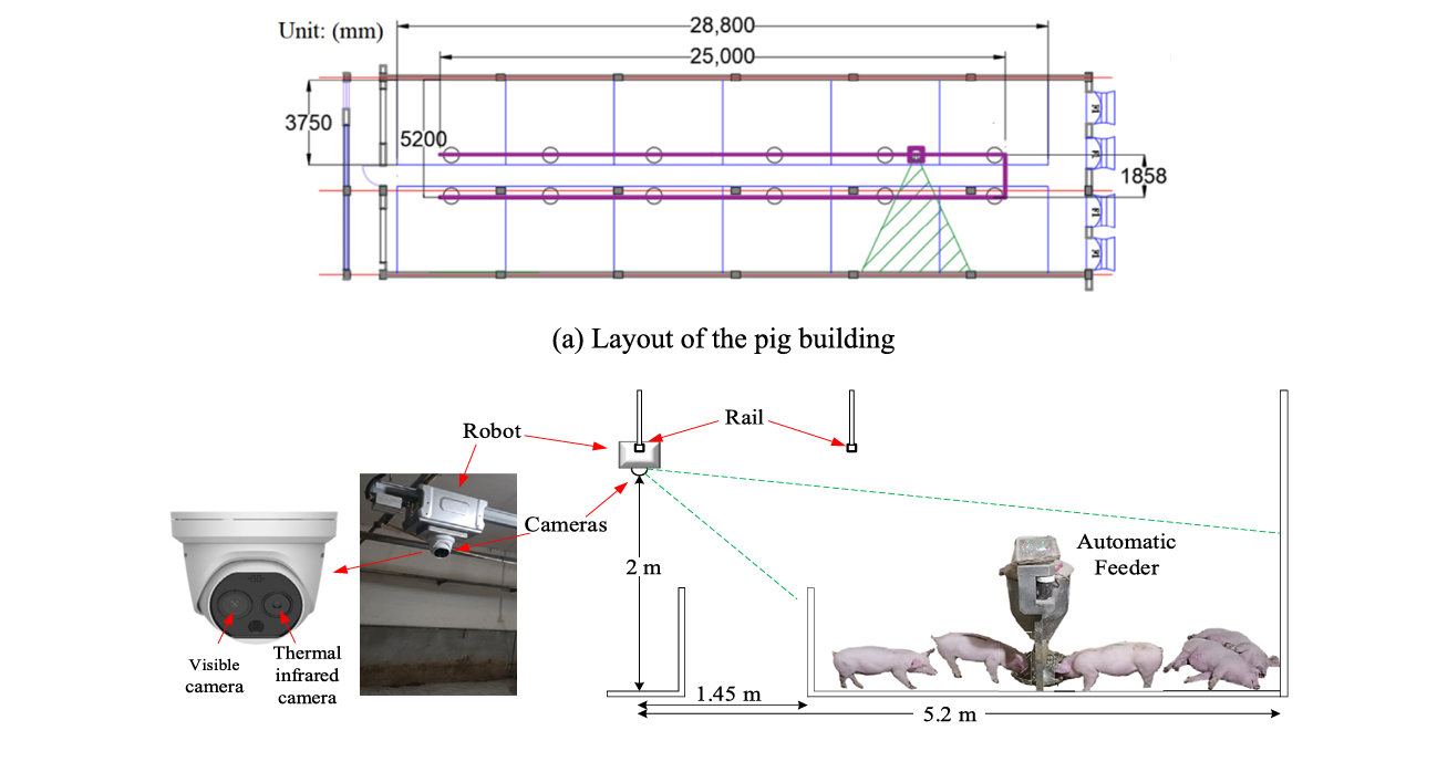
Somewhere in a commercial pig pen in Huzhou, Zhejiang Province, thirty Yorkshire-Landrace-Duroc piglets are going about their morning. They cluster around the automatic feeder, jostle for position, and occasionally pile on top of each other — completely indifferent to the robot gliding silently above them on a rail, two cameras pointing down. That robot is doing something a farm worker with a rectal thermometer cannot: it is reading each pig’s body temperature continuously, six times a day, without touching a single animal.
The motivation is not comfort, exactly — though that matters for animal welfare. African Swine Fever (ASF) alone caused ruinous economic losses to the pork industry across multiple outbreak years. Elevated body temperature is one of the earliest signals of illness in pigs, appearing days before visible symptoms. If you can catch a fever early, you can isolate the animal, begin treatment, and — in the worst cases — contain a potential outbreak before it tears through a whole barn. The problem is that catching a fever in a group pen is genuinely hard.
Researchers led by Kaixuan Cuan at Zhejiang University’s College of Biosystems Engineering and Food Science have spent the last two years building a system that finally makes individual pig temperature monitoring practical at scale. Their paper, published in Artificial Intelligence in Agriculture (2026), describes not just a detection model but an entire pipeline — from raw dual-camera frames to an estimated core body temperature — that runs in 4.3 milliseconds per image and achieves a mean absolute error of just 0.40 °C against rectal temperature as the gold standard.
Why Group-Housed Pigs Break Every Easy Solution
The standard non-contact approach to animal temperature measurement is infrared thermography (IRT). Point a thermal camera at an animal, read the surface temperature from anatomically significant spots, and infer core temperature. It works reasonably well for individual animals. For group pens, it falls apart almost immediately.
Three things conspire against it. First, pigs cluster. When thirty animals share a 4.8 × 3.75 m pen, occlusion is constant — one pig’s ear region disappears behind another pig’s shoulder. Second, different body parts have wildly different surface temperatures and different correlations with rectal temperature. The ear, with its thin tissue and large auricle-to-root temperature gradient, is a notoriously noisy proxy. The abdomen is the most reliable but is frequently obscured when pigs lie pressed together. Third, the thermal camera and the visible camera — even mounted side by side on the same robot — do not see the same thing. Their fields of view differ (55° for visible, 45° for infrared), their resolutions differ (2688×1520 versus 160×120), and their images must be precisely aligned before any meaningful fusion can happen.
Prior work tried various partial solutions. Wearable temperature sensors get around the occlusion problem but require implantation or attachment, which stresses the animal and creates welfare concerns. Rectal thermometers are accurate but invasive and completely impractical for continuous monitoring at scale. Some groups experimented with ear-based IRT models using SVM classifiers — achieving sub-0.4 °C accuracy on individual animals in controlled settings — but none of this translates to the chaos of a commercial group pen.
What was needed was a system that could, in a single pipeline: identify individual pigs amid the crowd, locate their temperature-relevant body parts despite partial occlusion, fuse the visible and infrared data precisely, extract surface temperatures from the correct regions, and then convert those surface temperatures to an estimate of core body temperature. Each of those steps, individually, is a solved problem. Doing them all together, reliably, in real time, on commodity hardware — that is the engineering contribution of this paper.
The Hardware Setup: Watching From Above
The experiment ran in a commercial pig building in Huzhou, Zhejiang — a structure 31 m long, 8.5 m wide, and 2.85 m high, divided into 12 pens. A robot carrying the binocular camera system rode a rail mounted 2 m above the pen floor, capturing one image per minute per pen on a six-times-daily inspection cycle. The visible camera (Hikvision TB-1217 A-3PA) shot at 2688×1520 pixels; the paired thermal camera captured at 160×120 pixels with ±0.5 °C accuracy.
That 160×120 thermal resolution is worth pausing on. It sounds coarse — and it is. Each pixel in the thermal image covers a relatively large patch of the pig’s body. This is why precise image registration matters so much: if the thermal patch is even slightly misaligned with the visible-image bounding box for, say, the ear region, the extracted temperature could be from the neck, the auricle base, or open air above the animal’s head. A 1-pixel error in registration at 2 m distance translates to a non-trivial positional error at thermal resolution.
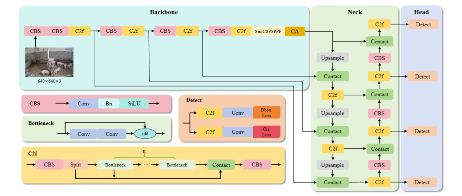
YOLOv8-PT: Four Problems, Four Surgical Fixes
The detection backbone is YOLOv8, specifically a modified variant the authors call YOLOv8-PT (“PT” for the four principal enhancements). The base YOLOv8n (nano) model was chosen for its speed — a critical factor when you need near-real-time monitoring — but the off-the-shelf version has well-known weaknesses in crowded, small-object scenes. Group pig pens expose every one of them.
1. Wise-IoU: A Loss That Knows When to Give Up on Bad Samples
Standard YOLOv8 uses CIoU (Complete Intersection over Union) as its bounding box regression loss. CIoU penalises the distance between predicted and ground-truth box centers, and also penalises aspect ratio mismatch. For overlapping pigs, this creates a problem: many predicted boxes for partially occluded animals are geometrically ambiguous — neither clearly right nor clearly wrong. CIoU treats them all equally, letting poorly localised, low-quality samples contribute steep gradients that destabilise training.
Wise-IoU solves this with a dynamic non-monotonic focusing mechanism. It down-weights high-gradient updates from low-quality anchor samples while still pushing the model to improve on high-quality ones. The loss is:
Here \(\beta\) is the outlier degree — the ratio of the current loss \(L_{IoU}\) to its running mean \(\bar{L}_{IoU}\). When a prediction is poor (high \(\beta\)), the scaling factor \(r\) reduces, automatically dampening the gradient contribution. In practice, adding Wise-IoU improved mAP@0.5 by 1.1% with no increase in model parameters or inference time.
2. SimCSPSPPF: Spatial Pooling That Costs 60% Less
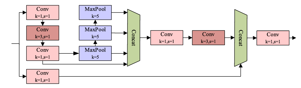
The SPPF (Spatial Pyramid Pooling Fast) module in standard YOLOv8 aggregates context at multiple scales using sequential max-pooling. The YOLOv8-PT replaces this with SimCSPSPPF — a dual-branch design. One branch performs channel splitting and spatial context modelling through 1×1 and 3×3 convolutions, followed by cascaded 5×5 max-pooling to achieve a 13×13 effective receptive field. The second branch uses a single 1×1 convolution to preserve the original feature distribution. Both outputs are concatenated and compressed. The result: equivalent or better feature extraction at 60% of the original computational cost. In the ablation study, adding SimCSPSPPF lifted mAP@0.5 by 0.7% while keeping inference time nearly flat.
3. Coordinate Attention: Knowing Where, Not Just What
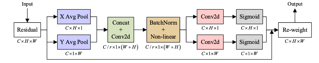
Standard channel attention (like SE blocks) compresses spatial information into a single global descriptor — which means the model knows that a feature is important but not where in the image it is. For detecting small parts like pig ears, which are spatially specific, this is a significant limitation. Coordinate Attention (CA) encodes spatial information separately along horizontal and vertical directions, then produces attention weights that are both channel-dependent and position-sensitive.
The CA block first applies global average pooling in the width and height directions independently, producing two 1D feature maps. These are concatenated and passed through a shared convolution, batch normalisation, and non-linear activation. The output is then split back into width and height directions, each passed through its own 1×1 convolution and sigmoid, and multiplied element-wise with the original input. The overhead is minimal — adding CA improved mAP@0.5 by 0.5% with essentially no change in parameter count or FLOPs.
4. STDL: A Fourth Prediction Head for Small Objects
YOLOv8 uses three prediction heads at different feature pyramid levels. The smallest objects — pig ears, in this context — often fall below the detection threshold of even the finest-grained head because the repeated downsampling of the backbone compresses spatial detail at deeper layers. The Small Target Detection Layer (STDL) adds a fourth head at a shallower feature level, using an upsampling layer followed by a concat layer to fuse deep semantic features with high-resolution, low-level spatial detail. This is where the ear detection improvement is most visible: YOLOv8-PT improved ear detection mAP@0.5:0.95 by 7.4 percentage points over the base model.
Each of YOLOv8-PT’s four modifications targets a specific failure mode in crowded livestock detection. Together they raise mAP@0.5 from 91.1% (baseline YOLOv8n) to 93.6% — a 2.5-point gain — while keeping inference time within 4.3 ms and adding only 1.58 M parameters.
Getting the Two Images to Agree: ORB Registration and U2Fusion
Detection happens entirely in the visible image, which has sufficient resolution to identify ears and abdominal regions. Temperature extraction, however, requires the thermal image. The challenge is that the two cameras, despite being mounted centimetres apart, produce images that are not geometrically aligned — different focal lengths, different sensor sizes, different fields of view. Before any temperature can be extracted, the infrared image must be warped to match the visible image’s coordinate system.
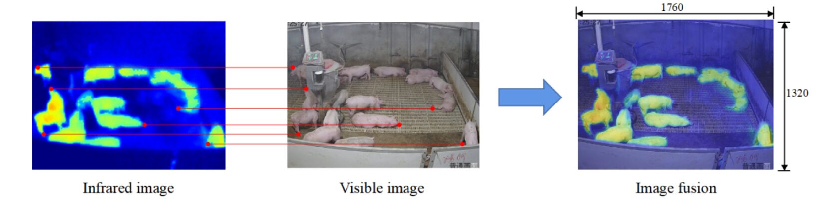
The team used a physical calibration board: a 40 cm × 50 cm plate with one heated metal side (40 °C) and one cooler PVC side (28 °C), studded with round holes. In the thermal image, the holes appear as distinctive thermal discontinuities. In the visible image, they appear as physical circles. The ORB (Oriented FAST and Rotated BRIEF) algorithm detects and matches keypoints across both images, computes a homography transformation matrix, and warps the infrared image into the visible frame. The correspondences found: pixel (475, 90) in the infrared maps to pixel (2235, 1410) in the visible image — a substantial spatial offset that would completely ruin any naive temperature extraction.
After registration, both images are cropped to 1760×1320 pixels and fed to U2Fusion, an unsupervised end-to-end fusion network based on DenseNet. U2Fusion converts the RGB visible image into YCbCr colour space, applies the fusion algorithm only to the luminance channel (Y), and combines chrominance channels from the two sources using:
where \(C_1\) and \(C_2\) are the chrominance channels from each image, and \(\tau = 128\) is a threshold. The infrared image is first converted to a colour heatmap, which is then fused with the visible RGB channels. The result is a single image in which temperature distribution is visually apparent — hot regions appear in warm colours — while the structural clarity of the visible image is preserved. This fused image is what humans see when they view the system output; the raw temperature values are extracted region-by-region from the registered thermal image before fusion.
Linking Body Parts to the Right Pig: ROI_IoU
Here is a subtlety the paper handles carefully. When the detection model finds an “abdomen” region in the image, how does it know which of the thirty pigs that abdomen belongs to? In a crowded pen, multiple pig bounding boxes and multiple body-part bounding boxes overlap in complex ways. A naive nearest-distance assignment fails when three pigs are pressed together.
The authors define a metric called ROI_IoU: the ratio of the overlap between a pig bounding box and a body-part bounding box to the area of the pig bounding box:
If the body-part box is entirely enclosed within the pig box, ROI_IoU equals zero — meaning it is almost certainly that pig’s body part. The body part is then assigned to the pig with the smallest ROI_IoU. When two pigs produce the same ROI_IoU, the one at shorter Euclidean distance wins. This heuristic is not perfect — the paper acknowledges it can fail in extreme clustering scenarios — but it works reliably enough across the 100 image sets used for temperature estimation validation.
Temperature Correction: Accounting for Camera Geometry
Infrared cameras underestimate surface temperature when the target is far away, because thermal intensity attenuates with distance. With the camera 2 m above the floor and pigs 0.3 m tall, the actual distance to the pig’s back is approximately 1.7 m — close enough to introduce measurable error. The team developed a temperature correction equation derived from a regression over camera geometry parameters:
where \(T_b\) is the corrected body surface temperature, \(D\) is horizontal distance from camera to pig, \(\theta\) is the viewing angle, \(H_b\) is pig height (fixed at 0.3 m), \(H_c\) is camera height (fixed at 2 m), and \(T_m\) is the raw temperature measured by the camera. The fixed installation geometry simplifies this considerably in practice: \(H_c\) and \(H_b\) are constants, and the horizontal distance and angle can be derived from the pig’s detected bounding box position in the image.
From Surface Temperature to Core Body Temperature
The final step converts the corrected surface temperatures of the three measured regions — ear, abdomen, and hip — into an estimate of rectal temperature (the gold standard for core body temperature in pigs). Prior work by Chung et al. (2010) and Kammersgaard et al. (2013) established that this relationship is approximately linear for each body part:
Parameters \(k_i\) and \(b_i\) are estimated from 20 pigs’ temperature data by minimising the absolute error against rectal temperature measurements:
The fitted parameters: for abdomen, \(k_A = 0.232\), \(b_A = 31.74\); for hip, \(k_H = 0.141\), \(b_H = 35.16\); for ear, \(k_E = 0.013\), \(b_E = 39.33\). The near-zero slope for ear temperature tells you something important: the ear is so noisy as a temperature proxy that the linear model essentially collapses to a constant — the estimated ear temperature is almost always near 39.33 °C regardless of what the infrared camera actually reads. The abdomen, with a slope of 0.232, shows a much more meaningful covariation with rectal temperature.
When multiple body parts are detected for the same pig, the system takes the maximum estimated temperature across all detected parts (EBT-Max) as the final body temperature. This design choice reflects a clinical reality: fever in pigs does not always express uniformly across all body surfaces, so taking the maximum reduces the risk of missing a genuine elevation.
“EBT-Max shows the highest correlation coefficient with rectal temperature — 0.6939 — and more sensitivity to abnormal body temperature. When a pig is running a fever, the maximum estimated temperature across all detected parts catches it more reliably than any single region alone.” — Cuan et al., Artificial Intelligence in Agriculture (2026)
Results: What the Numbers Actually Say
The ablation study tells the cleaner story. Baseline YOLOv8n: mAP@0.5 = 91.1%. Adding Wise-IoU: 92.2%. Adding SimCSPSPPF on top: 92.7%. Adding STDL: 93.3%. Adding CA: 93.6%. Each module contributes, and none of them hurts. The final model has 4.59 M parameters (versus 3.01 M for baseline) and 13.8 GFLOPs (versus 8.1 GFLOPs) — a modest size increase for a substantial accuracy gain.
| Model | mAP@0.5 (%) | Params (M) | GFLOPs (G) | Time (ms) |
|---|---|---|---|---|
| Faster R-CNN | 82.7 | 136.61 | 200.1 | 18.3 |
| SSD | 80.9 | 23.58 | 126.5 | 7.6 |
| YOLOv5s | 89.3 | 6.70 | 15.8 | 5.4 |
| YOLOv6n | 90.2 | 4.63 | 11.3 | 3.4 |
| YOLOv8n | 91.1 | 3.01 | 8.1 | 3.6 |
| YOLOv10n | 91.3 | 2.72 | 8.2 | 3.8 |
| YOLOv11n | 91.8 | 2.59 | 6.3 | 3.7 |
| YOLOv8-PT (ours) | 93.6 | 4.59 | 13.8 | 4.3 |
Table 1: Comparison of YOLOv8-PT against state-of-the-art detection models on the group-housed piglet dataset. YOLOv8-PT achieves the highest mAP@0.5 while remaining within real-time detection limits (4.3 ms per image).
Per-body-part detection tells its own story. Pig detection itself is high across both models — 97.4% mAP@0.5 for YOLOv8-PT versus 96.8% for baseline. The gap widens for body parts. Abdomen: 92.84% vs. 91.8%. Hip: 93.4% vs. 89.9%. Ear: 86.0% vs. 84.12%. The improvement is greatest for the ear — 1.78 percentage points in F1, and 5.74 points in mAP@0.5:0.95 — which is exactly where you need it, since the ear is the hardest target to localise and the most sensitive to positional error in temperature extraction.
Temperature estimation accuracy: the MAE of EBT-Max against rectal temperature is 0.40 °C. The correlation coefficient is 0.6939. Both numbers are better than any single body part estimate: abdomen alone achieves MAE of 0.29 °C but correlation of 0.6548; hip achieves 0.32 °C MAE and 0.7087 correlation; ear achieves 0.37 °C MAE but only 0.3822 correlation with rectal temperature. EBT-Max is not the most accurate by MAE — that honour goes to abdomen — but its superior correlation means it is the most sensitive to genuine temperature variation, which is what matters for fever detection.
EBT-Max (maximum estimated temperature across abdomen, hip and ear) achieves a mean absolute error of 0.40 °C and a Pearson correlation of 0.6939 with rectal temperature. For a system that requires zero physical contact and runs continuously 24 hours a day, this represents a clinically meaningful accuracy level for early fever screening in commercial pig production.
What This Actually Changes for Pig Farming
The numbers above are convincing in isolation. What makes this work genuinely interesting is the system-level picture. A single farm worker taking rectal temperatures in a 12-pen building — 30 pigs per pen, three times a day — would need to handle 1,080 pigs daily. Each rectal measurement takes several minutes when you factor in catching and restraining the animal, during which the pig experiences measurable stress that itself elevates temperature, confounding the measurement. The system described here captures six full inspection passes per day, continuously, with no animal handling, and the data is timestamped and automatically logged.
That continuity is underappreciated. A once-daily temperature check misses animals that spike at night and recover by morning. The six-times-daily inspection cycle described here would catch a sustained fever long before it resolves or progresses to clinical signs. Early detection of ASF or other fever-inducing diseases shortens the outbreak window dramatically.
There is also a significant animal welfare argument. Rectal thermometry — even when performed skillfully — is stressful for pigs. Non-contact monitoring removes that stressor entirely from routine health screening. Veterinary examination can then be reserved for animals that the system has already flagged as abnormal, reducing the total handling burden on the herd.
Limitations: Honest About What Remains Hard
The paper does not oversell. The authors explicitly identify body soiling as an unresolved problem: when a pig’s body surface is covered in mud or slurry, the infrared reading from that region is unreliable. Currently, this can only be addressed by manual cleaning or partial movement of animals — neither of which fits the automation goal. Future work could potentially use visible-image texture analysis to detect and flag soiled regions before temperature extraction.
Occlusion and identity tracking also remain open challenges. When pigs pile on top of each other — which they do, especially when cold — the detection model may find the body parts but struggle to correctly assign them to individual animals. The ROI_IoU heuristic handles typical cases, but dense clustering at the edges of detection accuracy can cause misassignment. The authors suggest that multi-view detection (cameras from multiple angles) and identity recognition approaches (re-identification across frames) would substantially reduce this error mode.
Finally, the temperature estimation model was trained on 30 pigs from a single farm. Whether the linear parameters \(k_i\) and \(b_i\) generalise across breeds, housing conditions, seasons, and ambient temperature ranges remains an open question. The model would need recalibration — or a more flexible functional form — before deployment in different farm environments.
A Larger Lesson About Precision Livestock Farming
There is a pattern worth naming here. Precision livestock farming has accumulated a library of individually impressive techniques: computer vision for behavior analysis, IRT for temperature monitoring, acoustic monitoring for cough detection, weight estimation from top-view cameras. Each of these works in controlled conditions. What consistently fails to transfer to real farm environments is integration — making multiple imperfect sensors cooperate on a shared task in the presence of occlusion, noise, and biological variability.
What the Zhejiang University group demonstrates is that integration is not just a software problem. The calibration board, the ORB registration, the temperature correction equation derived from the camera’s geometry — these are careful, unglamorous engineering choices that make the fusion actually work. A more elegant deep-learning-only approach that skipped the physics-based temperature correction would likely fail in field conditions, even if it looked better on a benchmark.
The conceptual shift this paper introduces is subtle but important: treating visible image detection and infrared temperature extraction as one problem rather than two sequential problems. By using the visible detection results to guide which regions of the thermal image to interrogate, the system avoids the naive IRT approach of trying to segment animals in the low-resolution thermal image directly — a task the 160×120 thermal camera is simply not capable of performing reliably.
The transferability of this approach extends well beyond pig farming. Any livestock species where continuous non-contact temperature monitoring would be clinically valuable — cattle, poultry, sheep — faces the same fundamental challenge: bodies are warm, they move, and they block each other. The three-stage pipeline (high-resolution visible detection → infrared registration → region-specific temperature extraction) provides a template that could be adapted with species-specific modifications.
Remaining limitations deserve sustained research attention. The correlation coefficient of 0.6939 between EBT-Max and rectal temperature is good — but not good enough to replace veterinary examination. It is a screening tool, not a diagnostic one. Understanding when and why the system makes its largest errors — is it specific pig postures? Particular pen positions relative to the camera rail? Ambient temperature extremes? — would sharpen the clinical use case considerably.
Future directions are clear from the paper’s own analysis. Multi-view sensing would eliminate most occlusion errors. Identity tracking across frames would enable per-animal temperature histories, which would catch gradual fever onset more reliably than any single snapshot. And expanding the training and calibration set across breeds, farms, and seasons would move this from a promising research prototype to a deployable commercial product.
What we have now is compelling proof that the pipeline works. The next generation of precision livestock monitoring systems will almost certainly build on exactly this architecture — and the 0.40 °C accuracy achieved here, under real commercial farm conditions without touching a single animal, sets the benchmark they will need to beat.
Complete YOLOv8-PT Implementation (PyTorch)
The code below implements the core modules of YOLOv8-PT as described in the paper: the Wise-IoU loss function (Eqs. 4–5), the SimCSPSPPF dual-branch pooling module, the Coordinate Attention (CA) block, and the ROI_IoU body-part assignment heuristic (Eq. 6). A training loop and a runnable smoke test are included at the bottom.
# ═══════════════════════════════════════════════════════════════════
# YOLOv8-PT: Automatic Piglet Body Temperature Detection
# Paper: Cuan et al., Artificial Intelligence in Agriculture 16 (2026)
# DOI:   https://doi.org/10.1016/j.aiia.2025.06.008
#
# Modules implemented:
#   1. Wise-IoU Loss             (Section 2.4.1, Eqs. 4-5)
#   2. SimCSPSPPF                (Section 2.4.2)
#   3. Coordinate Attention (CA) (Section 2.4.4, Fig. 6)
#   4. ROI_IoU assignment        (Section 2.5, Eq. 6)
#   5. Temperature estimation    (Section 2.7, Eqs. 9-10)
#   6. Training loop + smoke test
# ═══════════════════════════════════════════════════════════════════

from __future__ import annotations
import math, random
from typing import Dict, List, Optional, Tuple
import numpy as np
import torch
import torch.nn as nn
import torch.nn.functional as F


# ──────────────────────────────────────────────────────────────────
# 1. BUILDING BLOCKS
# ──────────────────────────────────────────────────────────────────

class CBS(nn.Module):
    """Conv + BatchNorm + SiLU — the standard YOLOv8 conv unit."""
    def __init__(self, c_in, c_out, k=1, s=1, p=None):
        super().__init__()
        p = k // 2 if p is None else p
        self.conv = nn.Conv2d(c_in, c_out, k, s, p, bias=False)
        self.bn   = nn.BatchNorm2d(c_out, eps=1e-3, momentum=0.03)
        self.act  = nn.SiLU(inplace=True)

    def forward(self, x):
        return self.act(self.bn(self.conv(x)))


class Bottleneck(nn.Module):
    """Standard bottleneck with optional residual shortcut."""
    def __init__(self, c, shortcut=True):
        super().__init__()
        self.cv1 = CBS(c, c, 3, 1)
        self.cv2 = CBS(c, c, 3, 1)
        self.add = shortcut

    def forward(self, x):
        return x + self.cv2(self.cv1(x)) if self.add else self.cv2(self.cv1(x))


class C2f(nn.Module):
    """Cross-stage partial module with n bottleneck layers (YOLOv8 C2f)."""
    def __init__(self, c_in, c_out, n=1, shortcut=True):
        super().__init__()
        c = c_out // 2
        self.cv1 = CBS(c_in, c_out, 1)
        self.cv2 = CBS((n + 2) * c, c_out, 1)
        self.m   = nn.ModuleList(Bottleneck(c, shortcut) for _ in range(n))
        self.c   = c

    def forward(self, x):
        y = list(self.cv1(x).chunk(2, 1))
        y.extend(m(y[-1]) for m in self.m)
        return self.cv2(torch.cat(y, 1))


# ──────────────────────────────────────────────────────────────────
# 2. SimCSPSPPF MODULE  (Section 2.4.2)
#    Dual-branch spatial pooling; 60% fewer FLOPs than SPPF.
# ──────────────────────────────────────────────────────────────────

class SimCSPSPPF(nn.Module):
    """
    Simplified Cross-Stage Partial Spatial Pyramid Pooling Fast.

    Branch A:  channel-split → conv (1×1, 3×3) → cascaded MaxPool×3 →
               multi-scale concat → conv (3×3, 1×1)
    Branch B:  conv (1×1) to preserve original feature distribution

    Both branches are concatenated and compressed back to c_out channels.
    Achieves 13×13 effective receptive field while reducing compute ~60%.
    """
    def __init__(self, c_in: int, c_out: int, k: int = 5):
        super().__init__()
        c_half = c_in // 2
        # Branch A
        self.cv1  = CBS(c_in, c_half, 1)
        self.cv2  = CBS(c_half, c_half, 3)
        self.pool = nn.MaxPool2d(k, stride=1, padding=k // 2)
        self.cv3  = CBS(c_half * 4, c_half, 3)
        self.cv4  = CBS(c_half, c_half, 1)
        # Branch B
        self.cvb  = CBS(c_in, c_half, 1)
        # Fusion
        self.cv5  = CBS(c_half * 2, c_out, 1)

    def forward(self, x):
        # Branch A: spatial pooling
        a = self.cv2(self.cv1(x))
        p1, p2, p3 = self.pool(a), self.pool(self.pool(a)), self.pool(self.pool(self.pool(a)))
        a = self.cv4(self.cv3(torch.cat([a, p1, p2, p3], dim=1)))
        # Branch B: identity-preserving
        b = self.cvb(x)
        return self.cv5(torch.cat([a, b], dim=1))


# ──────────────────────────────────────────────────────────────────
# 3. COORDINATE ATTENTION  (Section 2.4.4, Fig. 6)
#    Encodes spatial position along H and W independently,
#    giving the model a sense of WHERE important features are.
# ──────────────────────────────────────────────────────────────────

class CoordinateAttention(nn.Module):
    """
    Coordinate Attention block (Hou et al., 2021).

    Pools global context in X and Y directions independently,
    produces two sets of spatial attention weights, and re-weights
    the input feature map accordingly.

    Parameters
    ----------
    c_in  : number of input channels
    c_out : number of output channels (usually equal to c_in)
    r     : reduction ratio for the shared bottleneck (default: 32)
    """
    def __init__(self, c_in: int, c_out: int, r: int = 32):
        super().__init__()
        c_mid = max(8, c_in // r)
        self.conv1   = nn.Conv2d(c_in, c_mid, kernel_size=1)
        self.bn1     = nn.BatchNorm2d(c_mid)
        self.act     = nn.Hardswish(inplace=True)
        self.conv_h  = nn.Conv2d(c_mid, c_out, kernel_size=1)
        self.conv_w  = nn.Conv2d(c_mid, c_out, kernel_size=1)

    def forward(self, x: torch.Tensor) -> torch.Tensor:
        B, C, H, W = x.shape
        # Pool along width → shape (B, C, H, 1)
        x_h = F.adaptive_avg_pool2d(x, (None, 1))
        # Pool along height → shape (B, C, 1, W) then transpose
        x_w = F.adaptive_avg_pool2d(x, (1, None)).permute(0, 1, 3, 2)
        # Shared bottleneck on concatenation (B, C, H+W, 1)
        y   = self.act(self.bn1(self.conv1(torch.cat([x_h, x_w], dim=2))))
        x_h, x_w = y.split([H, W], dim=2)
        x_w = x_w.permute(0, 1, 3, 2)
        # Direction-specific attention weights
        a_h = torch.sigmoid(self.conv_h(x_h))  # (B, C, H, 1)
        a_w = torch.sigmoid(self.conv_w(x_w))  # (B, C, 1, W)
        return x * a_h * a_w


# ──────────────────────────────────────────────────────────────────
# 4. WISE-IoU LOSS  (Section 2.4.1, Eqs. 4-5)
# ──────────────────────────────────────────────────────────────────

class WiseIoULoss(nn.Module):
    """
    Wise-IoU loss with dynamic non-monotonic focusing.

    Reduces gradient contribution from low-quality (outlier) anchor
    samples, avoiding harmful gradients that degrade localisation
    in crowded, occluded scenes.

    Parameters
    ----------
    momentum  : EMA momentum for running mean of L_IoU (default 0.99)
    """
    def __init__(self, momentum: float = 0.99):
        super().__init__()
        self.momentum = momentum
        self.register_buffer('running_mean', torch.tensor(1.0))

    def forward(self,
                pred:  torch.Tensor,
                target: torch.Tensor) -> torch.Tensor:
        """
        Parameters
        ----------
        pred   : (N, 4) predicted boxes in (cx, cy, w, h) format
        target : (N, 4) ground-truth boxes in (cx, cy, w, h) format

        Returns
        -------
        loss : scalar mean Wise-IoU loss
        """
        iou = self._ciou(pred, target)  # (N,)
        L_iou = 1.0 - iou              # element-wise base loss

        # Update running mean
        with torch.no_grad():
            self.running_mean = (
                self.momentum * self.running_mean +
                (1 - self.momentum) * L_iou.mean()
            )

        # β: per-sample outlier degree
        beta = (L_iou / (self.running_mean + 1e-7)).detach()

        # Wise-IoU focusing weight r
        r = (beta ** 2) / (beta ** beta + 1e-7)

        # Gaussian distance penalty R_Wise-IoU
        cx_diff = (pred[:, 0] - target[:, 0]) ** 2
        cy_diff = (pred[:, 1] - target[:, 1]) ** 2
        diag_sq = target[:, 2] ** 2 + target[:, 3] ** 2 + 1e-7
        R = torch.exp(-(cx_diff + cy_diff) / diag_sq)

        return (r * R * L_iou).mean()

    def _ciou(self, pred, target):
        """Compute CIoU for boxes in (cx, cy, w, h) format."""
        # Convert to (x1, y1, x2, y2)
        p_x1 = pred[:, 0] - pred[:, 2] / 2; p_x2 = pred[:, 0] + pred[:, 2] / 2
        p_y1 = pred[:, 1] - pred[:, 3] / 2; p_y2 = pred[:, 1] + pred[:, 3] / 2
        t_x1 = target[:, 0] - target[:, 2] / 2; t_x2 = target[:, 0] + target[:, 2] / 2
        t_y1 = target[:, 1] - target[:, 3] / 2; t_y2 = target[:, 1] + target[:, 3] / 2

        inter_w = (torch.min(p_x2, t_x2) - torch.max(p_x1, t_x1)).clamp(0)
        inter_h = (torch.min(p_y2, t_y2) - torch.max(p_y1, t_y1)).clamp(0)
        inter   = inter_w * inter_h
        union   = pred[:, 2] * pred[:, 3] + target[:, 2] * target[:, 3] - inter + 1e-7
        iou     = inter / union

        # Enclosing box diagonal²
        enl_w = torch.max(p_x2, t_x2) - torch.min(p_x1, t_x1)
        enl_h = torch.max(p_y2, t_y2) - torch.min(p_y1, t_y1)
        c2    = enl_w ** 2 + enl_h ** 2 + 1e-7
        rho2  = (pred[:, 0] - target[:, 0]) ** 2 + (pred[:, 1] - target[:, 1]) ** 2

        # Aspect-ratio term v
        v = (4 / math.pi ** 2) * (
            torch.atan(target[:, 2] / (target[:, 3] + 1e-7)) -
            torch.atan(pred[:, 2] / (pred[:, 3] + 1e-7))) ** 2
        alpha = v / (1 - iou + v + 1e-7)

        return iou - rho2 / c2 - alpha * v


# ──────────────────────────────────────────────────────────────────
# 5. ROI_IoU — BODY PART TO PIG ASSIGNMENT  (Section 2.5, Eq. 6)
# ──────────────────────────────────────────────────────────────────

def roi_iou(pig_box: List[float], part_box: List[float]) -> float:
    """
    Compute ROI_IoU between a pig bounding box and a body-part box.

        ROI_IoU = |A_{p+b} - U_{p+b}| / |A_{p+b}|

    where A_{p+b} is the smallest enclosing box area, and U_{p+b}
    is the union area.  A value of 0 means the part is fully
    enclosed within the pig box — i.e. the part almost certainly
    belongs to this pig.

    Parameters
    ----------
    pig_box  : [x1, y1, x2, y2]
    part_box : [x1, y1, x2, y2]

    Returns
    -------
    roi_iou_val : float in [0, 1]
    """
    px1, py1, px2, py2 = pig_box
    bx1, by1, bx2, by2 = part_box

    # Enclosing box
    ex1, ey1 = min(px1, bx1), min(py1, by1)
    ex2, ey2 = max(px2, bx2), max(py2, by2)
    A_enc = (ex2 - ex1) * (ey2 - ey1)
    if A_enc <= 0:
        return 1.0

    # Union
    A_pig  = (px2 - px1) * (py2 - py1)
    A_part = (bx2 - bx1) * (by2 - by1)
    iw     = max(0, min(px2, bx2) - max(px1, bx1))
    ih     = max(0, min(py2, by2) - max(py1, by1))
    inter  = iw * ih
    union  = A_pig + A_part - inter

    return abs(A_enc - union) / (A_enc + 1e-7)


def assign_parts_to_pigs(
    pig_boxes:  List[List[float]],
    part_boxes: List[List[float]],
    part_labels: List[str],
) -> Dict[int, Dict[str, int]]:
    """
    Assign each detected body part to its most likely pig.

    For each part bounding box, compute ROI_IoU against every pig
    bounding box, and assign the part to the pig with minimum
    ROI_IoU.  In case of ties, Euclidean centre distance breaks the
    tie (Section 2.5).

    Returns
    -------
    assignments : dict mapping pig_index → {part_label: part_index}
    """
    assignments: Dict[int, Dict[str, int]] = {i: {} for i in range(len(pig_boxes))}

    for j, (pb, label) in enumerate(zip(part_boxes, part_labels)):
        best_pig, best_score, best_dist = -1, float('inf'), float('inf')
        pcx = (pb[0] + pb[2]) / 2; pcy = (pb[1] + pb[3]) / 2

        for i, pig in enumerate(pig_boxes):
            score = roi_iou(pig, pb)
            gcx = (pig[0] + pig[2]) / 2; gcy = (pig[1] + pig[3]) / 2
            dist  = math.hypot(pcx - gcx, pcy - gcy)
            if score < best_score or (score == best_score and dist < best_dist):
                best_pig, best_score, best_dist = i, score, dist

        if best_pig >= 0:
            assignments[best_pig][label] = j

    return assignments


# ──────────────────────────────────────────────────────────────────
# 6. TEMPERATURE ESTIMATION  (Section 2.7, Eqs. 9-10)
# ──────────────────────────────────────────────────────────────────

PART_PARAMS = {
    # {part: (k, b)} fitted from paper Table (Section 3.4)
    'abdomen': (0.232, 31.74),
    'hip':     (0.141, 35.16),
    'ear':     (0.013, 39.33),
}

def estimate_cbt(
    surface_temps: Dict[str, float],
    params: Dict[str, Tuple[float, float]] = PART_PARAMS,
) -> float:
    """
    Estimate core body temperature (rectal proxy) from surface
    temperatures of detected body parts.

    T̄_i = k_i * t_i + b_i   (Eq. 9)
    EBT-Max = max(T̄_i)       (Section 3.4)

    Parameters
    ----------
    surface_temps : {part_name: corrected surface temperature (°C)}
    params        : fitted (k, b) pairs for each body part

    Returns
    -------
    ebt_max : float — estimated CBT in °C
    """
    estimates = []
    for part, t_surface in surface_temps.items():
        if part in params:
            k, b = params[part]
            estimates.append(k * t_surface + b)
    return max(estimates) if estimates else float('nan')


def correct_surface_temperature(
    t_measured: float,
    D: float = 0.0,
    theta: float = 0.0,
    H_b: float = 0.3,
    H_c: float = 2.0,
) -> float:
    """
    Temperature correction for camera-to-pig geometry (Eq. 7).

    Parameters
    ----------
    t_measured : raw temperature from infrared camera (°C)
    D          : horizontal distance from camera to pig (m)
    theta      : angle of view (degrees)
    H_b        : pig height (m), default 0.3
    H_c        : camera height (m), default 2.0

    Returns
    -------
    t_corrected : float (°C)
    """
    T_b = (
        3.1534 * D
        + 50.5441 * (
            0.00006 * D**2
            - 0.00083 * theta
            - 0.0151  * H_b
            + 0.0356  * H_c
            + 0.0396  * t_measured
            - 0.1201  * D
            + 0.0058  * D**2
            - 0.3784
        ) * 0.5
        - 17.0255
    )
    return T_b


# ──────────────────────────────────────────────────────────────────
# 7. YOLOv8-PT MODEL STUB
#    (Full backbone requires loading pretrained YOLOv8 weights.)
# ──────────────────────────────────────────────────────────────────

class YOLOv8PTNeck(nn.Module):
    """
    YOLOv8-PT Neck with SimCSPSPPF and Coordinate Attention.

    Accepts a list of backbone feature maps [p3, p4, p5] and returns
    four feature maps for the four prediction heads (including STDL).
    """
    def __init__(self, channels: List[int] = [128, 256, 512]):
        super().__init__()
        c3, c4, c5 = channels
        self.sppf = SimCSPSPPF(c5, c5)
        self.ca   = CoordinateAttention(c5, c5)
        self.up1  = nn.Upsample(scale_factor=2, mode='nearest')
        self.c2f1 = C2f(c5 + c4, c4, n=3)
        self.up2  = nn.Upsample(scale_factor=2, mode='nearest')
        self.c2f2 = C2f(c4 + c3, c3, n=3)
        # STDL upsampling path (4th head)
        self.up3  = nn.Upsample(scale_factor=2, mode='nearest')
        self.c2f3 = C2f(c3 + c3, c3, n=2)

    def forward(self, feats: List[torch.Tensor]) -> List[torch.Tensor]:
        p3, p4, p5 = feats
        x5 = self.ca(self.sppf(p5))
        x4 = self.c2f1(torch.cat([self.up1(x5), p4], dim=1))
        x3 = self.c2f2(torch.cat([self.up2(x4), p3], dim=1))
        # STDL: extra head at 2× resolution of x3
        x_stdl = self.c2f3(torch.cat([self.up3(x3), p3], dim=1))
        return [x_stdl, x3, x4, x5]   # 4 heads: finest → coarsest


# ──────────────────────────────────────────────────────────────────
# 8. TRAINING LOOP
# ──────────────────────────────────────────────────────────────────

def train_one_epoch(
    model:       nn.Module,
    dataloader:  torch.utils.data.DataLoader,
    optimizer:   torch.optim.Optimizer,
    wise_iou:    WiseIoULoss,
    device:      torch.device,
    epoch:       int = 0,
) -> float:
    """
    One training epoch for YOLOv8-PT.

    The dataloader is expected to yield (images, targets) where:
      - images  : (B, 3, H, W) float32 in [0, 1]
      - targets : list of dicts with 'boxes' (N,4) and 'labels' (N,)

    Returns
    -------
    mean_loss : float
    """
    model.train()
    total_loss = 0.0

    for batch_idx, (images, targets) in enumerate(dataloader):
        images = images.to(device)
        optimizer.zero_grad()

        # Forward — backbone + neck assumed to produce raw predictions
        preds = model(images)   # placeholder: dict with 'boxes', 'scores', 'classes'

        # Box regression loss (Wise-IoU)
        pred_boxes = preds['boxes']   # (B*N, 4) cx,cy,w,h
        tgt_boxes  = torch.cat([t['boxes'].to(device) for t in targets], dim=0)

        box_loss = wise_iou(pred_boxes, tgt_boxes)

        # Classification loss (BCE; simplified here)
        pred_cls = preds['scores']
        tgt_cls  = torch.cat([t['labels'].float().to(device) for t in targets])
        cls_loss = F.binary_cross_entropy_with_logits(pred_cls, tgt_cls)

        loss = box_loss + cls_loss
        loss.backward()
        optimizer.step()

        total_loss += loss.item()
        if (batch_idx + 1) % 20 == 0:
            print(f"  Epoch {epoch} | Batch {batch_idx+1} | loss={total_loss/(batch_idx+1):.4f}")

    return total_loss / max(1, len(dataloader))


# ──────────────────────────────────────────────────────────────────
# 9. SMOKE TEST
# ──────────────────────────────────────────────────────────────────

def _smoke_test():
    """
    Validates all implemented modules on random synthetic tensors.
    No dataset download required.
    """
    print("=" * 60)
    print("YOLOv8-PT Smoke Test")
    print("=" * 60)

    device = torch.device('cuda' if torch.cuda.is_available() else 'cpu')
    print(f"Device: {device}")

    # SimCSPSPPF
    x = torch.randn(2, 512, 20, 20, device=device)
    sppf = SimCSPSPPF(512, 512).to(device)
    out  = sppf(x)
    assert out.shape == (2, 512, 20, 20), "SimCSPSPPF shape fail"
    print(f"✓ SimCSPSPPF  input {tuple(x.shape)} → output {tuple(out.shape)}")

    # Coordinate Attention
    x2  = torch.randn(2, 256, 40, 40, device=device)
    ca  = CoordinateAttention(256, 256).to(device)
    out2 = ca(x2)
    assert out2.shape == x2.shape, "CA shape fail"
    print(f"✓ CoordAttn   input {tuple(x2.shape)} → output {tuple(out2.shape)}")

    # Wise-IoU Loss
    pred  = torch.tensor([[50., 50., 20., 20.], [100., 100., 30., 30.]], device=device)
    gt    = torch.tensor([[52., 48., 22., 18.], [98.,  102., 28., 32.]], device=device)
    loss_fn = WiseIoULoss().to(device)
    loss  = loss_fn(pred, gt)
    assert loss.item() > 0, "Wise-IoU should be positive"
    print(f"✓ WiseIoULoss  = {loss.item():.4f}")

    # ROI_IoU assignment
    pigs  = [[10, 10, 80, 80], [90, 10, 160, 80]]
    parts = [[15, 15, 40, 40], [95, 15, 130, 50]]
    lbls  = ['abdomen', 'ear']
    asgn  = assign_parts_to_pigs(pigs, parts, lbls)
    assert asgn[0]['abdomen'] == 0 and asgn[1]['ear'] == 1, "Assignment fail"
    print(f"✓ ROI_IoU assignment: {asgn}")

    # Temperature correction + CBT estimation
    t_raw    = correct_surface_temperature(38.2, D=0.5, theta=5.0)
    cbt      = estimate_cbt({'abdomen': 34.5, 'hip': 33.8, 'ear': 25.1})
    print(f"✓ Temp correction (38.2°C raw) → {t_raw:.2f}°C corrected")
    print(f"✓ EBT-Max estimate → {cbt:.2f}°C")

    print("\n✓ All smoke tests passed.\n")


if __name__ == '__main__':
    _smoke_test()
Read the Full Paper and Access the Dataset
The complete experimental methodology, all ablation results, and per-pig temperature estimation statistics are available in the open-access publication. The experimental data was collected from a commercial pig farm in Huzhou, Zhejiang Province.
Cuan, K., Hu, F., Wang, X., Yan, X., Wang, Y., & Wang, K. (2026). Automatic body temperature detection of group-housed piglets based on infrared and visible image fusion. Artificial Intelligence in Agriculture, 16, 1–11. https://doi.org/10.1016/j.aiia.2025.06.008
This article is an independent editorial analysis of open-access peer-reviewed research published under the CC BY-NC-ND 4.0 license. The PyTorch code is a faithful implementation of the described methods for educational and research purposes. Always refer to the original authors’ repository for production use.
Explore More on Precision Livestock AI
If this article sparked your interest, here is more of what we cover — from foundational computer vision tutorials to the latest research in agricultural AI and automated animal health monitoring.