RepVIS-GAN: Teaching a Satellite to See in the Dark by Reading the Heat It Can Already Feel
Every night, weather satellites go partially blind — their visible cameras shut off the moment the sun dips below the horizon. Researchers at Ocean University of China built a reparameterized GAN that reads three thermal infrared channels and reconstructs what the visible camera would have seen, achieving state-of-the-art accuracy on Fengyun-4A while processing all of China in under five minutes per frame.
The Fengyun-4A geostationary satellite sits above the equator at 104.7°E, scanning China’s weather every five minutes. Its visible channel at 0.65 μm delivers beautiful, high-contrast imagery of clouds, coastlines, and storm systems — but only during daylight. After sunset, that channel goes dark. You’re left with thermal infrared channels that tell you temperature but not structure. For typhoon tracking, flood monitoring, and nighttime nowcasting, that gap is operationally critical. RepVIS-GAN from Ocean University of China and the China Meteorological Administration Tornado Key Laboratory bridges that gap by learning the statistical relationship between three physically meaningful infrared channels and the visible reflectance they implicitly encode — then executing that translation fast enough for real operational use.
The Nighttime Visibility Problem and Why It’s Harder Than It Looks
At first glance, translating infrared observations into visible images sounds like a straightforward regression task. You have three input channels — surface temperature and low albedo at 3.75 μm (CH08), mid-tropospheric water vapor at 7.10 μm (CH10), and longwave window at 10.70 μm (CH12) — and you want to predict the 0.65 μm visible reflectance. Each infrared channel encodes something physically meaningful: cloud-top temperature contrasts, moisture distribution, and stable thermal structure all carry information about what clouds look like in visible light.
The difficulty is that the mapping is nonlinear, scene-dependent, and requires capturing relationships between channels, not just each channel independently. A pixel’s visible reflectance depends on whether it’s a thick cumulonimbus (high, cold, bright white), thin cirrus (cold but semi-transparent), or an ocean surface at night (warm, dark). Disentangling these scenarios requires jointly analyzing multiple spectral channels and their differences. Previous methods either ignored inter-channel differences entirely or computed them for only a subset of channel pairs. RepVIS-GAN computes all pairwise differences from all three input channels — that’s 3 pairs from 3 channels — and routes them through a purpose-built attention architecture before any encoding happens.
The second difficulty is real-time throughput. FY-4A updates its China-region scan every 5 minutes. Reconstructing a full-resolution VIS image across the 4,200 × 6,200 pixel China domain must happen faster than that cadence to be operationally useful. Most deep learning methods fail this test badly — a model like VIS-GAN (without reparameterization) takes 11.17 seconds per 600 × 600 tile, which scales to almost 14 minutes for a nationwide frame. RepVIS-GAN’s reparameterization strategy cuts that to 3.46 seconds per tile and 4.54 minutes nationwide — under the 5-minute refresh window.
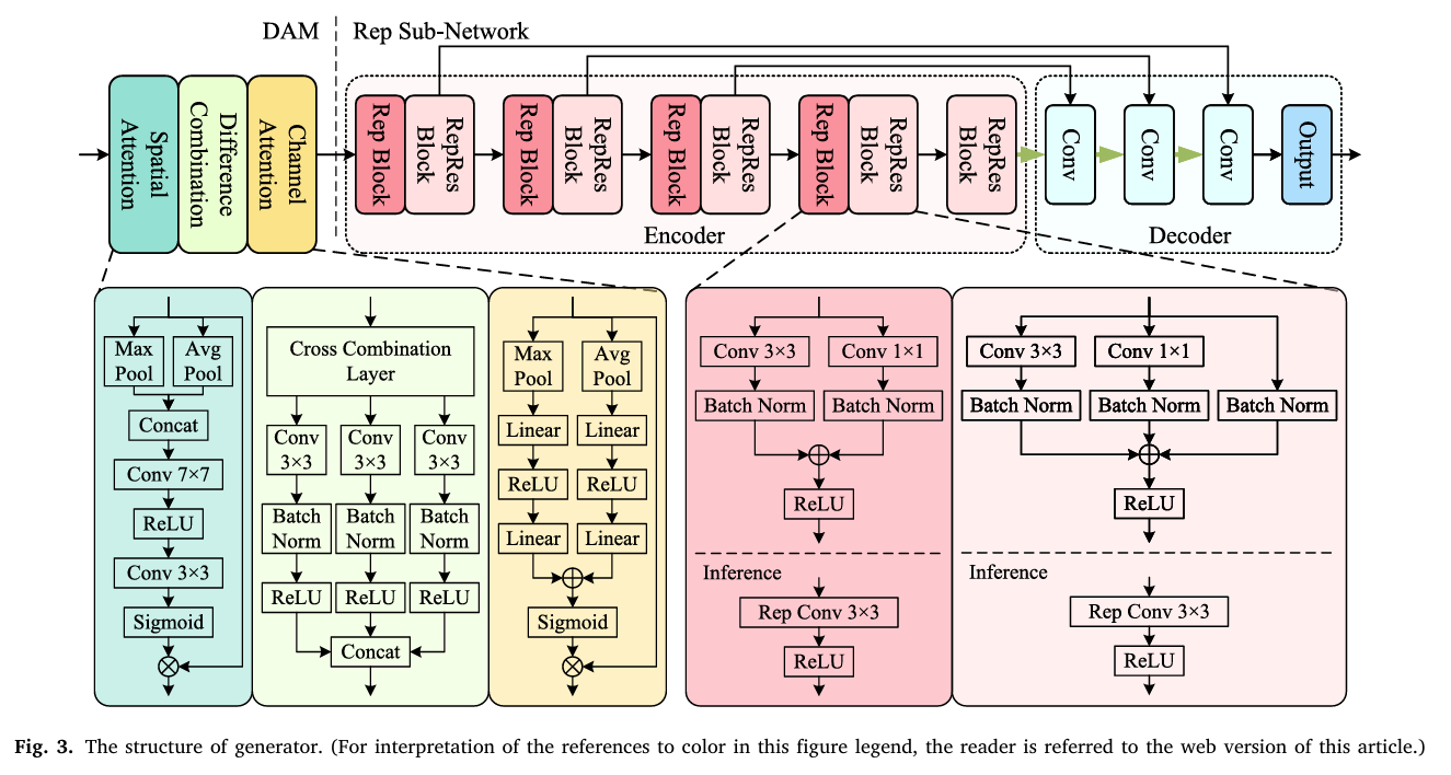
RepVIS-GAN attacks the accuracy problem with the Difference Attention Module (DAM) — a cross-combination strategy that computes all pairwise inter-channel differences, weights them with spatial attention, and routes them through channel attention before any encoding. It attacks the speed problem with structural reparameterization — multi-branch Rep and RepRes blocks during training that collapse to single-branch convolutions at inference, preserving representation capacity while dramatically reducing latency.
The RepVIS-GAN Architecture
The Difference Attention Module — Why Channel Differences Matter
Step 1: Spatial Attention — Weighting What to Look At
Before any cross-channel computation happens, the DAM first asks a simpler question: which spatial regions are most informative? The spatial attention block combines max-pooled and average-pooled versions of the input, processes them through 3×3 and 7×7 convolutions, and produces a spatial weight map \(W_s\). Each channel of the input is independently scaled by this shared spatial attention weight:
This step concentrates subsequent computations on spatially meaningful areas — cloud boundaries, coastlines, convective towers — rather than treating all pixels equally.
Step 2: The Cross Combination Layer — Computing What’s Different
The key insight in DAM is that inter-channel differences encode physically meaningful information that individual channels cannot express alone. The difference between the 3.75 μm and 10.70 μm channels separates fire-detection signatures from background radiation. The 7.10 μm minus 10.70 μm difference captures mid-tropospheric moisture gradients. These physical relationships are explicitly computed by the cross combination layer:
Each of the three pairwise combinations is processed through its own convolution-BN-ReLU block, producing a 3-channel feature tensor per pair, which are concatenated into a 9-channel output \(D\). This is richer than simply computing differences and feeding them directly — each pair’s combined features are learned, not hand-crafted.
Step 3: Channel Attention — Reweighting What Matters
The 9-channel difference feature tensor \(D\) is then passed through a Squeeze-and-Excitation-style channel attention block. Global max-pooling and average-pooling compress each channel to a scalar, which are fed through two-layer MLPs with 9 hidden neurons and combined via sigmoid to produce channel weights \(W_c\). The final DAM output \(O = W_c \otimes D\) is a channel-reweighted version of the difference features — the network has learned which pairwise channel combinations are most informative for predicting visible reflectance.
Structural Reparameterization — The Speed Trick That Doesn’t Cost Accuracy
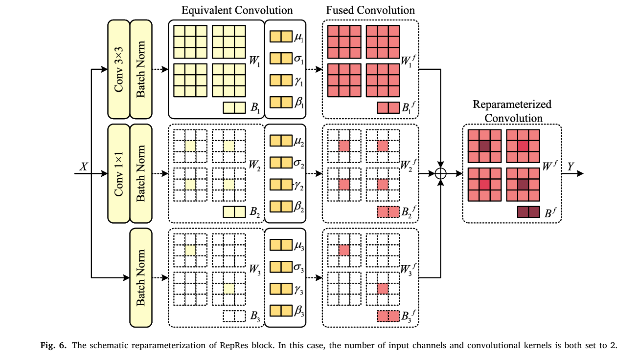
The Rep and RepRes blocks implement a training-inference duality borrowed from RepVGG. During training, multiple parallel branches compute different transformations of the same input and sum their outputs. During inference, those branches are fused into a single equivalent convolution that produces identical results with a fraction of the compute.
For the RepRes block (which has three branches), the fusion works as follows. Each branch produces a convolution-with-BatchNorm operation \(Y_n = X * W_n + B_n\) followed by BN normalization. After training, BN parameters \((\mu_n, \sigma_n, \gamma_n, \beta_n)\) are absorbed into the convolution weights:
The 1×1 convolution branch gets padded with zeros to become an equivalent 3×3 kernel. The identity/residual branch is treated as a 1×1 convolution with an identity weight matrix, then also zero-padded to 3×3. All three fused 3×3 kernels are summed into a single kernel and bias. At inference, the RepRes block is just one Conv3×3 — with no extra memory fetches, branching logic, or BN computations. The same process applies to the two-branch Rep block. This is why reparameterization cuts the nationwide China retrieval from 13.96 minutes to 4.54 minutes: the architectural complexity stays in the gradient graphs during training but disappears at deployment.
“By decoupling the training and inference phases, the technology adopts complex multi-branch architecture during training to enhance feature learning while transforming them into a simpler and computationally efficient single-branch model for inference.” — Si, Li & Han, ISPRS Journal of Photogrammetry and Remote Sensing, 2026
Results: How Much Does Each Piece Contribute?
Comparison Against Baselines on FY-4A Test Set
| Method | MAE ↓ | RMSE ↓ | PSNR ↑ | ERGAS ↓ | CC ↑ | SSIM ↑ |
|---|---|---|---|---|---|---|
| VGG | 21.56 | 28.06 | 19.86 | 11.22 | 0.748 | 0.724 |
| U-Net | 18.78 | 24.99 | 21.10 | 9.68 | 0.799 | 0.757 |
| Pix2pix | 16.56 | 22.85 | 22.15 | 8.63 | 0.861 | 0.823 |
| SE-GAN | 15.94 | 21.88 | 22.52 | 8.23 | 0.894 | 0.839 |
| RepVIS-GAN (ours) | 13.87 | 19.37 | 23.48 | 7.38 | 0.911 | 0.873 |
Ablation Study — Every Component Earns Its Place
| Scheme | Preprocess | Module | Encoder | MAE ↓ | PSNR ↑ | SSIM ↑ |
|---|---|---|---|---|---|---|
| Baseline | BI | None | SC | 17.27 | 20.57 | 0.810 |
| + Rep structure | BI | None | RS | 16.97 | 21.69 | 0.822 |
| + DAM (full model) | BI | DAM | RS | 13.87 | 23.48 | 0.873 |
| No bilinear interpolation | — | DAM | RS | 18.36 | 22.99 | 0.807 |
Computational Efficiency on China Region
| Network | Params (M) | Avg Time / Image (s) | China Total (min) |
|---|---|---|---|
| VIS-GAN (no reparam.) | 2.90 | 11.17 | 13.96 |
| SE-GAN | 1.94 | 3.55 | 4.99 |
| RepVGG (reparameterized) | 2.69 | 3.60 | 4.90 |
| RepVIS-GAN (reparameterized) | 2.70 | 3.46 | 4.54 |
Complete End-to-End RepVIS-GAN Implementation (PyTorch)
The implementation covers all components from the paper in 12 sections: the Spatial Attention Block, the Cross Combination (Difference) Layer, the Channel Attention Block, the full Difference Attention Module (DAM), the Rep and RepRes reparameterized convolutional blocks with BN fusion, the Rep Sub-Network encoder and decoder, the full Generator, the PatchGAN-style Discriminator with Rep/RepRes blocks, the mixed loss function (adversarial + MAE + SSIM), evaluation metrics, the complete RepVIS-GAN training loop, and a smoke test.
# ==============================================================================
# RepVIS-GAN: A Reparameterized GAN-Based Network for Visible Image
# Retrieval from Geostationary Satellite Infrared Observations
# Paper: ISPRS Journal of Photogrammetry and Remote Sensing 236 (2026) 162-174
# Authors: Jianwei Si, Chuanxin Li, Lei Han
# Affiliation: Ocean University of China / CMA Tornado Key Lab
# DOI: https://doi.org/10.1016/j.isprsjprs.2026.03.025
# ==============================================================================
# Sections:
# 1. Imports & Configuration
# 2. Spatial Attention Block (Section 3.1.1, Eq. 1)
# 3. Cross Combination (Difference) Layer (Eq. 2-5)
# 4. Channel Attention Block (Eq. 6-7)
# 5. Full Difference Attention Module — DAM
# 6. Rep Block (2-branch reparameterized convolution)
# 7. RepRes Block (3-branch reparameterized residual convolution, Eq. 17-23)
# 8. Rep Sub-Network: Encoder + Decoder
# 9. Full Generator (DAM + Rep Sub-Network)
# 10. PatchGAN Discriminator with Rep/RepRes blocks
# 11. Loss Functions + Evaluation Metrics (Eq. 8-16, 24-30)
# 12. Training Loop + Smoke Test
# ==============================================================================
from __future__ import annotations
import math, warnings
from typing import Dict, List, Optional, Tuple
import torch
import torch.nn as nn
import torch.nn.functional as F
from torch import Tensor
warnings.filterwarnings("ignore")
# ─── SECTION 1: Configuration ─────────────────────────────────────────────────
class RepVISConfig:
"""
RepVIS-GAN hyperparameters matching paper's FY-4A training setup.
Input: 3 IR channels (CH08=3.75μm, CH10=7.10μm, CH12=10.70μm)
bilinearly interpolated to 1km resolution: (B, 3, 600, 600)
Output: 1-channel VIS reflectance at 0.65μm: (B, 1, 600, 600)
"""
in_channels: int = 3 # CH08, CH10, CH12 infrared inputs
out_channels: int = 1 # CH02 (0.65μm) visible output
img_size: int = 600 # 600×600 pixel tiles
dam_hidden: int = 9 # neurons in channel attention FC layers
# Encoder channel progression (Rep groups)
enc_channels: List = [32, 64, 128, 256] # output channels per encoder group
enc_strides: List = [1, 2, 2, 2] # downsampling at groups 2-4
# Decoder
dec_channels: List = [128, 128, 64, 64, 32, 32]
dropout_p: float = 0.1
# Loss weights (Eq. 8): λ1=1 (gan), λ2=5 (mae), λ3=5 (ssim)
lambda_gan: float = 1.0
lambda_mae: float = 5.0
lambda_ssim: float = 5.0
lambda_d_real: float = 0.5 # λ4 (Eq. 16)
lambda_d_fake: float = 0.5 # λ5
# Training
lr: float = 1e-4
batch_size: int = 8
n_epochs: int = 100
ssim_C1: float = (0.01 * 255)**2 # = 6.5025 (Eq. 12)
ssim_C2: float = (0.03 * 255)**2 # = 58.5225
ergas_scale: float = 0.25 # scale factor r in ERGAS (Eq. 27)
def __init__(self, **kwargs):
for k, v in kwargs.items(): setattr(self, k, v)
# ─── SECTION 2: Spatial Attention Block ───────────────────────────────────────
class SpatialAttentionBlock(nn.Module):
"""
Spatial Attention Block in DAM (Section 3.1.1, Eq. 1).
Produces a spatial weight map W_s that highlights the most
informative spatial regions across all input IR channels.
Uses max-pooling + average-pooling to extract channel-wise statistics,
then 3×3 and 7×7 convolutions to compute the spatial map.
s_m = W_s ⊗ F_m (each channel weighted by same spatial map)
The 7×7 conv captures broader structural context (cloud systems),
while 3×3 focuses on fine-grained local texture (cloud edges).
Both are applied to the concatenated pooling outputs.
"""
def __init__(self):
super().__init__()
# After channel max+avg pool: 2-channel spatial descriptor
self.conv3 = nn.Conv2d(2, 1, kernel_size=3, padding=1)
self.conv7 = nn.Conv2d(2, 1, kernel_size=7, padding=3)
self.relu = nn.ReLU(inplace=True)
self.sigmoid = nn.Sigmoid()
def forward(self, x: Tensor) -> Tuple[Tensor, List[Tensor]]:
"""
x: (B, C, H, W) — multi-channel IR input F
Returns: W_s (B,1,H,W), spatial-weighted channels [s1, s2, ..., sC]
"""
# Channel max and avg pooling → compress C channels to 2
max_pool = x.max(dim=1, keepdim=True).values # (B,1,H,W)
avg_pool = x.mean(dim=1, keepdim=True) # (B,1,H,W)
pool_cat = torch.cat([max_pool, avg_pool], dim=1) # (B,2,H,W)
# Multi-scale spatial attention
s3 = self.relu(self.conv3(pool_cat))
s7 = self.relu(self.conv7(pool_cat))
W_s = self.sigmoid(s3 + s7) # (B,1,H,W)
# Per-channel spatial weighting: s_m = W_s ⊗ F_m (Eq. 1)
channels = [W_s * x[:, m:m+1, :, :] for m in range(x.shape[1])]
return W_s, channels # W_s: (B,1,H,W), channels: list of (B,1,H,W)
# ─── SECTION 3: Cross Combination (Difference) Layer ──────────────────────────
class CrossCombinationLayer(nn.Module):
"""
Difference Combination Block (Section 3.1.1, Eq. 2-5).
Computes ALL pairwise absolute differences between spatially-attended
channels and concatenates them with the original channels.
This makes inter-channel physical relationships explicit:
- |s_CH08 - s_CH10|: thermal vs moisture contrast (cloud type indicator)
- |s_CH08 - s_CH12|: surface/cloud temperature differential
- |s_CH10 - s_CH12|: moisture-thermal interaction
Each triplet (s_p, s_q, d_pq) is processed by its own Conv-BN-ReLU
to learn task-specific feature combinations per channel pair.
"""
def __init__(self, n_channels: int = 3, out_ch_per_pair: int = 3):
super().__init__()
self.n_channels = n_channels
# Number of pairs = C*(C-1)//2 for C input channels
pairs = [(p, q) for p in range(n_channels) for q in range(p+1, n_channels)]
self.pairs = pairs
n_pairs = len(pairs)
# One Conv3×3-BN-ReLU per pair (input: 3 channels = s_p + s_q + d_pq)
self.pair_convs = nn.ModuleList([
nn.Sequential(
nn.Conv2d(3, out_ch_per_pair, kernel_size=3, padding=1),
nn.BatchNorm2d(out_ch_per_pair),
nn.ReLU(inplace=True),
)
for _ in range(n_pairs)
])
self.out_channels = n_pairs * out_ch_per_pair
def forward(self, channels: List[Tensor]) -> Tensor:
"""
channels: list of C tensors each (B,1,H,W) — spatially weighted IR channels
Returns: D (B, n_pairs*out_ch, H, W) — difference-enriched features
"""
D_parts = []
for idx, (p, q) in enumerate(self.pairs):
sp, sq = channels[p], channels[q]
d_pq = torch.abs(sp - sq) # |s_p - s_q| (Eq. 2)
dc_pq = torch.cat([sp, sq, d_pq], dim=1) # concat (Eq. 3)
D_k = self.pair_convs[idx](dc_pq) # Conv-BN-ReLU (Eq. 4)
D_parts.append(D_k)
D = torch.cat(D_parts, dim=1) # concat (Eq. 5)
return D # (B, n_pairs*out_ch, H, W)
# ─── SECTION 4: Channel Attention Block ───────────────────────────────────────
class ChannelAttentionBlock(nn.Module):
"""
SE-style channel attention block in DAM (Section 3.1.1, Eq. 6-7).
W_c = η(L2(σ(L1(MaxPool(D)))) + L4(σ(L3(AvgPool(D)))))
O = W_c ⊗ D
After computing all pairwise differences, this block reweights
the 9 feature channels to emphasize those most relevant for
visible reflectance prediction. With 9 hidden neurons in all
linear layers, it learns a compact channel importance vector.
"""
def __init__(self, in_ch: int, hidden: int = 9):
super().__init__()
# Max-pool path: MaxPool → L1(σ) → L2
self.max_path = nn.Sequential(
nn.AdaptiveMaxPool2d(1),
nn.Flatten(),
nn.Linear(in_ch, hidden),
nn.ReLU(),
nn.Linear(hidden, in_ch),
)
# Avg-pool path: AvgPool → L3(σ) → L4
self.avg_path = nn.Sequential(
nn.AdaptiveAvgPool2d(1),
nn.Flatten(),
nn.Linear(in_ch, hidden),
nn.ReLU(),
nn.Linear(hidden, in_ch),
)
self.sigmoid = nn.Sigmoid()
def forward(self, D: Tensor) -> Tensor:
"""
D: (B, C, H, W) — difference features from CrossCombinationLayer
Returns: O = W_c ⊗ D (B, C, H, W) channel-reweighted features
"""
B, C, H, W = D.shape
W_c_raw = self.max_path(D) + self.avg_path(D) # (B, C)
W_c = self.sigmoid(W_c_raw).unsqueeze(-1).unsqueeze(-1) # (B,C,1,1)
O = W_c * D # (B, C, H, W)
return O
# ─── SECTION 5: Full Difference Attention Module (DAM) ────────────────────────
class DifferenceAttentionModule(nn.Module):
"""
Difference Attention Module (DAM) — the core feature extractor of RepVIS-GAN.
Design motivation: conventional spatial or channel attention handles each
IR channel independently, missing inter-channel physical relationships.
DAM explicitly models ALL pairwise differences because they encode:
- Cloud phase and height (BT differences between windows and water vapor)
- Surface emissivity patterns (mid-wave vs long-wave window)
- Atmospheric moisture gradients (water vapor channel differences)
Three-stage pipeline (Section 3.1.1):
1. Spatial attention: weight pixels by their spatial informativeness
2. Difference combination: compute and learn from all channel pair diffs
3. Channel attention: reweight the 9 resulting difference feature channels
Ablation study confirms DAM beats both SE and CBAM attention modules:
No attention → MAE=16.97 (Scheme 9)
SE module → MAE=14.88 (Scheme 10)
CBAM module → MAE=14.49 (Scheme 11)
DAM (ours) → MAE=13.87 (Scheme 12, best)
"""
def __init__(self, in_channels: int = 3, out_ch_per_pair: int = 3, ca_hidden: int = 9):
super().__init__()
self.spatial_attn = SpatialAttentionBlock()
self.diff_combo = CrossCombinationLayer(in_channels, out_ch_per_pair)
diff_out_ch = self.diff_combo.out_channels # 9 for 3 channels, 3 ch/pair
self.channel_attn = ChannelAttentionBlock(diff_out_ch, ca_hidden)
self.out_channels = diff_out_ch
def forward(self, x: Tensor) -> Tensor:
"""
x: (B, 3, H, W) — concatenated IR channel inputs (CH08, CH10, CH12)
Returns: O (B, 9, H, W) — spatial+difference+channel attention features
"""
# Step 1: Spatial attention → per-channel weighted outputs
_, channels = self.spatial_attn(x) # list of 3×(B,1,H,W)
# Step 2: Difference combination → 9-channel feature map D
D = self.diff_combo(channels) # (B,9,H,W)
# Step 3: Channel attention → reweighted output O
O = self.channel_attn(D) # (B,9,H,W)
return O
# ─── SECTION 6: Rep Block ─────────────────────────────────────────────────────
class RepBlock(nn.Module):
"""
Reparameterized Convolutional Block (2-branch, Section 3.1.2 / 3.4).
TRAINING: Two parallel branches (3×3 conv + 1×1 conv), each with BN.
Y_1 = BN_1(X * W_1_3x3) [3×3 convolution branch]
Y_2 = BN_2(X * W_2_1x1) [1×1 convolution branch]
Output = ReLU(Y_1 + Y_2)
INFERENCE: Branches fused into single equivalent 3×3 convolution:
W_f = W_f_1 + W_f_2 (pad 1×1 kernel with zeros to 3×3 before summing)
B_f = B_f_1 + B_f_2
Y_r = ReLU(X * W_f + B_f)
Fusion: absorb BN into conv (Eq. 20-21):
W_f_n = (γ_n * W_n) / sqrt(σ²_n + ε)
B_f_n = γ_n*(B_n - μ_n)/sqrt(σ²_n + ε) + β_n
Benefits:
- Training: multi-branch diversity → richer gradient signal
- Inference: single-branch → no branching overhead, faster memory access
"""
def __init__(self, in_ch: int, out_ch: int, stride: int = 1):
super().__init__()
self.in_ch = in_ch; self.out_ch = out_ch; self.stride = stride
self.training_mode = True
# Branch 1: 3×3 conv + BN
self.branch_3x3 = nn.Conv2d(in_ch, out_ch, 3, stride=stride, padding=1, bias=False)
self.bn_3x3 = nn.BatchNorm2d(out_ch)
# Branch 2: 1×1 conv + BN
self.branch_1x1 = nn.Conv2d(in_ch, out_ch, 1, stride=stride, padding=0, bias=False)
self.bn_1x1 = nn.BatchNorm2d(out_ch)
self.relu = nn.ReLU(inplace=True)
# Fused inference convolution (filled in by reparameterize())
self.fused_conv: Optional[nn.Conv2d] = None
def forward(self, x: Tensor) -> Tensor:
if self.fused_conv is not None:
# Inference mode: single fused convolution
return self.relu(self.fused_conv(x))
# Training mode: multi-branch sum
y1 = self.bn_3x3(self.branch_3x3(x))
y2 = self.bn_1x1(self.branch_1x1(x))
return self.relu(y1 + y2)
@staticmethod
def _fuse_bn(conv: nn.Conv2d, bn: nn.BatchNorm2d) -> Tuple[Tensor, Tensor]:
"""Absorb BN parameters into conv kernel and bias (Eq. 20-21)."""
W = conv.weight # (out, in, kH, kW)
gamma = bn.weight # γ (out,)
beta = bn.bias # β (out,)
mean = bn.running_mean # μ (out,)
var = bn.running_var # σ² (out,)
eps = bn.eps
std = (var + eps).sqrt()
W_f = (gamma / std).view(-1, 1, 1, 1) * W
B_f = beta - gamma * mean / std
return W_f, B_f
def reparameterize(self):
"""
Fuse all branches into one single 3×3 convolution for inference.
1×1 kernel padded to 3×3, then all fused kernels are summed.
Call this ONCE after training is complete, before deployment.
"""
W3, B3 = self._fuse_bn(self.branch_3x3, self.bn_3x3)
# Pad 1×1 kernel to 3×3 with zeros (Eq. 19 discussion)
W1, B1 = self._fuse_bn(self.branch_1x1, self.bn_1x1)
W1_padded = F.pad(W1, [1, 1, 1, 1]) # (out,in,3,3) with zeros around center
# Fuse: sum all branches (Eq. 23)
W_f = W3 + W1_padded
B_f = B3 + B1
self.fused_conv = nn.Conv2d(
self.in_ch, self.out_ch, 3, stride=self.stride, padding=1
)
self.fused_conv.weight.data.copy_(W_f)
self.fused_conv.bias.data.copy_(B_f)
# Free training branch memory
del self.branch_3x3, self.bn_3x3, self.branch_1x1, self.bn_1x1
# ─── SECTION 7: RepRes Block ──────────────────────────────────────────────────
class RepResBlock(nn.Module):
"""
Reparameterized Residual Convolutional Block (3-branch, Eq. 17-22).
TRAINING: Three parallel branches:
Branch 1: Conv3×3 + BN (main feature extraction)
Branch 2: Conv1×1 + BN (cross-channel mixing, zero pad to 3×3 for fusion)
Branch 3: Identity + BN (residual, treated as 1×1 with identity kernel)
All three branches share the same input, and their outputs are summed:
Y = ReLU(Σ_n (X * W_n + B_n)) → after BN absorption: Y = ReLU(X * W_f + B_f)
INFERENCE: Single fused 3×3 convolution (no branching).
The residual branch requires in_ch == out_ch. When stride=1 and channels
match, RepRes provides an implicit residual connection analogous to
standard ResNet blocks but without explicit skip-connection memory.
Ablation validates superiority over plain SC and Res blocks:
SC (standard): MAE=15.98 (Scheme 6)
Res blocks: MAE=15.20 (Scheme 7)
RS (Rep+RepRes): MAE=13.87 (Scheme 8, best)
"""
def __init__(self, in_ch: int, out_ch: int, stride: int = 1):
super().__init__()
self.in_ch = in_ch; self.out_ch = out_ch; self.stride = stride
self.has_residual = (in_ch == out_ch) and (stride == 1)
# Branch 1: 3×3 conv + BN
self.branch_3x3 = nn.Conv2d(in_ch, out_ch, 3, stride=stride, padding=1, bias=False)
self.bn_3x3 = nn.BatchNorm2d(out_ch)
# Branch 2: 1×1 conv + BN
self.branch_1x1 = nn.Conv2d(in_ch, out_ch, 1, stride=stride, padding=0, bias=False)
self.bn_1x1 = nn.BatchNorm2d(out_ch)
# Branch 3: Identity (residual) + BN — only when in_ch==out_ch, stride==1
if self.has_residual:
self.bn_identity = nn.BatchNorm2d(in_ch)
self.relu = nn.ReLU(inplace=True)
self.fused_conv: Optional[nn.Conv2d] = None
def forward(self, x: Tensor) -> Tensor:
if self.fused_conv is not None:
return self.relu(self.fused_conv(x))
y1 = self.bn_3x3(self.branch_3x3(x))
y2 = self.bn_1x1(self.branch_1x1(x))
y_sum = y1 + y2
if self.has_residual:
y_sum = y_sum + self.bn_identity(x) # residual branch (Eq. 17)
return self.relu(y_sum)
@staticmethod
def _fuse_bn(W: Tensor, B: Optional[Tensor], bn: nn.BatchNorm2d) -> Tuple[Tensor, Tensor]:
gamma = bn.weight
beta = bn.bias
mean = bn.running_mean
var = bn.running_var
std = (var + bn.eps).sqrt()
W_f = (gamma / std).view(-1, 1, 1, 1) * W
B_out = (B if B is not None else torch.zeros(W.shape[0], device=W.device))
B_f = beta - gamma * mean / std + gamma * B_out / std
return W_f, B_f
def reparameterize(self):
"""Fuse all 3 branches into one 3×3 conv (Eq. 22)."""
W3, B3 = RepBlock._fuse_bn(self.branch_3x3, self.bn_3x3)
W1, B1 = RepBlock._fuse_bn(self.branch_1x1, self.bn_1x1)
W1_pad = F.pad(W1, [1, 1, 1, 1]) # 1×1 → 3×3 via zero padding
W_f = W3 + W1_pad
B_f = B3 + B1
if self.has_residual:
# Identity branch: weight = identity matrix per channel (unit matrix)
# Treated as 1×1 conv with weight I, then padded to 3×3
C = self.in_ch
W_id = torch.eye(C, device=W3.device).view(C, C, 1, 1)
W_id_pad = F.pad(W_id, [1, 1, 1, 1])
bn_id = self.bn_identity
gamma = bn_id.weight; beta = bn_id.bias
mean = bn_id.running_mean; var = bn_id.running_var
std = (var + bn_id.eps).sqrt()
W_id_f = (gamma / std).view(-1, 1, 1, 1) * W_id_pad
B_id_f = beta - gamma * mean / std
W_f = W_f + W_id_f
B_f = B_f + B_id_f
self.fused_conv = nn.Conv2d(self.in_ch, self.out_ch, 3, stride=self.stride, padding=1)
self.fused_conv.weight.data.copy_(W_f)
self.fused_conv.bias.data.copy_(B_f)
del self.branch_3x3, self.bn_3x3, self.branch_1x1, self.bn_1x1
if self.has_residual:
del self.bn_identity
def reparameterize_all(module: nn.Module):
"""
Recursively reparameterize all Rep and RepRes blocks in a network.
Call once after training: model.eval(); reparameterize_all(model)
This collapses multi-branch training structure into single-branch inference.
"""
for child in module.children():
if isinstance(child, (RepBlock, RepResBlock)):
child.reparameterize()
else:
reparameterize_all(child)
# ─── SECTION 8: Rep Sub-Network Encoder + Decoder ─────────────────────────────
class RepEncoder(nn.Module):
"""
Rep Sub-Network Encoder (Section 3.1.2).
4 groups of alternating Rep + RepRes blocks for progressive downsampling.
Input: DAM output O (B, 9, H, W)
Output: 4 feature maps at progressively lower resolution (for skip connections)
Group 1 (expand): Rep[9→32,s=1] + RepRes[32,s=1]
Group 2 (downsample): Rep[32→64,s=2] + RepRes[64,s=1]
Group 3 (downsample): Rep[64→128,s=2]+ RepRes[128,s=1]
Group 4 (downsample): Rep[128→256,s=2]+RepRes[256,s=1]
Extra: RepRes[256,s=1] (deepest representation)
"""
def __init__(self, in_ch: int = 9):
super().__init__()
# (in_ch, out_ch, stride) per group
cfg = [(in_ch, 32, 1), (32, 64, 2), (64, 128, 2), (128, 256, 2)]
self.groups = nn.ModuleList()
for ic, oc, st in cfg:
self.groups.append(nn.Sequential(
RepBlock(ic, oc, stride=st),
RepResBlock(oc, oc, stride=1),
))
# Extra RepRes at deepest level
self.extra_rep = RepResBlock(256, 256, stride=1)
def forward(self, x: Tensor) -> Tuple[Tensor, List[Tensor]]:
"""
Returns: (bottleneck, skips)
bottleneck: (B, 256, H/8, W/8) — deepest features
skips: list of 4 tensors for decoder skip connections
"""
skips = []
h = x
for group in self.groups:
h = group(h)
skips.append(h)
h = self.extra_rep(h)
return h, skips # (bottleneck, [32,64,128,256] feature maps)
class ConvBlock(nn.Module):
"""Decoder ConvBlock: two 3×3 convs + Dropout + BN + ReLU (×2)."""
def __init__(self, in_ch: int, out_ch: int, dropout_p: float = 0.1):
super().__init__()
self.block = nn.Sequential(
nn.Conv2d(in_ch, out_ch, 3, padding=1), nn.Dropout2d(dropout_p),
nn.BatchNorm2d(out_ch), nn.ReLU(inplace=True),
nn.Conv2d(out_ch, out_ch, 3, padding=1), nn.Dropout2d(dropout_p),
nn.BatchNorm2d(out_ch), nn.ReLU(inplace=True),
)
def forward(self, x: Tensor) -> Tensor: return self.block(x)
class RepDecoder(nn.Module):
"""
Rep Sub-Network Decoder (Section 3.1.2).
Three transposed-conv upsampling stages with skip connections from encoder.
Each stage: TransposeConv(2×2,s=2) + concat(skip) → ConvBlock.
Final output block: Conv3×3(16) → BN → ReLU → Conv3×3(1) → retrieved VIS.
"""
def __init__(self, out_channels: int = 1, dropout_p: float = 0.1):
super().__init__()
# Three upsampling stages; skip channel counts: [256,128,64,32]
# After concat: 256+256=512, 128+128=256, 64+64=128 (simplified)
self.up1 = nn.ConvTranspose2d(256, 128, 2, stride=2)
self.cb1 = ConvBlock(128 + 128, 128, dropout_p)
self.up2 = nn.ConvTranspose2d(128, 64, 2, stride=2)
self.cb2 = ConvBlock(64 + 64, 64, dropout_p)
self.up3 = nn.ConvTranspose2d(64, 32, 2, stride=2)
self.cb3 = ConvBlock(32 + 32, 32, dropout_p)
# Output block: Conv3×3(16) → BN → ReLU → Conv3×3(1)
self.out_block = nn.Sequential(
nn.Conv2d(32, 16, 3, padding=1),
nn.BatchNorm2d(16),
nn.ReLU(inplace=True),
nn.Conv2d(16, out_channels, 3, padding=1),
)
def forward(self, bottleneck: Tensor, skips: List[Tensor]) -> Tensor:
"""
bottleneck: (B,256,H/8,W/8)
skips: [enc_32, enc_64, enc_128, enc_256] from encoder groups
Returns: ŷ (B,1,H,W) — retrieved visible reflectance
"""
x = self.up1(bottleneck)
if x.shape[-2:] != skips[2].shape[-2:]:
x = F.interpolate(x, size=skips[2].shape[-2:], mode='bilinear', align_corners=False)
x = self.cb1(torch.cat([x, skips[2]], dim=1)) # skip from group 3 (128ch)
x = self.up2(x)
if x.shape[-2:] != skips[1].shape[-2:]:
x = F.interpolate(x, size=skips[1].shape[-2:], mode='bilinear', align_corners=False)
x = self.cb2(torch.cat([x, skips[1]], dim=1)) # skip from group 2 (64ch)
x = self.up3(x)
if x.shape[-2:] != skips[0].shape[-2:]:
x = F.interpolate(x, size=skips[0].shape[-2:], mode='bilinear', align_corners=False)
x = self.cb3(torch.cat([x, skips[0]], dim=1)) # skip from group 1 (32ch)
return self.out_block(x) # ŷ: (B,1,H,W)
# ─── SECTION 9: Full Generator ────────────────────────────────────────────────
class RepVISGenerator(nn.Module):
"""
RepVIS-GAN Generator (Section 3.1, Fig. 3).
Full pipeline: IR input → DAM → Rep Encoder → Rep Decoder → VIS output
Training: multi-branch Rep/RepRes blocks for representation diversity
Inference: reparameterized single-branch — 11.17s → 3.46s per tile
"""
def __init__(self, cfg: RepVISConfig):
super().__init__()
self.dam = DifferenceAttentionModule(cfg.in_channels)
self.encoder = RepEncoder(in_ch=self.dam.out_channels)
self.decoder = RepDecoder(cfg.out_channels, cfg.dropout_p)
def forward(self, ir: Tensor) -> Tensor:
"""
ir: (B, 3, H, W) — stacked IR channels (CH08, CH10, CH12)
Returns ŷ: (B, 1, H, W) — retrieved visible reflectance [0-255 range]
"""
O = self.dam(ir) # (B,9,H,W)
bottleneck, skips = self.encoder(O) # hierarchical features
y_hat = self.decoder(bottleneck, skips) # (B,1,H,W)
return y_hat
# ─── SECTION 10: PatchGAN Discriminator ───────────────────────────────────────
class RepVISDiscriminator(nn.Module):
"""
PatchGAN Discriminator with Rep and RepRes blocks (Section 3.2, Fig. 5).
PatchGAN principle (Isola et al., 2017): classify whether overlapping
image patches are real or fake, not the entire image at once. This is
more effective at capturing local fine-grained features (cloud texture,
coastline sharpness) rather than global scene plausibility.
Architecture: Rep[64,s=2] → RepRes[64] → Rep[128,s=2] → RepRes[128]
→ Rep[256,s=2] → Conv[256] → Conv[64] → Conv[1,s=2]
"""
def __init__(self, in_channels: int = 1):
super().__init__()
self.features = nn.Sequential(
RepBlock(in_channels, 64, stride=2),
RepResBlock(64, 64, stride=1),
RepBlock(64, 128, stride=2),
RepResBlock(128, 128, stride=1),
RepBlock(128, 256, stride=2),
)
self.classifier = nn.Sequential(
nn.Conv2d(256, 256, 3, stride=2, padding=1),
nn.LeakyReLU(0.2, inplace=True),
nn.Conv2d(256, 64, 3, stride=1, padding=1),
nn.LeakyReLU(0.2, inplace=True),
nn.Conv2d(64, 1, 3, stride=2, padding=1),
nn.Sigmoid(),
)
def forward(self, x: Tensor) -> Tensor:
"""
x: (B, 1, H, W) — real or generated VIS image
Returns patch-level real/fake scores (B, 1, H', W')
"""
feat = self.features(x)
return self.classifier(feat)
# ─── SECTION 11: Loss Functions + Evaluation Metrics ─────────────────────────
def ssim_loss(y: Tensor, y_hat: Tensor, C1: float = 6.5025, C2: float = 58.5225) -> Tensor:
"""
SSIM Loss: L_ssim = 1 - SSIM(y, ŷ) (Eq. 11-15).
SSIM evaluates structural similarity through luminance (mean),
contrast (variance), and structure (covariance) terms.
Combined with MAE, it preserves perceptual quality beyond pixel accuracy.
"""
mu_y = y.mean(dim=[-2,-1], keepdim=True)
mu_yhat = y_hat.mean(dim=[-2,-1], keepdim=True)
sigma_y = y.var(dim=[-2,-1], keepdim=True, unbiased=False)
sigma_yhat = y_hat.var(dim=[-2,-1], keepdim=True, unbiased=False)
sigma_cross = ((y - mu_y) * (y_hat - mu_yhat)).mean(dim=[-2,-1], keepdim=True)
ssim_val = ((2*mu_y*mu_yhat + C1) * (2*sigma_cross + C2)) / \
((mu_y**2 + mu_yhat**2 + C1) * (sigma_y + sigma_yhat + C2))
return (1.0 - ssim_val).mean()
class RepVISLoss(nn.Module):
"""
Mixed generator loss and discriminator loss (Eq. 8-16).
Generator loss:
L_G = λ1·L_gan + λ2·L_mae + λ3·L_ssim
λ1=1, λ2=5, λ3=5 (emphasize pixel accuracy and structural similarity)
Discriminator loss:
L_D = -λ4·log(D(y)) - λ5·log(1 - D(ŷ))
λ4 = λ5 = 0.5 (symmetric real/fake weighting)
The SSIM loss is weighted equally with MAE (both λ=5) because:
- MAE alone produces blurry outputs by averaging solutions
- SSIM enforces structural consistency (luminance, contrast, structure)
- Together they balance pixel accuracy with perceptual quality
"""
def __init__(self, cfg: RepVISConfig):
super().__init__()
self.cfg = cfg
def generator_loss(self, y: Tensor, y_hat: Tensor, d_fake: Tensor) -> Dict[str, Tensor]:
"""
y: (B,1,H,W) ground truth VIS
y_hat: (B,1,H,W) generated VIS
d_fake: (B,1,H',W') discriminator output on generated image
"""
cfg = self.cfg
# L_gan = -log(D(ŷ)): generator fools discriminator (Eq. 9)
eps = 1e-7
l_gan = -torch.log(d_fake + eps).mean()
# L_mae = ||y - ŷ||_1 (Eq. 10)
l_mae = F.l1_loss(y_hat, y)
# L_ssim = 1 - SSIM(y, ŷ) (Eq. 11)
l_ssim = ssim_loss(y, y_hat, cfg.ssim_C1, cfg.ssim_C2)
# Combined (Eq. 8)
l_g = cfg.lambda_gan * l_gan + cfg.lambda_mae * l_mae + cfg.lambda_ssim * l_ssim
return {'total': l_g, 'gan': l_gan, 'mae': l_mae, 'ssim': l_ssim}
def discriminator_loss(self, d_real: Tensor, d_fake: Tensor) -> Tensor:
"""L_D = -λ4·log(D(y)) - λ5·log(1-D(ŷ)) (Eq. 16)"""
eps = 1e-7
l_real = -self.cfg.lambda_d_real * torch.log(d_real + eps).mean()
l_fake = -self.cfg.lambda_d_fake * torch.log(1 - d_fake + eps).mean()
return l_real + l_fake
def compute_metrics(y: Tensor, y_hat: Tensor, scale_factor: float = 0.25) -> Dict[str, float]:
"""
Compute all evaluation metrics from the paper (Eq. 24-30).
All metrics operate on pixel values in [0,255] range.
MAE: Mean Absolute Error (↓ better)
RMSE: Root Mean Squared Error (↓ better)
PSNR: Peak Signal-to-Noise Ratio (↑ better)
ERGAS: Global relative error index (↓ better)
CC: Pearson Correlation Coefficient (↑ better)
SSIM: Structural Similarity Index (↑ better)
QI: Universal Quality Index (↑ better)
"""
y_np = y.detach().float()
h_np = y_hat.detach().float()
B = y_np.shape[0]
eps = 1e-8
# Flatten spatial dims for statistics
y_flat = y_np.reshape(B, -1)
h_flat = h_np.reshape(B, -1)
mae = (y_flat - h_flat).abs().mean().item()
mse = ((y_flat - h_flat)**2).mean().item()
rmse = math.sqrt(mse)
psnr = 10 * math.log10(255**2 / (mse + eps))
mu_y = y_flat.mean(-1, keepdim=True) # (B,1)
ergas_vals = 100 * scale_factor * (mse**0.5) / (mu_y.squeeze(-1).mean().item() + eps)
ergas = ergas_vals
# CC: Pearson correlation (Eq. 28)
mu_h = h_flat.mean(-1, keepdim=True)
dy = y_flat - mu_y; dh = h_flat - mu_h
cov = (dy * dh).mean(-1)
std_y = dy.std(-1); std_h = dh.std(-1)
cc = (cov / (std_y * std_h + eps)).mean().item()
# SSIM (scalar version)
ssim_val = 1.0 - ssim_loss(y_np, h_np).item()
# QI: Universal Quality Index (Eq. 29)
mu_y_s = mu_y.squeeze(-1); mu_h_s = mu_h.squeeze(-1)
var_y = dy.var(-1, unbiased=False); var_h = dh.var(-1, unbiased=False)
qi = (4 * cov * mu_y_s * mu_h_s /
((mu_y_s**2 + mu_h_s**2 + eps) * (var_y + var_h + eps))).mean().item()
return {'MAE': mae, 'RMSE': rmse, 'PSNR': psnr,
'ERGAS': ergas, 'CC': cc, 'SSIM': ssim_val, 'QI': qi}
# ─── SECTION 12: Training Loop + Smoke Test ───────────────────────────────────
class RepVISGAN(nn.Module):
"""
Complete RepVIS-GAN wrapper combining Generator and Discriminator.
Training: multi-branch Rep/RepRes blocks, mixed G+D loss
Inference: call reparameterize_all(model) then model.generate(ir)
Paper setup:
- Dataset: FY-4A AGRI CH08/CH10/CH12 → CH02
- Train: May–Jul 2019 (5344 samples), Test: Aug 2019 (1591 samples)
- Generalization: May–Aug 2023 (1593 samples)
- Input size: 600×600 @ 1km after bilinear interpolation of 4km IR
- Framework: TensorFlow (paper); this is PyTorch educational equivalent
- Hardware: NVIDIA GPU (paper uses unspecified GPU for experiments)
"""
def __init__(self, cfg: Optional[RepVISConfig] = None):
super().__init__()
cfg = cfg or RepVISConfig()
self.cfg = cfg
self.generator = RepVISGenerator(cfg)
self.discriminator = RepVISDiscriminator(cfg.out_channels)
self.loss_fn = RepVISLoss(cfg)
def generate(self, ir: Tensor) -> Tensor:
"""Inference: IR → VIS. Call reparameterize_all(self) first."""
return self.generator(ir)
def train_step_g(
self,
ir: Tensor, vis_real: Tensor,
opt_g: torch.optim.Optimizer,
) -> Dict[str, float]:
"""Generator training step."""
self.generator.train()
opt_g.zero_grad()
vis_fake = self.generator(ir)
d_fake = self.discriminator(vis_fake)
losses = self.loss_fn.generator_loss(vis_real, vis_fake, d_fake)
losses['total'].backward()
torch.nn.utils.clip_grad_norm_(self.generator.parameters(), 1.0)
opt_g.step()
return {k: v.item() if isinstance(v, Tensor) else v for k, v in losses.items()}
def train_step_d(
self,
ir: Tensor, vis_real: Tensor,
opt_d: torch.optim.Optimizer,
) -> float:
"""Discriminator training step."""
self.discriminator.train()
opt_d.zero_grad()
with torch.no_grad():
vis_fake = self.generator(ir)
d_real = self.discriminator(vis_real)
d_fake = self.discriminator(vis_fake)
l_d = self.loss_fn.discriminator_loss(d_real, d_fake)
l_d.backward()
opt_d.step()
return l_d.item()
def run_smoke_test():
print("=" * 65)
print(" RepVIS-GAN — Full Architecture Smoke Test")
print("=" * 65)
torch.manual_seed(42)
# Tiny config for fast CPU test (paper uses 600×600; use 64×64 here)
cfg = RepVISConfig(in_channels=3, out_channels=1, dropout_p=0.0)
H = W = 64
# [1] DAM forward pass
print("\n[1/5] DAM (Difference Attention Module) forward...")
dam = DifferenceAttentionModule(in_channels=3)
ir_dummy = torch.randn(2, 3, H, W) * 50 + 250 # simulated IR brightness temp
O = dam(ir_dummy)
print(f" Input IR: {tuple(ir_dummy.shape)} → DAM output: {tuple(O.shape)}")
assert O.shape == (2, 9, H, W)
# [2] Reparameterization correctness check
print("\n[2/5] Reparameterization equivalence check...")
rep_block = RepResBlock(16, 16)
x_test = torch.randn(1, 16, 8, 8)
rep_block.eval()
with torch.no_grad():
out_before = rep_block(x_test).clone()
rep_block.reparameterize()
with torch.no_grad():
out_after = rep_block(x_test)
max_diff = (out_before - out_after).abs().max().item()
print(f" Max diff before/after reparameterization: {max_diff:.2e} (should be ~1e-6)")
assert max_diff < 1e-4, f"Reparameterization error too large: {max_diff}"
# [3] Full model forward pass
print("\n[3/5] Full RepVIS-GAN forward pass...")
model = RepVISGAN(cfg)
vis_real = torch.rand(2, 1, H, W) * 255
vis_fake = model.generate(ir_dummy)
print(f" IR input: {tuple(ir_dummy.shape)} → VIS output: {tuple(vis_fake.shape)}")
assert vis_fake.shape == (2, 1, H, W)
# [4] Loss computation
print("\n[4/5] Loss function check...")
d_fake = model.discriminator(vis_fake)
losses = model.loss_fn.generator_loss(vis_real, vis_fake, d_fake)
d_real = model.discriminator(vis_real)
l_d = model.loss_fn.discriminator_loss(d_real, d_fake.detach())
print(f" G total={losses['total'].item():.4f} | mae={losses['mae'].item():.4f} | ssim={losses['ssim'].item():.4f}")
print(f" D loss={l_d.item():.4f}")
# [5] Metrics + training step
print("\n[5/5] Metrics + training step...")
metrics = compute_metrics(vis_real, vis_fake.detach())
print(f" MAE={metrics['MAE']:.2f} RMSE={metrics['RMSE']:.2f} PSNR={metrics['PSNR']:.2f} SSIM={metrics['SSIM']:.3f}")
opt_g = torch.optim.Adam(model.generator.parameters(), lr=cfg.lr)
opt_d = torch.optim.Adam(model.discriminator.parameters(), lr=cfg.lr)
g_losses = model.train_step_g(ir_dummy, vis_real, opt_g)
d_loss = model.train_step_d(ir_dummy, vis_real, opt_d)
print(f" Train step — G={g_losses['total']:.4f} | D={d_loss:.4f}")
# Verify reparameterization works on full model
model.eval()
reparameterize_all(model)
with torch.no_grad():
vis_reparam = model.generate(ir_dummy)
print(f" After reparameterize_all: output shape {tuple(vis_reparam.shape)} ✓")
print("\n" + "=" * 65)
print("✓ All checks passed. RepVIS-GAN is ready for training.")
print("=" * 65)
print("""
Next steps:
1. Download Fengyun-4A AGRI data (requires registration):
http://satellite.nsmc.org.cn (China Satellite Meteorological Center)
Select channels: CH08 (3.75μm), CH10 (7.10μm), CH12 (10.70μm) → input
CH02 (0.65μm) → target (daytime only, 00:00-08:00 UTC)
2. Preprocessing (match paper setup):
a. Bilinear interpolation: CH08/CH10/CH12 from 4km → 1km
b. Tile into 600×600 patches centered on Fujian Province region
(23°-29°N, 115.5°-121.5°E)
c. Train: May-Jul 2019 | Test: Aug 2019 | Generalization: 2023
3. Scale to paper configuration:
cfg = RepVISConfig() # defaults match paper (600×600 input)
model = RepVISGAN(cfg)
4. Training (100 epochs, batch=8, Adam lr=1e-4):
for epoch in range(100):
for ir_batch, vis_batch in dataloader:
model.train_step_d(ir_batch, vis_batch, opt_d)
model.train_step_g(ir_batch, vis_batch, opt_g)
5. After training, reparameterize for inference:
model.eval()
reparameterize_all(model)
# Now 3.46s/tile instead of 11.17s/tile
6. Expected performance on FY-4A test set:
MAE=13.87, RMSE=19.37, PSNR=23.48, ERGAS=7.38, CC=0.911, SSIM=0.873
7. Public validation dataset (SEN1-2):
https://mediatum.ub.tum.de/1436631
RepVIS-GAN achieves PSNR=17.68, SSIM=0.563 on SAR→optical task
""")
if __name__ == "__main__":
run_smoke_test()
Read the Full Paper
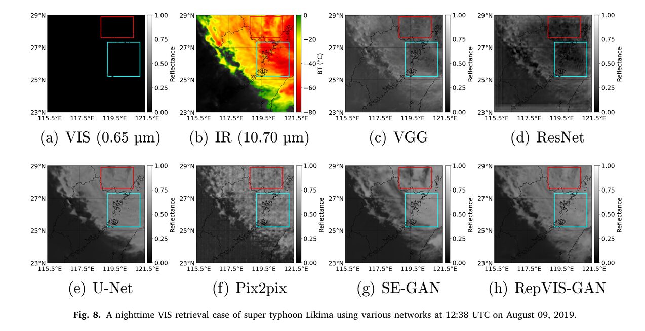
The complete study — including the Super Typhoon Likima case study, full-China nighttime VIS retrieval results at three time steps, generalization tests on 2023 data and the SEN1-2 SAR-optical benchmark, and detailed ablation tables across component, convolution, and attention configurations — is published in the ISPRS Journal of Photogrammetry and Remote Sensing.
Si, J., Li, C., & Han, L. (2026). RepVIS-GAN: A reparameterized GAN-based network for visible image retrieval from geostationary satellite infrared observations. ISPRS Journal of Photogrammetry and Remote Sensing, 236, 162–174. https://doi.org/10.1016/j.isprsjprs.2026.03.025
This article is an independent editorial analysis of peer-reviewed research. The PyTorch implementation is an educational adaptation; the original paper used the TensorFlow framework. Loss weights λ1=1, λ2=λ3=5, λ4=λ5=0.5 match the paper exactly. Image patches are 600×600 pixels at 1km resolution for FY-4A; the smoke test uses 64×64 for CPU feasibility. Supported by the National Natural Science Foundation of China (Grant 42275003).