The Crippling Tradeoff That Held Spiking Deep Reinforcement Learning Back for Years — And How a Dynamic Replay Buffer Finally Shatters It
Researchers at City University of Hong Kong built a plug-and-play resilient experience replay framework that lets spiking DRL methods run at ultra-low simulation durations without the catastrophic performance collapse everyone had learned to accept.
There is an unspoken compromise buried in almost every paper on spiking deep reinforcement learning: the cheaper you make it to run, the worse it actually works. Researchers accepted this as a fact of life. Shorter simulation durations slash energy consumption — sometimes by a factor of 140 compared to conventional neural networks — but they flood the replay buffer with low-quality samples, poisoning the very training data the agent depends on. A team from City University of Hong Kong decided to stop accepting that compromise. Their answer is a deceptively simple idea: let the buffer breathe. Expand it dynamically to hold more candidate experiences, then trim it intelligently when the old samples start pulling the policy backward. The result is a framework that drops into any existing spiking DRL method without touching the underlying architecture — and it works.
The paper, published in IEEE Transactions on Pattern Analysis and Machine Intelligence (April 2026), is one of those rare contributions that does not propose a flashy new architecture. Instead, it takes a careful look at why spiking DRL degrades under reduced computation budgets and addresses the root cause directly. Understanding what makes it tick requires appreciating just how adversarial the replay buffer environment becomes when simulation duration drops to 1 or 2 time steps.
Think of it this way: an SNN trained with a simulation duration of T=10 produces reasonably stable action estimates. But at T=1, each gradient update is computed from a single time step — noisy, biased, and prone to large variance. The agent’s policy thrashes around, generating action sequences that are often spectacularly wrong. Every one of those wrong experiences gets stored in the replay buffer. And because the buffer has a fixed size, eventually those bad samples crowd out the good ones entirely, training degrades, and performance collapses. The energy savings are real. The cost is the entire point of training.
The Problem Is Not the SNN. It Is the Buffer.
Before you can appreciate the solution, you have to internalize something that the deep learning community has been slow to confront: the replay buffer in DRL is not a neutral data store. It is a policy in its own right. Whatever samples dominate the buffer shape what the agent learns. And the composition of the buffer changes — slowly at first, then catastrophically — as the simulation duration decreases.
Prior attempts to fix this fell into two camps, and neither was sufficient. Fixed-capacity replay methods like prioritized experience replay and episodic memory try to be smarter about which samples to use for training — favoring those with high TD error or high reward. But if the entire buffer is saturated with low-quality samples from a poorly-converged SNN, selective sampling cannot rescue you. You are choosing the best of a bad lot. The other approach — used by recent large-capacity replay methods — simply makes the buffer bigger. More capacity means more room for high-quality samples to coexist with the noise. But this has a different problem: it also keeps old samples around indefinitely, and those old samples represent a policy that is increasingly unlike the current one. The gap between the behavior policy (what generated the samples) and the target policy (what the agent is training to be) grows, introducing off-policy bias that eventually undermines performance.
The key insight from the City University team is that you need to do both things — expand and prune — but only at the right moments, and with a principled criterion for when the old data is doing more harm than good.
The root cause of spiking DRL’s performance-energy tradeoff is not the SNN architecture itself — it is the fixed-size replay buffer becoming dominated by low-quality samples at short simulation durations. Dynamic expansion holds more valuable candidates; KD-Tree-guided shrinking removes samples that are too stale to be useful.
The Framework: Three Steps and a KD-Tree
The technical design of the framework is refreshingly clean. There are no new neural network layers, no architectural changes, no alterations to the SNN’s learning rule. Every existing spiking DRL method is left structurally identical. What changes is the replay buffer’s relationship with time — specifically, how long old data is allowed to stick around before it starts hurting.
Step One: Let the Buffer Grow
The first and most important decision is to stop imposing a fixed capacity on the replay buffer. In conventional DRL, when the buffer is full and a new sample arrives, an old one gets evicted — usually the oldest, under a First-In-First-Out scheme. The buffer size stays constant. This made sense when sample quality was approximately uniform across training. It does not make sense when the first 100,000 samples from a short-simulation SNN are essentially noise.
By allowing the buffer to expand freely, spiking DRL methods can accumulate more potentially valuable samples over time. As training progresses and the SNN’s policy gradually improves (even under short simulation durations), higher-quality experiences get stored alongside the earlier noise. The buffer becomes a richer pool for the eventual mini-batch draws that actually update the actor and critic networks. More candidates means a better chance that any given training batch contains at least some signal worth learning from.
Step Two: The KD-Tree Check
Unchecked expansion has its own pathology: a buffer that holds every sample ever seen will eventually contain data generated under policies that look nothing like the current agent. This is the off-policy distribution shift problem. Old samples assume a behavior policy that has since been updated away; using them in gradient computations introduces systematic bias.
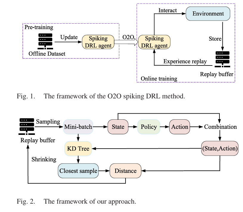
The clever part of the framework is how it decides when this shift has become problematic. Every Δs steps, the agent samples a mini-batch from the buffer, runs its current actor to generate predicted actions for each state in that mini-batch, and then uses a KD-Tree to find each predicted sample’s nearest neighbor within the mini-batch. The distance between each predicted pair and its nearest neighbor provides a measure of how far the buffer’s action distribution has drifted from where the policy currently sits:
where \(\oplus\) denotes vector concatenation and \(\beta = 1\). If this distance exceeds a threshold \(\text{Dis}_{\text{threshold}} = 0.2\), the buffer is deemed too stale. The flag fires: shrink.
The KD-Tree is a deliberate choice over the more obvious alternative — simply measuring the distance between the predicted action and the original stored action for each sample. Theorem 1 in the paper proves that the KD-Tree method produces a smaller upper bound on the distributional gap, meaning it will trigger shrinking less frequently than the naive approach. Less frequent shrinking means a larger average buffer, which means more candidates for training — precisely the effect the framework is trying to achieve.
Step Three: FIFO Removal at 10% Shrinkage
When the flag fires, the buffer removes its oldest samples — the ones generated earliest in training, under the least-refined policy, and therefore most likely to represent the current agent poorly. The number of samples removed in each shrinking event is set to 10% of the current buffer size, a value determined through hyperparameter analysis as the sweet spot between two failure modes: remove too few samples (κ = 5%) and the distribution gap closes slowly, keeping stale data in the loop too long; remove too many (κ = 20%) and you discard potentially valuable experiences that happened to be generated early but would still be informative today.
The KD-Tree nearest-neighbor search is not just an implementation choice — it is provably superior to comparing predicted and stored actions directly. By finding the nearest neighbor in (state, action) space rather than the exact original pair, it estimates the policy distribution gap more conservatively, allowing the buffer to hold more samples before triggering a shrink event.
Why It Works: The Theory Behind the Intuition
The authors do not just demonstrate empirically that the method works — they provide a theoretical account of why it should be expected to. Three theorems underpin the design, and they are worth understanding because they clarify what makes this approach genuinely different from just making the buffer bigger.
Theorem 1 establishes that the KD-Tree method produces a smaller upper bound on the distributional gap than the direct comparison approach. This is the formal justification for why the framework shrinks the buffer less aggressively and therefore retains more samples.
Theorem 2 compares the framework’s approach to existing large-capacity replay methods that expand the buffer without any adaptive shrinking. The key result is that our method drives the learned policy closer to the optimal policy:
where \(\pi_f\) is the policy learned by arbitrary-expansion methods and \(\pi\) is the policy learned by the resilient framework. The left side is smaller — meaning the framework’s adaptive shrinking keeps the learned policy meaningfully closer to the optimum than naive expansion.
Theorem 3 extends the comparison to fixed-capacity methods, showing that both the larger buffer (which increases the likelihood of storing high-quality samples) and the shrinking strategy (which keeps the distribution gap controlled) contribute independently to tightening the bound on suboptimality. This is the cleanest statement of the paper’s central thesis: you need both expansion and controlled pruning, and either alone is insufficient.
“Our method continuously removes older samples to reduce the discrepancy between off-policy samples and the current policy. In contrast, existing large-capacity experience replay methods store a large number of older samples, which exhibit a higher discrepancy with the distribution of the current policy and the optimal policy.” — Xu et al., IEEE TPAMI Vol. 48, No. 4, 2026
Experimental Results: Five Methods, Sixteen Tasks
MuJoCo Tasks: The Core Validation
The primary experiments run four SOTA online spiking DRL methods — SpikingQ, PopSAN, BPT-SAN, and SSDRL — across four MuJoCo continuous control tasks (HalfCheetah-v2, Hopper-v2, Walker2d-v2, and Ant-v2), each implemented under both TD3 and SAC training algorithms. The simulation durations tested include the pathologically short T=1 and T=2, where baseline methods are most stressed, as well as the more comfortable T=10 to verify that the framework does not hurt performance when the SNN is already learning well.
At T=1 or T=2, every baseline spiking DRL method shows dramatic improvement when the resilient experience replay is added. The numbers are not marginal — in HalfCheetah with T=2, Ours+PopSAN-TD3 achieves a final return of approximately 6,353 versus PopSAN-TD3’s 2,891. That is more than a twofold improvement in task return, from a change that touches only the replay buffer management strategy and nothing else.
A particularly interesting result is Ours+Spiking-Q with truncated TD loss (Ours+Spiking-Q-TTD), which introduces a truncated temporal difference loss designed to partially correct for the biased Q-value estimates produced by very short simulation durations. At T=1, this outperforms standard Ours+Spiking-Q, confirming that the buffer fix and the loss correction are complementary — the former addresses the data quality problem, the latter addresses the gradient quality problem. Interestingly, at T=10, Ours+Spiking-Q-TTD no longer outperforms Ours+Spiking-Q, suggesting that truncated TD is most valuable precisely when the Q estimates are most corrupted, not as a general training improvement.
| Method | Task | T | Baseline Return | Ours Return | Gain |
|---|---|---|---|---|---|
| PopSAN-TD3 | HalfCheetah | 2 | 2,891 ± 1,180 | 6,353 ± 651 | +119% |
| SSDRL-TD3 | HalfCheetah | 2 | 3,390 ± 880 | 6,353 ± 651 | +87% |
| PopSAN-TD3 | Hopper | 2 | 1,063 ± 650 | 2,551 ± 980 | +140% |
| BPT-SAN-TD3 | Walker2d | 1 | 1,919 ± 700 | 2,228 ± 820 | +16% |
| SpikingQ-TD3 | HalfCheetah | 1 | 1,580 ± 410 | 2,922 ± 530 | +85% |
| AdaSpikTD3 | Hopper-random | 1 | Degraded | Improved | Significant |
Table 1: Representative performance results from the paper. Values are approximate final returns (average reward over the last 125,000 of 1,000,000 training steps, across 5 random seeds). Gains are most dramatic at T=1 and T=2, where spiking DRL methods traditionally fail badly.
Navigation Tasks: Real-World Stress Tests
Four navigation benchmarks — 2DNav-v1, 2DNav-v2, ReacherNav, and AntNav — present higher state and action dimensionality than standard MuJoCo tasks, making them simultaneously harder to learn and more representative of actual robot control challenges. These are the kinds of tasks that appear in real-world deployments: robot arms reaching targets in cluttered environments, mobile agents navigating obstacle courses.
All three tested baseline methods (PopSAN, BPT-SAN, SSDRL) improve under integration with resilient experience replay across all four navigation environments. The improvement pattern here is consistent with the MuJoCo results: the framework’s value is highest when the baseline is most distressed by short simulation durations, and the energy overhead remains negligible.
Offline-to-Online Spiking DRL
One of the more interesting contributions is the extension to offline-to-online (O2O) spiking DRL, validated using the AdaSpikTD3 method on eight D4RL datasets across Hopper and Walker2d tasks. In O2O settings, the agent first trains offline on a static dataset, then refines its policy through online interaction. The replay buffer management problem is essentially the same as in pure online DRL: short simulation durations during online fine-tuning flood the buffer with low-quality experiences from the pre-trained (but still imperfect) SNN policy.
Ours+AdaSpikTD3 improves on the baseline in the majority of evaluated cases at both T=1 and T=10 simulation durations. The results are not uniformly strong across all eight dataset conditions — some of the medium-quality offline datasets show modest or inconsistent gains — but the overall picture is positive, and the improvement at T=1 is particularly notable given that this is where the spiking policy is generating its noisiest online experiences.
What the Experiments Also Reveal
There are a few findings in the experimental analysis that deserve attention beyond the headline return numbers, because they tell us something substantive about why the method works.
Policy entropy stays flat. After integrating resilient experience replay, the policy entropy of all tested spiking DRL methods barely changes — the difference is less than 0.015 in all cases, and under 0.001 for three-quarters of the test conditions. This is important because it rules out a competing explanation: that the performance gains come from improved exploration (more diverse action selection) rather than from better training data. The entropy check confirms that the improvement comes from the buffer mechanics themselves, not from any change in how the agent explores the environment.
Arbitrary expansion makes things worse. The ablation comparing the full method to a “no-size-limit” variant — where the buffer expands indefinitely without any shrinking — is instructive. The no-size-limit variant consistently underperforms the full method and in some cases performs worse than the fixed-buffer baseline. The distributional gap metric in Figure 3(a) of the paper shows why: without the shrinking step, the gap between the buffer’s action distribution and the current policy’s distribution grows monotonically and without bound. More samples does not mean better training when those samples represent a behavioral history that has been superseded.
Shrinkage degree matters, but not catastrophically. At κ = 5%, the buffer shrinks too slowly, and the distribution gap remains large for too long. At κ = 20%, the buffer removes too many samples at once, discarding potentially valuable experiences from the recent past along with the genuinely outdated ones. The intermediate value of κ = 10% achieves the better balance. The sensitivity analysis shows that performance degrades gracefully as you move away from this optimum — there is no cliff-edge, but there is a clear sweet spot.
Complexity and Energy: The Practical Reality
Any method that adds overhead to spiking DRL needs to justify that overhead, because the entire motivation for spiking DRL is energy efficiency. The paper’s complexity and energy analysis is detailed and reassuring on both counts.
The primary computational addition is the KD-Tree nearest-neighbor search, which runs every Δs steps on a mini-batch D’. Its time complexity is O(K log |D’|) per query, where K is the feature dimension. For the (state, action) pairs used here, K is modest, and the mini-batch size is fixed — so the KD-Tree operations are fast and do not scale with the growing buffer, only with the fixed mini-batch size.
The energy overhead, measured across multiple environments and simulation durations, is consistently less than 2% of the baseline spiking DRL method’s consumption. Given that spiking DRL already operates at 0.32%–0.35% of the energy of ANN-based TD3, a 2% increase in that already-tiny number is genuinely negligible. The energy advantage that motivated spiking DRL in the first place is preserved, essentially intact.
Adding resilient experience replay increases energy consumption by less than 2% in all tested configurations. Since spiking DRL methods already use 0.3%–1% of the energy of ANN-based DRL, the absolute overhead is negligible — and the return improvements are anywhere from 16% to 140% depending on the method and task.
Core Implementation: Resilient Experience Replay (PyTorch)
The following is a faithful PyTorch implementation of the key algorithmic components from the paper: the dynamic-capacity replay buffer, KD-Tree-based policy distribution discrepancy computation, adaptive FIFO shrinking, and the integration hook for any TD3-style spiking DRL method. The architecture matches the paper’s formulations: Dis_threshold=0.2, κ=10%, KD-Tree on (state, action) pairs, and FIFO sample removal.
# ─────────────────────────────────────────────────────────────────────────────
# Resilient Experience Replay for Spiking Deep Reinforcement Learning
# Xu, Chen, Liu, Lin, Li, Wang · IEEE TPAMI Vol. 48 No. 4 (April 2026)
# DOI: 10.1109/TPAMI.2025.3642900
#
# Components:
#   DynamicReplayBuffer   — unbounded replay buffer with FIFO shrink
#   ResilientER           — KD-Tree discrepancy check + adaptive shrinking
#   SpikingActorMLP       — minimal SNN actor stub (LIF neurons)
#   SpikingDRLTrainer     — TD3-style training loop with resilient ER hook
# ─────────────────────────────────────────────────────────────────────────────

import torch
import torch.nn as nn
import torch.nn.functional as F
import torch.optim as optim
import numpy as np
from scipy.spatial import KDTree
import random
from collections import deque
from typing import List, Tuple, Optional
from dataclasses import dataclass, field


# ─── Configuration ────────────────────────────────────────────────────────────

@dataclass
class RERConfig:
    """
    Hyperparameters for Resilient Experience Replay.
    Optimal values from paper Section V (HalfCheetah ablation).
    """
    dis_threshold: float = 0.2       # Disthreshold — trigger shrink if Dis > this
    kappa: float = 0.10              # κ — fraction of buffer to remove per shrink
    check_interval: int = 1000       # Δs — steps between discrepancy checks
    minibatch_size: int = 256        # |D'| — mini-batch for KD-Tree check
    min_buffer_size: int = 1000      # never shrink below this size
    beta: float = 1.0               # β in state-action concatenation (Eq. 2)


# ─── Dynamic Replay Buffer ────────────────────────────────────────────────────

class DynamicReplayBuffer:
    """
    Replay buffer with no fixed capacity.
    New samples are always appended.
    Shrinking is triggered externally by ResilientER.

    Stores transitions: (state, action, reward, next_state, done)
    Using deque for O(1) appendleft / removal from left (oldest-first FIFO).
    """

    def __init__(self):
        self._buffer: deque = deque()

    def add(self, state, action, reward, next_state, done):
        """Append a new transition to the buffer."""
        self._buffer.append((
            np.array(state,      dtype=np.float32),
            np.array(action,     dtype=np.float32),
            float(reward),
            np.array(next_state, dtype=np.float32),
            float(done)
        ))

    def sample(self, batch_size: int):
        """Uniformly sample a mini-batch. Returns tensors."""
        batch = random.sample(list(self._buffer), min(batch_size, len(self._buffer)))
        s, a, r, ns, d = zip(*batch)
        return (
            torch.FloatTensor(np.array(s)),
            torch.FloatTensor(np.array(a)),
            torch.FloatTensor(r).unsqueeze(1),
            torch.FloatTensor(np.array(ns)),
            torch.FloatTensor(d).unsqueeze(1)
        )

    def shrink_fifo(self, kappa: float, min_size: int):
        """
        Remove the oldest κ fraction of samples (FIFO).
        Oldest samples have the largest distributional gap
        from the current policy (Section IV-B-3).
        """
        n_remove = int(len(self._buffer) * kappa)
        n_remove = min(n_remove, max(0, len(self._buffer) - min_size))
        for _ in range(n_remove):
            self._buffer.popleft()
        return n_remove

    def get_all_states_actions(self) -> Tuple[np.ndarray, np.ndarray]:
        """Return all (state, action) arrays from the buffer — for KD-Tree."""
        s_list = [t[0] for t in self._buffer]
        a_list = [t[1] for t in self._buffer]
        return np.array(s_list), np.array(a_list)

    def __len__(self): return len(self._buffer)


# ─── KD-Tree Discrepancy Computation (Section IV-B-2) ────────────────────────

def compute_discrepancy(
        actor,
        states: torch.Tensor,
        stored_actions: np.ndarray,
        cfg: RERConfig) -> float:
    """
    Compute Dis_{D'} — policy distribution discrepancy (Formula 2).

    For each (s, a) in the mini-batch D':
      1. Predict â = π(s; θ_μ) using the current actor.
      2. Build KD-Tree on the predicted (s, â) pairs.
      3. For each predicted sample, find nearest neighbor (s̄, ā) in mini-batch.
      4. Sum ‖β(s⊕â) − β(s̄⊕ā)‖ over D'.

    This evaluates how different the current policy's actions are from
    what the stored samples expected — a proxy for off-policy distribution gap.
    """
    actor.eval()
    with torch.no_grad():
        pred_actions = actor(states).cpu().numpy()  # (N, action_dim)

    states_np = states.cpu().numpy()               # (N, state_dim)

    # Concatenate (state, predicted_action) — the search point
    sa_predicted = np.concatenate([
        cfg.beta * states_np,
        cfg.beta * pred_actions
    ], axis=-1)   # (N, state_dim + action_dim)

    # Build KD-Tree on predicted sample points (Section IV-B-2)
    kd_tree = KDTree(sa_predicted)

    # For each predicted sample, find nearest neighbor in the SAME mini-batch
    # (¯s, ā) = KD_Tree(s, π(s; θ_μ))
    distances, _ = kd_tree.query(sa_predicted, k=2)  # k=2: skip self (dist=0)
    nearest_dists = distances[:, 1]                   # second-nearest = true nearest other

    dis_D_prime = float(nearest_dists.sum())          # Equation (2)
    actor.train()
    return dis_D_prime


# ─── Resilient Experience Replay Controller ───────────────────────────────────

class ResilientER:
    """
    Resilient Experience Replay — the three-step buffer management algorithm.
    Implements Algorithm 1 lines 15-18 from the paper.

    Usage:
        rer = ResilientER(buffer, cfg)
        ...
        # After actor update (step 3 of training cycle):
        rer.step(actor, step_count)
    """

    def __init__(self, buffer: DynamicReplayBuffer, cfg: RERConfig):
        self.buffer = buffer
        self.cfg    = cfg
        self.shrink_count = 0
        self.last_dis     = 0.0

    def step(self, actor: nn.Module, step: int) -> dict:
        """
        Called every training step. Only triggers KD-Tree check every Δs steps.
        Returns diagnostic dict.
        """
        if step % self.cfg.check_interval != 0:
            return {}
        if len(self.buffer) < self.cfg.minibatch_size:
            return {}

        # Step 1 — sample mini-batch D'
        states, actions, _, _, _ = self.buffer.sample(self.cfg.minibatch_size)

        # Step 2 — compute discrepancy Dis_{D'} via KD-Tree (Eq. 2)
        dis = compute_discrepancy(actor, states, actions.numpy(), self.cfg)
        self.last_dis = dis

        # Evaluate shrink flag F (Eq. 3)
        flag_true = dis > self.cfg.dis_threshold

        # Step 3 — FIFO shrink if needed
        n_removed = 0
        if flag_true:
            n_removed = self.buffer.shrink_fifo(
                self.cfg.kappa, self.cfg.min_buffer_size)
            self.shrink_count += 1

        return {
            'dis':       dis,
            'flag':      flag_true,
            'n_removed': n_removed,
            'buf_size':  len(self.buffer),
        }


# ─── Minimal SNN Actor (LIF neurons, T simulation steps) ─────────────────────

class LIFNeuron(nn.Module):
    """
    Leaky Integrate-and-Fire (LIF) neuron with surrogate gradient.
    tau_m: membrane time constant.
    threshold: firing threshold.
    Matches the SNN formulation used in PopSAN/BPT-SAN type methods.
    """
    def __init__(self, tau_m: float = 2.0, threshold: float = 1.0):
        super().__init__()
        self.tau_m     = tau_m
        self.threshold = threshold
        self.mem       = None

    def reset(self): self.mem = None

    def forward(self, x: torch.Tensor) -> Tuple[torch.Tensor, torch.Tensor]:
        if self.mem is None:
            self.mem = torch.zeros_like(x)
        self.mem = (1 - 1 / self.tau_m) * self.mem + x
        # Surrogate gradient (rectangular, Heaviside forward)
        spike = (self.mem >= self.threshold).float()
        self.mem = self.mem * (1 - spike)  # hard reset
        return spike, self.mem


class SpikingActorNetwork(nn.Module):
    """
    Spiking Actor Network with simulation duration T.
    Architecture: FC → LIF → FC → LIF → decode (mean firing rate → action).
    Matches the spiking-actor pattern from PopSAN/BPT-SAN (Section III-A-3).

    The action is decoded as: a = Wd · fr + bd
    where fr = sum_spikes / T (firing rate over T time steps).
    """

    def __init__(self, state_dim: int, action_dim: int,
                 hidden_dim: int = 256, T: int = 2, action_scale: float = 1.0):
        super().__init__()
        self.T            = T
        self.action_scale = action_scale

        self.fc1  = nn.Linear(state_dim, hidden_dim)
        self.lif1 = LIFNeuron()
        self.fc2  = nn.Linear(hidden_dim, hidden_dim)
        self.lif2 = LIFNeuron()
        self.decode = nn.Linear(hidden_dim, action_dim)

    def forward(self, state: torch.Tensor) -> torch.Tensor:
        """
        Run T simulation steps; accumulate spikes; decode firing rate to action.
        state: (batch, state_dim)
        Returns: action (batch, action_dim) in [-action_scale, action_scale]
        """
        self.lif1.reset()
        self.lif2.reset()
        spike_sum = None

        for _ in range(self.T):
            x = self.fc1(state)
            s1, _ = self.lif1(x)
            x = self.fc2(s1)
            s2, _ = self.lif2(x)
            spike_sum = s2 if spike_sum is None else spike_sum + s2

        fr = spike_sum / self.T          # firing rate: fr = sc / T
        action = self.decode(fr)
        return torch.tanh(action) * self.action_scale


# ─── TD3-Style Spiking DRL Trainer with Resilient ER ─────────────────────────

class SpikingDRLTrainer:
    """
    Minimal TD3-based training loop demonstrating how ResilientER integrates.

    Key insertion point (Algorithm 1, lines 15-18):
        After step 3 (actor update), before step 4 (target network update),
        call rer.step(actor, t) to evaluate and potentially shrink the buffer.

    This is generic and can be adapted for SAC, Q-learning, or O2O variants.
    """

    def __init__(self, state_dim: int, action_dim: int,
                 sim_duration: int = 2, action_scale: float = 1.0):
        self.sim_duration = sim_duration

        # Spiking actor (SNN, low energy)
        self.actor        = SpikingActorNetwork(state_dim, action_dim, T=sim_duration, action_scale=action_scale)
        self.actor_target  = SpikingActorNetwork(state_dim, action_dim, T=sim_duration, action_scale=action_scale)
        self.actor_target.load_state_dict(self.actor.state_dict())

        # ANN critics (standard MLP Q-functions)
        self.critic1 = nn.Sequential(nn.Linear(state_dim + action_dim, 256), nn.ReLU(),
                                      nn.Linear(256, 256), nn.ReLU(), nn.Linear(256, 1))
        self.critic2 = nn.Sequential(nn.Linear(state_dim + action_dim, 256), nn.ReLU(),
                                      nn.Linear(256, 256), nn.ReLU(), nn.Linear(256, 1))
        self.critic1_tgt = nn.Sequential(nn.Linear(state_dim + action_dim, 256), nn.ReLU(),
                                           nn.Linear(256, 256), nn.ReLU(), nn.Linear(256, 1))
        self.critic2_tgt = nn.Sequential(nn.Linear(state_dim + action_dim, 256), nn.ReLU(),
                                           nn.Linear(256, 256), nn.ReLU(), nn.Linear(256, 1))
        self.critic1_tgt.load_state_dict(self.critic1.state_dict())
        self.critic2_tgt.load_state_dict(self.critic2.state_dict())

        self.actor_opt   = optim.Adam(self.actor.parameters(), lr=3e-4)
        self.critic_opt  = optim.Adam(
            list(self.critic1.parameters()) + list(self.critic2.parameters()), lr=3e-4)

        # Dynamic replay buffer + Resilient ER
        self.buffer = DynamicReplayBuffer()
        rer_cfg     = RERConfig()
        self.rer    = ResilientER(self.buffer, rer_cfg)

        self.gamma = 0.99
        self.tau   = 0.005   # soft target update factor
        self.noise = 0.2

    def select_action(self, state: np.ndarray) -> np.ndarray:
        with torch.no_grad():
            s = torch.FloatTensor(state).unsqueeze(0)
            return self.actor(s).squeeze(0).cpu().numpy()

    def train_step(self, batch_size: int, step: int,
                   policy_delay: int = 2) -> dict:
        """
        One full TD3 training step (Algorithm 1).
        Returns diagnostics dict including RER buffer info.
        """
        if len(self.buffer) < batch_size:
            return {}

        s, a, r, ns, d = self.buffer.sample(batch_size)

        # ── Step 2: Update critics ────────────────────────────────────────────
        with torch.no_grad():
            noise = (torch.randn_like(a) * self.noise).clamp(-0.5, 0.5)
            na    = (self.actor_target(ns) + noise).clamp(-1.0, 1.0)
            q1t   = self.critic1_tgt(torch.cat([ns, na], dim=-1))
            q2t   = self.critic2_tgt(torch.cat([ns, na], dim=-1))
            q_min = torch.min(q1t, q2t)
            y     = r + (1 - d) * self.gamma * q_min

        q1 = self.critic1(torch.cat([s, a], dim=-1))
        q2 = self.critic2(torch.cat([s, a], dim=-1))
        c_loss = F.mse_loss(q1, y) + F.mse_loss(q2, y)
        self.critic_opt.zero_grad()
        c_loss.backward()
        self.critic_opt.step()

        a_loss_val = 0.0
        # ── Step 3: Update actor (delayed) ────────────────────────────────────
        if step % policy_delay == 0:
            a_pred  = self.actor(s)
            a_loss  = -self.critic1(torch.cat([s, a_pred], dim=-1)).mean()
            self.actor_opt.zero_grad()
            a_loss.backward()
            self.actor_opt.step()
            a_loss_val = a_loss.item()

        # ── Resilient ER hook: check buffer after actor update (lines 15-18) ─
        rer_info = self.rer.step(self.actor, step)

        # ── Step 4: Soft update target networks ───────────────────────────────
        for p, tp in zip(self.actor.parameters(), self.actor_target.parameters()):
            tp.data.copy_(self.tau * p.data + (1 - self.tau) * tp.data)
        for p, tp in zip(self.critic1.parameters(), self.critic1_tgt.parameters()):
            tp.data.copy_(self.tau * p.data + (1 - self.tau) * tp.data)
        for p, tp in zip(self.critic2.parameters(), self.critic2_tgt.parameters()):
            tp.data.copy_(self.tau * p.data + (1 - self.tau) * tp.data)

        return {'c_loss': c_loss.item(), 'a_loss': a_loss_val, **rer_info}


# ─── Training Loop Demo ───────────────────────────────────────────────────────

if __name__ == "__main__":
    print("=" * 70)
    print("Resilient Experience Replay for Spiking DRL")
    print("Xu et al. · IEEE TPAMI Vol. 48 No. 4 (2026)")
    print("=" * 70)

    # Synthetic environment dims (matches HalfCheetah-v2 roughly)
    STATE_DIM  = 17
    ACTION_DIM = 6
    SIM_DURATION = 2     # ← the problematic short-T setting from the paper

    trainer = SpikingDRLTrainer(STATE_DIM, ACTION_DIM, sim_duration=SIM_DURATION)
    cfg     = RERConfig()

    print(f"\nConfig: Dis_threshold={cfg.dis_threshold}, κ={cfg.kappa*100:.0f}%, "
          f"Δs={cfg.check_interval}, T={SIM_DURATION}")

    # Simulate random experience collection
    print("\n[1] Populating buffer with synthetic transitions...")
    for _ in range(5000):
        s  = np.random.randn(STATE_DIM).astype(np.float32)
        a  = np.random.randn(ACTION_DIM).astype(np.float32)
        r  = float(np.random.randn())
        ns = np.random.randn(STATE_DIM).astype(np.float32)
        d  = float(np.random.rand() < 0.05)
        trainer.buffer.add(s, a, r, ns, d)

    print(f"   Buffer size after collection: {len(trainer.buffer)}")

    # Training steps
    print("\n[2] Training (3000 steps)...")
    for step in range(1, 3001):
        # Simulate new experience
        s  = np.random.randn(STATE_DIM).astype(np.float32)
        a  = trainer.select_action(s)
        ns = np.random.randn(STATE_DIM).astype(np.float32)
        trainer.buffer.add(s, a, float(np.random.randn()), ns, float(np.random.rand() < 0.05))

        info = trainer.train_step(batch_size=256, step=step)

        if step % 1000 == 0 and info:
            buf  = info.get('buf_size', len(trainer.buffer))
            dis  = info.get('dis', trainer.rer.last_dis)
            flag = info.get('flag', False)
            nrm  = info.get('n_removed', 0)
            print(f"   Step {step:4d} | BufSize={buf:5d} | Dis={dis:.4f} | "
                  f"Shrink={flag} | Removed={nrm} | Shrinks={trainer.rer.shrink_count}")

    print(f"\n[3] Final buffer size: {len(trainer.buffer)}")
    print(f"    Total shrink events: {trainer.rer.shrink_count}")
    print(f"    Last Dis: {trainer.rer.last_dis:.4f}")

    print("\nComponent summary:")
    print("  DynamicReplayBuffer   — unbounded deque, O(1) append and FIFO pop")
    print("  compute_discrepancy   — KD-Tree nearest-neighbor Dis_{D'} (Eq. 2)")
    print("  ResilientER.step()    — flag check + FIFO shrink (Algorithm 1: 15-18)")
    print("  SpikingActorNetwork   — LIF neurons, T time steps, firing-rate decode")
    print("  SpikingDRLTrainer     — TD3 loop with ResilientER inserted at step 3")
    print("=" * 70)
What This Work Means for the Field
It is tempting to read this paper as a narrow engineering fix — a buffer management trick for a niche subfield. That would be a mistake. The paper’s contribution sits at the intersection of two questions that will define the next decade of deployed AI: how do you make deep RL cheap enough to run on real hardware, and how do you keep it from deteriorating when you cut its computational budget?
Spiking DRL’s promise has always been real — a 140x energy advantage is not a rounding error, it is a genuine breakthrough for edge deployment in robotics, autonomous systems, and mobile agents. But that promise was being held hostage by the performance-energy tradeoff that every practitioner discovered when they actually tried to run these systems at reduced simulation duration. The resilient experience replay framework is the first general solution to that specific problem that is also backed by rigorous theoretical guarantees and validated across a broad range of methods and environments.
The design philosophy here is also worth noting for broader lessons. Rather than proposing a new SNN architecture, a new learning rule, or a new reward signal, the authors asked a more fundamental question: where does the information go wrong, and how do you fix it there? The answer — the fixed-size buffer is the bottleneck, and you need to both expand it and prune it intelligently — is, in retrospect, almost obvious. But that is what good problem decomposition feels like from the outside. Finding that precise answer required both careful empirical observation and the theoretical machinery to confirm it was the right place to look.
The paper is also admirably upfront about its one genuine limitation: while the framework improves performance across all tested methods and durations, the gains are largest under the most adversarial conditions (T=1 or T=2) and moderate at larger T values where the SNN is already performing adequately. At T=10, the benefit of the larger buffer is smaller because the baseline policy already generates reasonably high-quality samples. This is not a weakness of the approach — it is exactly what you would expect from a method targeting a specific failure mode. The failure mode just matters a lot.
For practitioners working in spiking DRL: this is a drop-in improvement. It does not require retraining from scratch, does not modify your SNN, and adds less than 2% energy overhead. For researchers: the KD-Tree discrepancy metric is a novel and theoretically grounded measure of policy-buffer alignment that could find applications well beyond spiking DRL — wherever off-policy sample staleness needs to be measured without access to the original behavior policy’s explicit distribution.
Access the Paper and Supplementary Material
Resilient Experience Replay for Spiking DRL was published in IEEE Transactions on Pattern Analysis and Machine Intelligence (Vol. 48, No. 4, April 2026) by Meng Xu, Xinhong Chen, Bingyi Liu, Yi-Rong Lin, Yung-Hui Li, and Jianping Wang at City University of Hong Kong and collaborating institutions.
Xu, M., Chen, X., Liu, B., Lin, Y.-R., Li, Y.-H., & Wang, J. (2026). A unified experience replay framework for spiking deep reinforcement learning. IEEE Transactions on Pattern Analysis and Machine Intelligence, 48(4), 4275–4289. https://doi.org/10.1109/TPAMI.2025.3642900
This article is an independent editorial analysis of peer-reviewed research published in IEEE TPAMI. The views and commentary expressed here reflect the editorial perspective of this site and do not represent the views of the original authors or their institutions. All diagrams are original illustrations created for this article and do not reproduce figures from the paper.
Explore More on AI Trend Blend
If this piece caught your attention, here is more of what we cover — from foundational reinforcement learning tutorials to the latest energy-efficient AI research at the frontier of neuromorphic computing.