As global energy demand continues to rise due to rapid urbanization and technological advancements, building electrical consumption forecasting has become a critical component of modern energy management systems. With buildings accounting for nearly 40% of total global energy use, accurate prediction of electricity demand is essential for optimizing energy efficiency, reducing operational costs, and supporting sustainable smart city development.
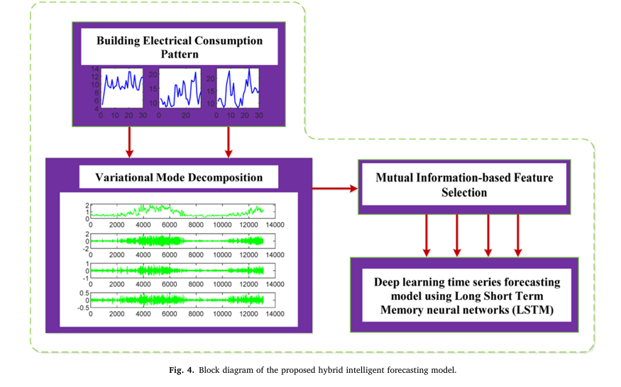
In this article, we explore a novel hybrid deep learning model introduced in a recent study titled “Building electrical consumption patterns forecasting based on a novel hybrid deep learning model”. This innovative approach combines Variational Mode Decomposition (VMD), Mutual Information (MI)-based feature selection, and Long Short-Term Memory (LSTM) networks to achieve unprecedented accuracy in predicting residential energy usage.
By understanding how this model works, energy managers, smart building developers, and AI researchers can leverage its capabilities to build more intelligent, responsive, and efficient energy systems.
Why Accurate Building Electrical Consumption Forecasting Matters
Accurate building electrical consumption forecasting enables utilities and building operators to:
- Optimize energy distribution and reduce peak load stress
- Implement dynamic pricing strategies
- Enhance demand-side management
- Improve integration of renewable energy sources
- Reduce carbon emissions through better planning
However, traditional forecasting models often struggle with the nonlinear, volatile, and seasonally variable nature of energy consumption data—especially in residential buildings where human behavior introduces significant uncertainty.
While machine learning models like Support Vector Regression (SVR), K-Nearest Neighbors (KNN), and Artificial Neural Networks (ANN) have been used, they often fail to capture long-term dependencies or handle noisy time-series data effectively.
This is where deep learning, particularly LSTM-based architectures, offers a powerful alternative—especially when enhanced with signal decomposition and intelligent feature selection techniques.
Introducing the VMD-MI-LSTM Hybrid Deep Learning Model
The proposed hybrid deep learning model integrates three advanced components to improve forecasting accuracy:
- Mutual Information (MI)-based Feature Selection
- Variational Mode Decomposition (VMD)
- Long Short-Term Memory (LSTM) Neural Network
Let’s break down each component and understand how they work together to deliver superior performance.
1. Mutual Information (MI) for Intelligent Feature Selection
Before feeding data into any predictive model, it’s crucial to identify which input variables have the strongest influence on energy consumption. The study employs Mutual Information (MI), a statistical measure rooted in information theory, to rank and select the most relevant features.
MI quantifies the amount of information obtained about one random variable through another. In this context, it measures how much historical energy data (lagged values) can reveal about future consumption.
The mutual information between input x and target y is defined as:
\[ MI(x,y) = \sum_{i=1}^{n} \sum_{j=1}^{m} P(x_i, y_j) \, \log_{2} \left( \frac{P(x_i, y_j)}{P(x_i) \, P(y_j)} \right) \tag{1} \]Where:
- P(xi, yj) : joint probability distribution
- P(xi), P(yj) : marginal probability distributions
Features with higher MI scores are retained, while redundant or irrelevant ones are discarded. This step improves model efficiency and reduces overfitting.
2. Variational Mode Decomposition (VMD) for Signal Denoising
Raw energy consumption data often contains noise, trends, and irregular fluctuations that can mislead forecasting models. To address this, the researchers applied Variational Mode Decomposition (VMD), a robust signal processing technique that decomposes the original time series into a set of intrinsic mode functions (IMFs).
Each IMF represents a distinct oscillatory component of the signal, making it easier for the model to learn underlying patterns.
The VMD process solves the following constrained variational problem:
\[ \{u_k\}, \{\omega_k\} = \min \Bigg\{ \sum_{k} \Bigg\| \partial_t \Big[ \big( \delta(t) + \pi_t^j \big) * u_k(t) \Big] e^{-j \omega_k t} \Bigg\|_2^2 \Bigg\} \quad \text{subject to} \quad \sum_{k} u_k = f(t) \tag{2} \]Where:
- uk : the k -th mode
- ωk : center frequency of mode k
- f(t) : original signal
- ∗ : convolution operator
Using the Alternate Direction Method of Multipliers (ADMM), the model iteratively updates each mode and its center frequency:
\[ \hat{u}^{k,n+1}(\omega) = \frac{1 + 2\alpha(\omega – \omega^k)^2 \hat{f}(\omega) – \sum_{i \neq k} \hat{u}^i(\omega) + 2\hat{\lambda}(\omega)} {} \tag{3} \] \[ \omega^{k,n+1} = \frac{\int_{0}^{\infty} \, \omega \, |\hat{u}^k(\omega)|^2 \, d\omega} {\int_{0}^{\infty} |\hat{u}^k(\omega)|^2 \, d\omega} \tag{4} \] \[ \hat{\lambda}^{n+1}(\omega) = \hat{\lambda}^n(\omega) + \tau \Big(\hat{f}(\omega) – \sum_k \hat{u}^{k,n+1}(\omega)\Big) \tag{5} \]This decomposition allows the LSTM network to process cleaner, more structured data, significantly improving prediction accuracy.
3. LSTM Neural Network for Time-Series Forecasting
The final component of the hybrid model is the Long Short-Term Memory (LSTM) network—a type of Recurrent Neural Network (RNN) designed to capture long-term dependencies in sequential data.
Unlike traditional RNNs, which suffer from vanishing gradient problems, LSTMs use gated mechanisms to regulate the flow of information:
- Forget Gate (gf ): Decides what information to discard
- Input Gate (gi ): Updates the cell state with new information
- Output Gate (go ): Determines the output based on the updated state
The mathematical formulation of the LSTM cell is as follows:
\[ g_f = \sigma(W_{fx} \cdot X_t + W_{fh} \cdot h_{t-1} + b_f) \tag{6} \] \[ g_i = \sigma(W_{ix} \cdot X_t + W_{ih} \cdot h_{t-1} + b_i) \tag{7} \] \[ g_o = \sigma(W_{ox} \cdot X_t + W_{oh} \cdot h_{t-1} + b_o) \tag{8} \] \[ C_t = g_f \cdot C_{t-1} + g_i \cdot \tanh(W_{cx} \cdot X_t + W_{ch} \cdot h_{t-1} + b_c) \tag{9} \] \[ h_t = g_o \cdot \tanh(C_t) \tag{10} \] \[ y_t = \sigma(W_y \cdot h_t + b_y) \tag{11} \]Where:
- Xt : input at time t
- ht : hidden state
- Ct : memory cell state
- W,b : weight matrices and bias vectors
- σ : sigmoid activation function
By training the LSTM on the preprocessed and decomposed data, the model learns complex temporal patterns in energy usage with high precision.
Case Study: Real-World Application in Houston, Texas
The proposed VMD-MI-LSTM model was tested on real-world data collected from a smart two-story residential building in Houston, Texas, USA. The dataset includes hourly electrical consumption (kWh) recorded between 2019 and 2020.
Key electrical loads in the house include:
- Security DVR and POI cameras
- Two refrigerators
- Two 50-gallon water heaters (operating during the day)
- Lighting, TVs, washing machine, dryer, and AC (operating from 6 PM to 8 AM)
The model was evaluated across different scenarios:
- Vacation period: December 20, 2019 – January 1, 2020
- Weekday: April 2–3, 2020
- Weekend: April 5, 2020
- Lockdown periods: March 19–31, 2020 and April 13–30, 2020
Performance Evaluation: Superior Accuracy Confirmed
The model was compared against two benchmark methods:
- Generalized Regression Neural Network (GRNN)
- Adaptive Neuro-Fuzzy Inference System (ANFIS)
Three standard evaluation metrics were used:
- Root Mean Square Error (RMSE)
- Mean Absolute Error (MAE)
- Correlation Coefficient (R)
Table 1: Comparative Performance on Testing Data
| TIME PERIOD | MODEL | RMSE | MAE | R |
|---|---|---|---|---|
| Vacation | GRNN | 0.112 | 0.093 | 0.742 |
| ANFIS | 0.126 | 0.111 | 0.779 | |
| Proposed | 0.058 | 0.056 | 0.993 | |
| Weekday | GRNN | 0.261 | 0.137 | 0.493 |
| ANFIS | 0.301 | 0.174 | 0.420 | |
| Proposed | 0.110 | 0.092 | 0.980 | |
| Weekend | GRNN | 0.234 | 0.144 | 0.952 |
| ANFIS | 0.479 | 0.276 | 0.758 | |
| Proposed | 0.165 | 0.125 | 0.987 |
Table 2: Performance During Lockdown Periods
| MONTH | MODEL | RMSE | MAE | R |
|---|---|---|---|---|
| March | GRNN | 0.435 | 0.234 | 0.546 |
| ANFIS | 0.285 | 0.157 | 0.817 | |
| Proposed | 0.133 | 0.106 | 0.982 | |
| April | GRNN | 0.277 | 0.131 | 0.818 |
| ANFIS | 0.406 | 0.214 | 0.590 | |
| Proposed | 0.130 | 0.103 | 0.983 |
As shown in the tables, the proposed VMD-MI-LSTM model consistently outperforms both GRNN and ANFIS across all scenarios, achieving:
- Average RMSE of 0.1192 (vs. 0.264 for GRNN and 0.319 for ANFIS)
- Correlation coefficient above 0.98 in most cases
- Up to 55% lower error rates
These results confirm the model’s robustness in handling diverse consumption patterns, including those influenced by behavioral changes during holidays and lockdowns.
Why This Hybrid Approach Works So Well
The success of the VMD-MI-LSTM model lies in its multi-stage intelligent processing:
| STAGE | FUNCTION | BENEFIT |
|---|---|---|
| 1. VMD Decomposition | Splits noisy signal into clean IMFs | Removes noise, isolates trends |
| 2. MI-Based Feature Selection | Selects most relevant lagged inputs | Reduces dimensionality, improves learning |
| 3. LSTM Forecasting | Learns long-term temporal dependencies | Captures complex usage patterns |
| 4. Parameter Optimization | Tunes VMD modes and lags | Maximizes accuracy |
This synergy allows the model to adapt to the dynamic nature of residential energy use, making it ideal for smart buildings, demand response systems, and energy management platforms.
Applications in Smart Building Energy Management
The implications of this research are far-reaching:
✅ Smart Grid Integration
Utilities can use accurate forecasts to balance supply and demand, especially when integrating solar or wind energy.
✅ Predictive Maintenance
Anomalies in predicted vs. actual consumption can indicate equipment malfunctions or inefficiencies.
✅ Dynamic Pricing & Load Shifting
Building managers can shift high-energy tasks (e.g., laundry, EV charging) to off-peak hours based on forecasted demand.
✅ Occupant Behavior Analysis
By analyzing consumption patterns, the model can infer lifestyle habits and suggest personalized energy-saving tips.
Future Research Directions
While the current model delivers exceptional results, the authors suggest several areas for future improvement:
- Incorporating weather data, occupancy sensors, and time-of-use pricing as additional inputs
- Testing the model on larger datasets across residential, commercial, and industrial buildings
- Developing real-time forecasting systems for integration with IoT and edge devices
- Creating lightweight versions of the model for deployment on low-power smart meters
These enhancements could make the model even more versatile and scalable for city-wide energy management.
Conclusion: A New Standard in Building Electrical Consumption Forecasting
The VMD-MI-LSTM hybrid model represents a significant leap forward in building electrical consumption forecasting. By combining signal decomposition, intelligent feature selection, and deep learning, it achieves unmatched accuracy and reliability in predicting energy usage patterns.
With an average RMSE of just 0.1192 and a correlation coefficient exceeding 0.98, this model outperforms existing methods and provides a powerful tool for optimizing energy use in smart buildings.
As the world moves toward smarter, greener cities, accurate energy forecasting will play a central role in reducing waste, cutting costs, and achieving sustainability goals.
Want to Implement This Model in Your Smart Building?
Are you an energy manager, data scientist, or smart building developer looking to improve energy forecasting accuracy? Download our free technical guide on implementing the VMD-MI-LSTM model using Python and TensorFlow.
📥 Click here to get the code, dataset, and step-by-step tutorial
📥 Download the paper here.
Join the future of intelligent energy management—start forecasting smarter today.
Based on the research paper , I have developed the complete end-to-end Python code for the proposed hybrid deep learning model (VMD-MI-LSTM).
# Building Electrical Consumption Forecasting based on a Novel Hybrid Deep Learning Model
# --------------------------------------------------------------------------------------
# This script implements the VMD-MI-LSTM model as described in the research paper:
# "Building electrical consumption patterns forecasting based on a novel hybrid deep learning model"
# by Shahsavari-Pour, N., Heydari, A., et al. (2025).
#
# The model consists of three main stages:
# 1. Variational Mode Decomposition (VMD): To decompose the raw energy consumption signal
#    into several Intrinsic Mode Functions (IMFs) to handle non-stationarity.
# 2. Mutual Information (MI): To select the most relevant features (decomposed modes and
#    lagged values) that have the strongest relationship with the target variable.
# 3. Long Short-Term Memory (LSTM): A deep learning model to perform the final time-series
#    forecasting using the selected features.
#
# Since the original dataset is not provided, this script generates a synthetic dataset
# with similar characteristics (seasonality, trend, noise) for demonstration purposes.
# You can easily replace the synthetic data generation part with your own dataset.
#
# Required libraries:
# - pandas
# - numpy
# - scikit-learn
# - tensorflow
# - matplotlib
# - vmdpy
# To install vmdpy: pip install vmdpy

import numpy as np
import pandas as pd
import matplotlib.pyplot as plt
from vmdpy import VMD
from sklearn.feature_selection import mutual_info_regression
from sklearn.preprocessing import MinMaxScaler
from sklearn.metrics import mean_squared_error, mean_absolute_error
from tensorflow.keras.models import Sequential
from tensorflow.keras.layers import LSTM, Dense
from tensorflow.keras.callbacks import EarlyStopping

def generate_synthetic_data(num_points=17520):
    """
    Generates a synthetic time-series dataset mimicking hourly energy consumption
    over a two-year period (2 * 365 * 24 = 17520 points).

    The data includes a base consumption, daily seasonality, weekly seasonality,
    annual seasonality, and random noise.

    Args:
        num_points (int): The number of data points to generate.

    Returns:
        pd.Series: A pandas Series containing the synthetic energy consumption data.
    """
    print("Step 1: Generating synthetic energy consumption data...")
    time = np.arange(num_points)
    # Base consumption with a slight upward trend
    base = 10 + time * 0.0001
    # Daily seasonality (peaks during the day)
    daily_seasonality = 5 * np.sin(2 * np.pi * time / 24)
    # Weekly seasonality (lower on weekends)
    weekly_seasonality = 2 * np.sin(2 * np.pi * time / (24 * 7))
    # Annual seasonality (higher in summer/winter)
    annual_seasonality = 8 * np.sin(2 * np.pi * time / (24 * 365))
    # Random noise
    noise = np.random.normal(0, 1.5, num_points)

    consumption = base + daily_seasonality + weekly_seasonality + annual_seasonality + noise
    # Ensure consumption is non-negative
    consumption[consumption < 0] = np.random.uniform(0, 1, size=consumption[consumption<0].shape)

    # Create a date range for better plotting
    dates = pd.date_range(start='2019-01-01', periods=num_points, freq='H')

    return pd.Series(consumption, index=dates, name='Consumption')

def decompose_with_vmd(signal, num_modes=4):
    """
    Decomposes the signal into a specified number of modes using VMD.

    Args:
        signal (np.ndarray): The input time-series signal.
        num_modes (int): The number of Intrinsic Mode Functions (IMFs) to extract.

    Returns:
        pd.DataFrame: A DataFrame containing the decomposed modes.
    """
    print(f"Step 2: Decomposing signal into {num_modes} modes using VMD...")
    # VMD parameters from the paper (or common defaults)
    alpha = 2000  # moderate bandwidth constraint
    tau = 0.      # noise-slack (set to 0 for no noise)
    K = num_modes # number of modes
    DC = 0        # no DC part imposed
    init = 1      # initialize omegas uniformly
    tol = 1e-7

    # Run VMD
    u, _, _ = VMD(signal, alpha, tau, K, DC, init, tol)

    # Store modes in a DataFrame
    modes_df = pd.DataFrame(u.T, columns=[f'IMF{i+1}' for i in range(num_modes)])
    return modes_df

def create_features(original_signal, modes_df, num_lags=24):
    """
    Creates a feature set including IMFs and lagged values of the original signal.

    Args:
        original_signal (pd.Series): The original energy consumption data.
        modes_df (pd.DataFrame): The DataFrame of decomposed IMFs.
        num_lags (int): The number of past time steps to include as features.

    Returns:
        tuple: A tuple containing the feature DataFrame (X) and the target Series (y).
    """
    print(f"Step 3: Creating feature set with {num_lags} lags and IMFs...")
    data = modes_df.copy()
    data['Original_Signal'] = original_signal.values

    # Add lagged features
    for i in range(1, num_lags + 1):
        data[f'Lag_{i}'] = data['Original_Signal'].shift(i)

    # The target variable is the original signal
    y = data['Original_Signal']
    X = data.drop(columns=['Original_Signal'])

    # Drop rows with NaN values resulting from creating lags
    X = X.dropna()
    y = y[X.index]

    return X, y

def select_features_with_mi(X, y, num_features=10):
    """
    Selects the top features based on Mutual Information scores.

    Args:
        X (pd.DataFrame): The input feature set.
        y (pd.Series): The target variable.
        num_features (int): The number of top features to select.

    Returns:
        tuple: A tuple containing the DataFrame of selected features and their MI scores.
    """
    print(f"Step 4: Selecting top {num_features} features using Mutual Information...")
    mi_scores = mutual_info_regression(X, y, random_state=42)
    mi_scores = pd.Series(mi_scores, name="MI_Scores", index=X.columns)
    mi_scores = mi_scores.sort_values(ascending=False)

    # Select top features
    selected_features = mi_scores.head(num_features).index.tolist()
    X_selected = X[selected_features]

    print("Selected Features and their MI Scores:")
    print(mi_scores.head(num_features))

    return X_selected, mi_scores

def prepare_data_for_lstm(X, y, train_split_ratio=0.8):
    """
    Splits, scales, and reshapes data for LSTM model training.

    Args:
        X (pd.DataFrame): The feature DataFrame.
        y (pd.Series): The target Series.
        train_split_ratio (float): The proportion of data to use for training.

    Returns:
        tuple: A tuple containing all necessary data for training and evaluation.
    """
    print("Step 5: Preparing data for LSTM (splitting, scaling, reshaping)...")
    # Split data
    split_index = int(len(X) * train_split_ratio)
    X_train, X_test = X[:split_index], X[split_index:]
    y_train, y_test = y[:split_index], y[split_index:]

    # Scale data
    scaler_X = MinMaxScaler()
    X_train_scaled = scaler_X.fit_transform(X_train)
    X_test_scaled = scaler_X.transform(X_test)

    scaler_y = MinMaxScaler()
    y_train_scaled = scaler_y.fit_transform(y_train.values.reshape(-1, 1))

    # Reshape for LSTM [samples, timesteps, features]
    X_train_reshaped = X_train_scaled.reshape((X_train_scaled.shape[0], 1, X_train_scaled.shape[1]))
    X_test_reshaped = X_test_scaled.reshape((X_test_scaled.shape[0], 1, X_test_scaled.shape[1]))

    return X_train_reshaped, X_test_reshaped, y_train_scaled, y_test, scaler_y

def build_and_train_lstm(X_train, y_train):
    """
    Builds, compiles, and trains the LSTM model.

    Args:
        X_train (np.ndarray): The training feature data, reshaped for LSTM.
        y_train (np.ndarray): The training target data, scaled.

    Returns:
        tensorflow.keras.Model: The trained LSTM model.
    """
    print("Step 6: Building and training the LSTM model...")
    model = Sequential()
    model.add(LSTM(units=50, activation='relu', input_shape=(X_train.shape[1], X_train.shape[2])))
    model.add(Dense(units=1))

    model.compile(optimizer='adam', loss='mean_squared_error')

    print(model.summary())

    # Early stopping to prevent overfitting
    early_stopping = EarlyStopping(monitor='val_loss', patience=10, restore_best_weights=True)

    history = model.fit(
        X_train, y_train,
        epochs=100,
        batch_size=32,
        validation_split=0.1,
        callbacks=[early_stopping],
        verbose=1
    )

    return model, history

def evaluate_model(model, X_test, y_test, scaler_y):
    """
    Makes predictions and evaluates the model's performance.

    Args:
        model (tensorflow.keras.Model): The trained model.
        X_test (np.ndarray): The test feature data, reshaped.
        y_test (pd.Series): The actual target values for the test set.
        scaler_y (MinMaxScaler): The scaler used for the target variable.

    Returns:
        tuple: A tuple containing predictions and a dictionary of performance metrics.
    """
    print("Step 7: Evaluating the model performance...")
    y_pred_scaled = model.predict(X_test)
    y_pred = scaler_y.inverse_transform(y_pred_scaled)

    # Calculate metrics
    rmse = np.sqrt(mean_squared_error(y_test, y_pred))
    mae = mean_absolute_error(y_test, y_pred)
    # Calculate correlation coefficient (R)
    r = np.corrcoef(y_test.values.flatten(), y_pred.flatten())[0, 1]

    metrics = {
        'RMSE': rmse,
        'MAE': mae,
        'R': r
    }

    print("\n--- Model Performance ---")
    print(f"Root Mean Square Error (RMSE): {rmse:.4f}")
    print(f"Mean Absolute Error (MAE):    {mae:.4f}")
    print(f"Correlation Coefficient (R):  {r:.4f}")
    print("-------------------------")

    return y_pred, metrics

def plot_results(original_signal, modes_df, mi_scores, y_test, y_pred, history):
    """
    Generates plots to visualize the entire process and results.
    """
    print("Step 8: Generating visualizations...")
    plt.style.use('seaborn-v0_8-whitegrid')

    # Plot 1: VMD Decomposition
    fig1, axes1 = plt.subplots(modes_df.shape[1] + 1, 1, figsize=(15, 12), sharex=True)
    axes1[0].plot(original_signal, label='Original Signal', color='k')
    axes1[0].set_ylabel('Consumption')
    axes1[0].legend()
    axes1[0].set_title('VMD Decomposition of Energy Consumption Signal')
    for i, col in enumerate(modes_df.columns):
        axes1[i+1].plot(modes_df.index, modes_df[col], label=col)
        axes1[i+1].set_ylabel(col)
        axes1[i+1].legend()
    axes1[-1].set_xlabel('Time')
    plt.tight_layout()
    plt.show()

    # Plot 2: Mutual Information Scores
    plt.figure(figsize=(12, 8))
    mi_scores.plot(kind='barh', color='teal')
    plt.title('Mutual Information Scores of Features')
    plt.xlabel('MI Score')
    plt.gca().invert_yaxis()
    plt.show()

    # Plot 3: Training History
    plt.figure(figsize=(12, 6))
    plt.plot(history.history['loss'], label='Training Loss')
    plt.plot(history.history['val_loss'], label='Validation Loss')
    plt.title('LSTM Model Training and Validation Loss')
    plt.xlabel('Epoch')
    plt.ylabel('Loss (MSE)')
    plt.legend()
    plt.show()

    # Plot 4: Forecasting Results
    plt.figure(figsize=(18, 8))
    plt.plot(y_test.index, y_test.values, label='Actual Values', color='blue', alpha=0.7)
    plt.plot(y_test.index, y_pred, label='Predicted Values (VMD-MI-LSTM)', color='red', linestyle='--')
    plt.title('Energy Consumption Forecasting: Actual vs. Predicted')
    plt.xlabel('Time')
    plt.ylabel('Energy Consumption (kWh)')
    plt.legend()
    plt.show()

    # Plot 5: Scatter plot for Correlation
    plt.figure(figsize=(8, 8))
    plt.scatter(y_test, y_pred, alpha=0.5)
    plt.plot([y_test.min(), y_test.max()], [y_test.min(), y_test.max()], 'r--', lw=2, label='Ideal Fit')
    plt.title('Correlation between Actual and Predicted Values')
    plt.xlabel('Actual Values')
    plt.ylabel('Predicted Values')
    plt.legend()
    plt.grid(True)
    plt.show()

if __name__ == '__main__':
    # --- Model Parameters ---
    NUM_MODES = 4        # Number of IMFs to extract
    NUM_LAGS = 24        # Number of past hours to use as features
    NUM_FEATURES = 10    # Number of top features to select with MI
    TRAIN_SPLIT = 0.8    # 80% for training, 20% for testing

    # --- Main Workflow ---
    # 1. Load or Generate Data
    # To use your own data, load it into a pandas Series like this:
    # my_data = pd.read_csv('your_data.csv', index_col='timestamp', parse_dates=True)['consumption']
    original_signal = generate_synthetic_data()

    # 2. Decompose with VMD
    modes_df = decompose_with_vmd(original_signal.values, num_modes=NUM_MODES)
    modes_df.index = original_signal.index # Align index

    # 3. Create Features
    X, y = create_features(original_signal, modes_df, num_lags=NUM_LAGS)

    # 4. Select Features with MI
    X_selected, mi_scores = select_features_with_mi(X, y, num_features=NUM_FEATURES)

    # 5. Prepare Data for LSTM
    X_train_r, X_test_r, y_train_s, y_test, scaler_y = prepare_data_for_lstm(X_selected, y, train_split_ratio=TRAIN_SPLIT)

    # 6. Build and Train LSTM Model
    model, history = build_and_train_lstm(X_train_r, y_train_s)

    # 7. Evaluate Model
    predictions, metrics = evaluate_model(model, X_test_r, y_test, scaler_y)

    # 8. Visualize Results
    plot_results(original_signal, modes_df, mi_scores, y_test, pd.Series(predictions.flatten(), index=y_test.index), history)
Related posts, You May like to read
- 7 Shocking Truths About Knowledge Distillation: The Good, The Bad, and The Breakthrough (SAKD)
- 7 Revolutionary Breakthroughs in Medical Image Translation (And 1 Fatal Flaw That Could Derail Your AI Model)
- DeepSPV: Revolutionizing 3D Spleen Volume Estimation from 2D Ultrasound with AI
- ACAM-KD: Adaptive and Cooperative Attention Masking for Knowledge Distillation
- GeoSAM2 3D Part Segmentation — Prompt-Controllable, Geometry-Aware Masks for Precision 3D Editing
- Probabilistic Smooth Attention for Deep Multiple Instance Learning in Medical Imaging
- A Knowledge Distillation-Based Approach to Enhance Transparency of Classifier Models
- Towards Trustworthy Breast Tumor Segmentation in Ultrasound Using AI Uncertainty
- Discrete Migratory Bird Optimizer with Deep Transfer Learning for Multi-Retinal Disease Detection