CRGenNet: How Satellites Can See Through Clouds by Never Assuming the Sky Is Clear
Researchers at the University of Twente built an image generation network that does what every prior method refused to do — accept that your helper image might also be covered in clouds. CRGenNet fuses Sentinel-1 SAR radar data with contaminated Sentinel-2 optical imagery to synthesize missing scenes, and backs it with a new flood-disaster benchmark that finally reflects real-world messiness.
Satellite optical imagery has a dirty secret that nobody in the deep learning community wanted to talk about: most training datasets assume your auxiliary reference image is cloud-free. In the real world — especially during floods, hurricanes, and other disasters that demand timely satellite observation — clouds don’t politely step aside for the control image. The Zhengzhou flood of July 2021 put this problem in sharp relief: when you need to see the flood extent most urgently, clouds cover both the target and the backup. CRGenNet from University of Twente’s ITC faculty is the first method purpose-built to handle this exact nightmare scenario, and the results show it outperforms every tested baseline when the auxiliary optical data is itself contaminated.
The Problem Nobody Wanted to Admit
Every SAR-optical image fusion paper for cloud removal follows roughly the same recipe: take a cloudy optical image at time t1, pair it with an all-weather SAR image, and optionally a cloud-free optical image from another date, then learn to generate the missing scene. The “cloud-free auxiliary optical image” assumption is so standard it barely gets mentioned — it’s baked into dataset construction, into evaluation splits, and into loss functions that make no provision for cloud contamination in the reference signal.
But look at how real satellite tasking works. If your area of interest is hit by a disaster — a flood, a wildfire, a typhoon — you’re trying to generate imagery from dates when the entire region may be persistently cloud-covered for days or weeks. The observation before the event (your t1 “reference”) might have patchy cloud. The observation after (your target t2) is almost certainly under cloud. The SAR radar cuts through all of it, because SAR doesn’t care about weather. But the moment your pipeline assumes it can detect meaningful changes between optical images at t1 and t2, contaminated optical inputs corrupt everything downstream.
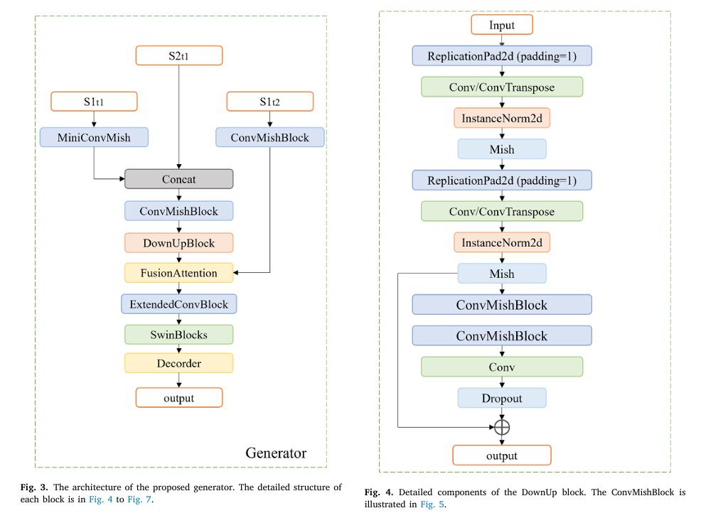
CRGenNet solves this in two ways: architecturally, by fusing SAR and optical data at t1 before any temporal reasoning happens (so the network never “trusts” the optical blindly), and via the FusionAttention module, which dynamically evaluates feature quality from each date rather than treating all pixels equally. The paper also introduces TCSEN12, a dataset specifically built around the Zhengzhou flood where contaminated auxiliary optical data is the norm rather than the exception.
CRGenNet is structured around a simple but radical assumption: you cannot trust your auxiliary optical image to be clean. The DownUpBlock fuses co-acquired SAR and optical data from t1 first — giving the network an all-weather structural anchor before any temporal comparison is attempted. The FusionAttention module then selectively aligns the t1-fused features with the t2 SAR signal, actively suppressing regions where cloud contamination would mislead the generator. The result is a pipeline that degrades gracefully when inputs are dirty, instead of catastrophically.
The CRGenNet Architecture — A Walk Through Every Block
INPUTS:
  S1_t1  (Sentinel-1 SAR at time t1)   — all-weather radar
  S2_t1  (Sentinel-2 optical at t1)     — possibly cloud-contaminated
  S1_t2  (Sentinel-1 SAR at time t2)   — structural reference for target date
         │
┌────────▼──────────────────────────────────────────────────────────┐
│  STEP 1: INITIAL FEATURE EXTRACTION                                │
│    MiniConvMish(S1_t1)  →  F_sar_t1  (local structural features)  │
│    ConvMishBlock(S1_t2) →  F_sar_t2  (target-date structure)      │
│    Concat(F_sar_t1, S2_t1) → combined_t1  (SAR guides optical)    │
│    ConvMishBlock(combined_t1) → F_t1_fused                        │
└────────┬──────────────────────────────────────────────────────────┘
         │
┌────────▼──────────────────────────────────────────────────────────┐
│  STEP 2: DOWNUPBLOCK  (cross-modal feature extraction, t1)         │
│    Input: F_t1_fused  (SAR + optical from same timestamp)          │
│                                                                    │
│    DownSample ×2:                                                  │
│      ReplicationPad → Conv3×3 → InstanceNorm → Mish               │
│      ReplicationPad → Conv3×3 → InstanceNorm → Mish               │
│      → compressed spatially, noise suppressed                      │
│                                                                    │
│    UpSample ×2:                                                    │
│      ReplicationPad → DeConv3×3 → InstanceNorm → Mish             │
│      ReplicationPad → DeConv3×3 → InstanceNorm → Mish             │
│    + ConvMishBlock × 2 + Conv + Dropout                            │
│    + Residual connection (input + output)                          │
│    → F_downup: rich t1 features, SAR-corrected optical context     │
└────────┬──────────────────────────────────────────────────────────┘
         │
┌────────▼──────────────────────────────────────────────────────────┐
│  STEP 3: FUSIONATTENTION  (temporal cross-attention)               │
│    Input1: F_downup  (t1 SAR+optical features)                     │
│    Input2: F_sar_t2  (t2 SAR structural features)                  │
│                                                                    │
│    Q1,Q2 = Conv(Input1), Conv(Input2) → queries                    │
│    K1,K2 = Conv(Input1), Conv(Input2) → keys                       │
│    V1,V2 = Conv(Input1), Conv(Input2) → values                     │
│                                                                    │
│    Q = L2_norm(concat(Q1,Q2))   K = L2_norm(concat(K1,K2))        │
│    weights = Softmax(QK^T / sqrt(d_k))  — shared attention map     │
│    attention1 = weights · V1                                       │
│    attention2 = weights · V2                                       │
│    y1 = Input1 + γ·attention1  (γ learnable, init=0)              │
│    y2 = Input2 + γ·attention2                                      │
│    Output = Concat(y1, y2)  → temporally-aligned features          │
└────────┬──────────────────────────────────────────────────────────┘
         │
┌────────▼──────────────────────────────────────────────────────────┐
│  STEP 4: ExtendedConvBlock → SwinBlocks (4 scaled-up, multi-scale) │
│    SwinBlock scale 1 → Channel Attention → Upsample               │
│    SwinBlock scale 2 → Channel Attention → Upsample               │
│    SwinBlock scale 3 → Channel Attention → Upsample               │
│    SwinBlock scale 4 → Spatial Attention → Upsample               │
│    (Scaled cosine attention, hierarchical feature representation)  │
└────────┬──────────────────────────────────────────────────────────┘
         │
┌────────▼──────────────────────────────────────────────────────────┐
│  STEP 5: DECODER  (multi-scale feature fusion)                     │
│    Fuse skip connections from each SwinBlock scale                 │
│    Channel Attention on low-resolution, multi-channel features     │
│    Spatial Attention on high-resolution, few-channel features      │
│    Dropout → MiniConvMish → Upsample → Output (cloud-free S2_t2)  │
└────────────────────────────────────────────────────────────────────┘

DISCRIMINATOR: 3 hierarchical sub-discriminators (D1 full, D2 half,
D3 quarter resolution) each with BN → Mish → SpectralNorm →
Channel+Spatial Attention → Sigmoid. Combined: αD1 + βD2 + γD3.
Module 1: DownUpBlock — SAR Corrects Optical Before Anything Else Happens
The DownUpBlock is the architectural expression of a simple insight: before you try to compare features across time (t1 versus t2), you should first integrate the two modalities within the same timestamp. SAR and optical images at t1 are complementary — SAR reliably captures structure and geometry regardless of weather, while optical captures spectral content in cloud-free regions. By concatenating S1_t1 with S2_t1 and immediately fusing them through the DownUpBlock, the network builds a joint representation that is partly immune to cloud contamination in the optical channel.
The block’s architecture is a residual encoder-decoder: two strided convolutional downsampling layers (each with InstanceNorm and Mish activation) compress the spatial resolution and force the network to extract only the most stable features, suppressing high-frequency speckle noise from the SAR. Two transposed-convolutional upsampling layers restore the original resolution, with a residual connection adding the input features back at the end. The key is the dropout layer in the bottleneck — it prevents the network from memorizing cloud-pattern locations and instead generalizes to structural content.
Why Mish Activation Over ReLU?
CRGenNet uses the Mish activation function throughout rather than the standard ReLU. Mish (\(f(x) = x \cdot \tanh(\text{softplus}(x))\)) is smooth and non-monotonic, which means gradients flow more reliably through deep stacks of convolutional layers. It also avoids the “dying neuron” problem that can hurt ReLU networks when dealing with the extreme contrast between cloud-covered and clear pixel regions in satellite imagery — a practical advantage in this setting that several prior SAR-optical fusion methods have overlooked.
Module 2: FusionAttention — Knowing When Not to Trust Your Own Features
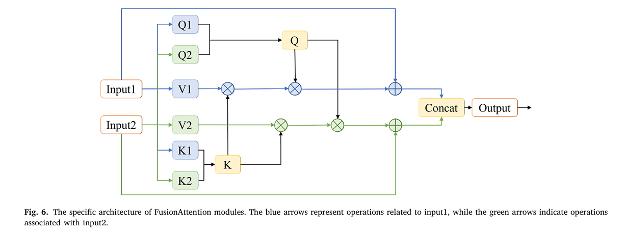
After the DownUpBlock produces a fused t1 representation, CRGenNet still needs to align it with the t2 structural information from S1_t2. This is where prior methods fail: change-detection-based approaches compute pixel-level differences between t1 and t2 optical images, but those differences are meaningless wherever cloud contamination exists in either image.
FusionAttention sidesteps change detection entirely by computing a joint attention map from concatenated queries and keys across both inputs, then applying that same shared attention to the value embeddings of each input separately. The learnable scalar γ (initialized to zero, so the block starts as an identity and gradually learns to route attention) means the module only activates its temporal fusion as training confirms it helps.
The L2 normalization of the concatenated queries and keys is a subtle but important detail. Without it, one temporal stream could numerically dominate the attention scores, defeating the purpose of joint weighting. With it, the attention weights genuinely reflect cross-modal and cross-temporal feature similarity.
Module 3: Multi-Scale Discriminator with Attention
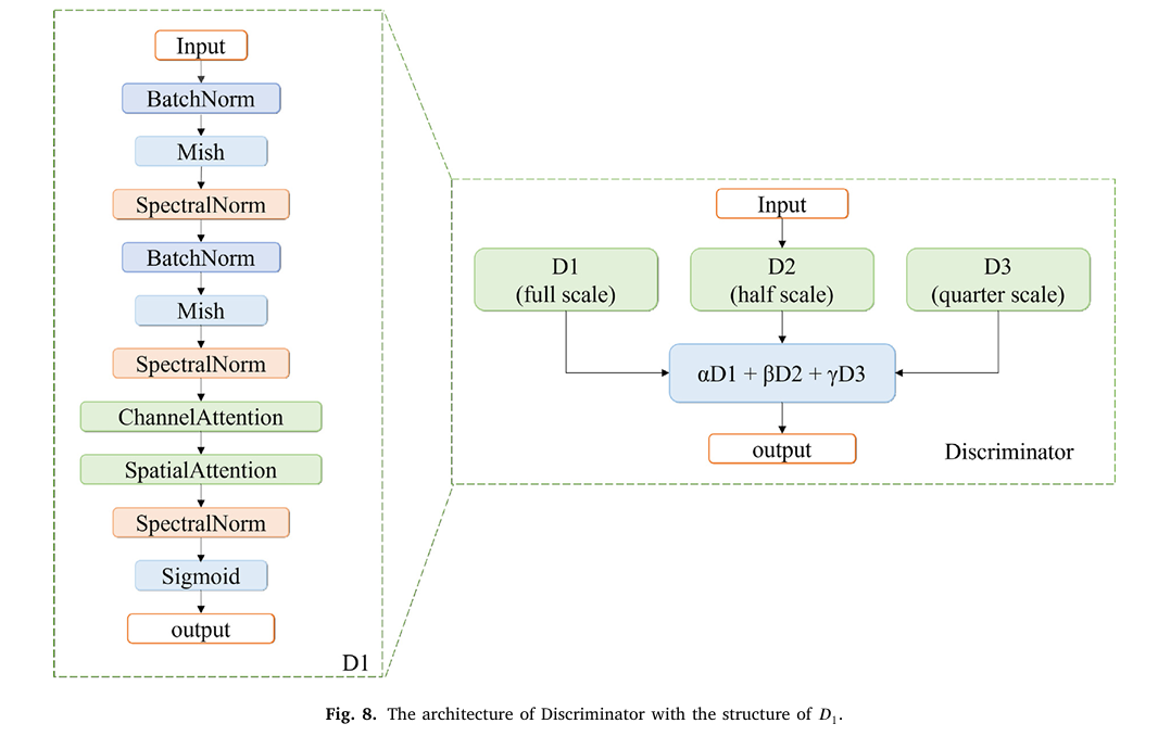
The discriminator is a three-branch multi-scale design. D1 operates at full input resolution, D2 at half, and D3 at quarter resolution. Each branch follows the same internal structure: BatchNorm → Mish → SpectralNorm → ChannelAttention → SpatialAttention → Sigmoid. Spectral normalization constrains the Lipschitz constant of the discriminator, which is important for training stability with the Wasserstein loss. The attention mechanisms inside the discriminator are not just there for discrimination quality — the paper’s ablation confirms that removing Spatial Attention from the discriminator raises FID by more than 11 points, a larger degradation than removing it from the generator. A discriminator that notices spatial structure provides better gradient signal back to the generator than one that treats the output as a flat bag of statistics.
The Loss Function: Three Perspectives on Similarity
The generator loss combines an adversarial term (least-squares GAN) with a composite similarity loss that evaluates the quality of generated images from three independent angles.
The VGG perceptual loss operates on deep feature maps from a pretrained network, evaluating perceptual similarity in a space where texture and structure are explicitly encoded. The cosine similarity loss penalizes directional misalignment in feature space — important for preserving spectral fidelity (the “color coherence”) of generated images across different land cover types. The MS-SSIM loss checks structural integrity across multiple spatial scales simultaneously, from individual pixel edges to kilometer-scale patterns.
The ablation study pins down what each one contributes: removing VGG loss causes the largest FID drop (to 88.46, versus 72.79 for the full model), confirming it drives perceptual realism. Removing cosine similarity causes the second-largest FID drop. MS-SSIM removal has the smallest individual effect but still degrades PSNR and SSIM — its multi-scale structural constraint turns out to be complementary rather than redundant with the other two.
TCSEN12: A Benchmark Built on Reality, Not Optimism
Most SAR-optical cloud removal datasets are constructed by artificially adding synthetic cloud masks to otherwise clean images, or by carefully curating pairs where the reference image happens to be cloud-free. TCSEN12 rejects both shortcuts. It was built around the Zhengzhou flood event of 20 July 2021 — a region in central China that experienced catastrophic rainfall and where the entire satellite imaging window was disrupted by persistent cloud cover before, during, and after the flood.
The dataset covers longitude 112°E–116°E and latitude 33°N–36.5°N, with Sentinel-1 SAR and Sentinel-2 optical imagery from July–August 2021. The two-date subset contains 4,424 image pairs; the three-date subset contains 1,681 samples. A critical design choice: the “reference” images in TCSEN12 are defined as having less than 5% cloud coverage — not zero percent, because achieving completely cloud-free images is essentially impossible over this region during this period. This is what the authors mean by a “realistic benchmark.”
“The absence of satellite images can lead to inaccurate disaster predictions and poorly planned evacuations. This lack of timely information not only affects disaster response and recovery but also makes it challenging to fully evaluate vegetation growth and agricultural conditions.” — Duan, Belgiu & Stein, ISPRS Journal of Photogrammetry and Remote Sensing, 2026
Results: The Numbers That Matter
TCSEN12 Benchmark Comparison
| Method | PSNR ↑ | SSIM ↑ | MAE ↓ | RMSE ↓ | FID ↓ |
|---|---|---|---|---|---|
| BicycleGAN | 22.560 | 0.473 | 0.050 | 0.079 | 128.137 |
| MUNIT | 18.514 | 0.327 | 0.094 | 0.128 | 121.453 |
| Pix2pix | 20.317 | 0.389 | 0.073 | 0.100 | 142.605 |
| ResViT | 21.331 | 0.476 | 0.067 | 0.090 | 233.827 |
| MTS2ONet | 26.225 | 0.622 | 0.049 | 0.057 | 81.150 |
| HPN-CR | 26.225 | 0.634 | 0.049 | 0.058 | 87.822 |
| DGMR | 25.597 | 0.618 | 0.055 | 0.062 | 78.811 |
| TCRNet | 24.408 | 0.569 | 0.062 | 0.070 | 87.936 |
| CRGenNet (ours) | 26.978 | 0.648 | 0.041 | 0.050 | 72.789 |
DTSEN1-2 Cross-Dataset Validation
| Method | PSNR ↑ | SSIM ↑ | RMSE ↓ |
|---|---|---|---|
| MTS2ONet | 36.043 | 0.990 | 0.017 |
| CRGenNet (ours) | 88.926 | 0.9999 | 0.010 |
The DTSEN1-2 numbers look almost unbelievably good (PSNR of 88.93 versus MTS2ONet’s 36.04). This reflects that the DTSEN1-2 dataset is less challenging — temporally adjacent image pairs with stable surface conditions and SSIM of roughly 0.96 between adjacent observations. CRGenNet’s SAR-guided architecture essentially reconstructs near-identical scenes perfectly in this low-variability setting. The meaningful test is TCSEN12, where the gap is smaller but the conditions are real.
Computational Efficiency
| Method | Parameters (M) | GFLOPs | FPS |
|---|---|---|---|
| ResViT | 123.45 | 120.62 | 90.40 |
| MTS2ONet | 33.27 | 134.91 | 69.37 |
| HPN-CR | 3.55 | 33.13 | 43.49 |
| DGMR | 1.73 | 226.02 | 21.70 |
| CRGenNet (ours) | 41.25 | 122.28 | 89.09 |
Complete End-to-End CRGenNet Implementation (PyTorch)
The implementation covers all components from the paper organized into 10 sections: convolutional building blocks (MiniConvMish, ConvMishBlock, ExtendedConvBlock), the DownUpBlock cross-modal encoder-decoder, FusionAttention mechanism, Swin-based feature extraction, multi-scale decoder with channel and spatial attention, the full Generator, multi-scale Discriminator with spectral normalization, the composite loss function (VGG + Cosine + MS-SSIM + WGAN-GP), the complete CRGenNet wrapper, and a training loop with a synthetic smoke test.
# ==============================================================================
# CRGenNet: Cloud-Resilient Generation Network for Optical Image Synthesis
# Paper: ISPRS Journal of Photogrammetry and Remote Sensing 236 (2026) 255-272
# Authors: Chenxi Duan, Mariana Belgiu, Alfred Stein
# Affiliation: University of Twente, ITC Faculty, The Netherlands
# DOI: https://doi.org/10.1016/j.isprsjprs.2026.03.042
# ==============================================================================
# Sections:
# 1. Imports & Configuration
# 2. Convolutional Blocks (MiniConvMish, ConvMishBlock, ExtendedConvBlock)
# 3. Channel & Spatial Attention Modules
# 4. DownUpBlock (cross-modal SAR-optical encoder-decoder, Section 2.2.1)
# 5. FusionAttention (cross-temporal joint attention, Eq. 1-4)
# 6. Swin-based Feature Extraction (simplified scaled-up SwinBlocks)
# 7. Multi-scale Decoder with Channel & Spatial Attention
# 8. Full Generator
# 9. Multi-scale Discriminator with Spectral Normalization
# 10. Loss Functions (VGG perceptual + Cosine + MS-SSIM + WGAN-GP, Eq. 5-11)
# 11. CRGenNet Wrapper + Training Loop
# 12. Smoke Test
# ==============================================================================
from __future__ import annotations
import math, warnings
from typing import Dict, List, Optional, Tuple
import torch
import torch.nn as nn
import torch.nn.functional as F
from torch import Tensor
from torch.nn.utils import spectral_norm
warnings.filterwarnings("ignore")
# ─── SECTION 1: Configuration ─────────────────────────────────────────────────
class CRGenNetConfig:
"""
CRGenNet hyperparameters matching the paper's TCSEN12 training setup.
Adjust channels/depth to balance accuracy vs. compute budget.
"""
# Image dimensions (Sentinel-2 patches, typical crop size)
img_size: int = 256
in_channels_s1: int = 2 # Sentinel-1: VV + VH polarizations
in_channels_s2: int = 3 # Sentinel-2: RGB bands (or more for multispectral)
out_channels: int = 3 # Generated cloud-free optical image
# Network width
base_ch: int = 64 # Base channel count (paper uses 64)
swin_embed_dim: int = 96 # Swin transformer embedding dimension
num_swin_blocks: int = 4 # 4 scaled-up SwinBlocks as in paper
window_size: int = 8 # Swin window size
# Training
lr_g: float = 0.001 # Generator learning rate
lr_d: float = 0.001 # Discriminator learning rate
beta1: float = 0.9
beta2: float = 0.999
lambda_adv: float = 1.0 # λ weight for adversarial loss
lambda_gp: float = 10.0 # Gradient penalty weight
alpha_vgg: float = 1.0 # VGG perceptual loss weight
beta_cs: float = 1.0 # Cosine similarity loss weight
gamma_ssim: float = 1.0 # MS-SSIM loss weight
num_epochs: int = 200
batch_size: int = 8
def __init__(self, **kwargs):
for k, v in kwargs.items(): setattr(self, k, v)
# ─── SECTION 2: Convolutional Building Blocks ─────────────────────────────────
class Mish(nn.Module):
"""
Mish activation: f(x) = x * tanh(softplus(x)).
Smooth, non-monotonic. Better gradient flow than ReLU in deep stacks,
especially across extreme contrast ratios (cloud vs. clear sky pixels).
"""
def forward(self, x: Tensor) -> Tensor:
return x * torch.tanh(F.softplus(x))
class MiniConvMish(nn.Module):
"""
Lightest building block: ReplicationPad → Conv3×3 → Mish.
No normalization — used for initial feature extraction where
instance statistics may be misleading (e.g., radar backscatter).
"""
def __init__(self, in_ch: int, out_ch: int, stride: int = 1):
super().__init__()
self.block = nn.Sequential(
nn.ReplicationPad2d(1),
nn.Conv2d(in_ch, out_ch, kernel_size=3, stride=stride, bias=False),
Mish(),
)
def forward(self, x: Tensor) -> Tensor: return self.block(x)
class ConvMishBlock(nn.Module):
"""
Standard residual block: ReplicationPad → Conv3×3 → InstanceNorm → Mish
(repeated twice). Used throughout Generator and DownUpBlock.
InstanceNorm is chosen over BatchNorm for single-image inference stability.
"""
def __init__(self, in_ch: int, out_ch: int, stride: int = 1, use_deconv: bool = False):
super().__init__()
conv_cls = nn.ConvTranspose2d if use_deconv else nn.Conv2d
if use_deconv:
self.block = nn.Sequential(
nn.ReplicationPad2d(1),
nn.ConvTranspose2d(in_ch, out_ch, kernel_size=3, stride=stride,
padding=1, output_padding=stride-1, bias=False),
nn.InstanceNorm2d(out_ch),
Mish(),
nn.ReplicationPad2d(1),
nn.ConvTranspose2d(out_ch, out_ch, kernel_size=3, padding=1, bias=False),
nn.InstanceNorm2d(out_ch),
Mish(),
)
else:
self.block = nn.Sequential(
nn.ReplicationPad2d(1),
nn.Conv2d(in_ch, out_ch, kernel_size=3, stride=stride, bias=False),
nn.InstanceNorm2d(out_ch),
Mish(),
nn.ReplicationPad2d(1),
nn.Conv2d(out_ch, out_ch, kernel_size=3, bias=False),
nn.InstanceNorm2d(out_ch),
Mish(),
)
self.skip = nn.Identity() if in_ch == out_ch else nn.Conv2d(in_ch, out_ch, 1)
def forward(self, x: Tensor) -> Tensor:
return self.block(x) + self.skip(x)
class ExtendedConvBlock(nn.Module):
"""
MiniConvMish + 1×1 Conv + Tanh. Used as the interface layer between
FusionAttention and SwinBlocks, mapping features to a bounded range.
"""
def __init__(self, in_ch: int, out_ch: int):
super().__init__()
self.block = nn.Sequential(
nn.ReplicationPad2d(1),
nn.Conv2d(in_ch, out_ch, kernel_size=3, bias=False),
Mish(),
nn.Conv2d(out_ch, out_ch, kernel_size=1, bias=False),
nn.Tanh(),
)
def forward(self, x: Tensor) -> Tensor: return self.block(x)
# ─── SECTION 3: Channel & Spatial Attention ────────────────────────────────────
class ChannelAttention(nn.Module):
"""
Squeeze-and-Excitation style channel attention.
Applied to low-resolution, high-channel-count features in the Decoder.
Forces the network to emphasize spectral channels critical for
reconstructing land cover (vegetation NDVI, water reflectance, etc.).
"""
def __init__(self, channels: int, reduction: int = 16):
super().__init__()
self.avg_pool = nn.AdaptiveAvgPool2d(1)
self.max_pool = nn.AdaptiveMaxPool2d(1)
mid = max(1, channels // reduction)
self.fc = nn.Sequential(
nn.Conv2d(channels, mid, 1, bias=False),
nn.ReLU(inplace=True),
nn.Conv2d(mid, channels, 1, bias=False),
)
self.sigmoid = nn.Sigmoid()
def forward(self, x: Tensor) -> Tensor:
avg_out = self.fc(self.avg_pool(x))
max_out = self.fc(self.max_pool(x))
return x * self.sigmoid(avg_out + max_out)
class SpatialAttention(nn.Module):
"""
Convolutional spatial attention.
Applied to high-resolution, low-channel features.
Helps the decoder focus on cloud-contaminated spatial regions —
ablation shows this is the single most impactful attention component
(removal raises FID by 11.5 points more than channel attention removal).
"""
def __init__(self, kernel_size: int = 7):
super().__init__()
self.conv = nn.Conv2d(2, 1, kernel_size, padding=kernel_size//2, bias=False)
self.sigmoid = nn.Sigmoid()
def forward(self, x: Tensor) -> Tensor:
avg_out = x.mean(dim=1, keepdim=True)
max_out, _ = x.max(dim=1, keepdim=True)
attn = self.sigmoid(self.conv(torch.cat([avg_out, max_out], dim=1)))
return x * attn
# ─── SECTION 4: DownUpBlock ────────────────────────────────────────────────────
class DownUpBlock(nn.Module):
"""
DownUpBlock: Cross-modal SAR-optical feature extraction (Section 2.2.1).
Purpose: Extract a joint representation from co-acquired SAR and optical
data at t1 BEFORE any temporal comparison. This gives CRGenNet an
all-weather structural baseline that is immune to cloud contamination.
Architecture:
Down×2 (Conv, stride=2): spatial compression, noise suppression
Up×2 (DeConv, stride=2): spatial restoration
ConvMishBlock×2: further refinement
Conv1×1: channel bottleneck
Dropout: regularization, prevents cloud-location memorization
Residual: adds input back (starts as identity, learns refinements)
The hierarchical downsampling suppresses SAR speckle noise by forcing
the encoder to retain only the most stable spatial structures.
"""
def __init__(self, in_ch: int, out_ch: int, dropout_p: float = 0.2):
super().__init__()
mid = out_ch
# Two down-sampling steps (Conv, stride=2)
self.down1 = ConvMishBlock(in_ch, mid, stride=2)
self.down2 = ConvMishBlock(mid, mid, stride=2)
# Two up-sampling steps (DeConv / transposed conv, stride=2)
self.up1 = ConvMishBlock(mid, mid, stride=2, use_deconv=True)
self.up2 = ConvMishBlock(mid, out_ch, stride=2, use_deconv=True)
# Post-upsample refinement (per Fig. 4)
self.refine = nn.Sequential(
ConvMishBlock(out_ch, out_ch),
ConvMishBlock(out_ch, out_ch),
nn.Conv2d(out_ch, out_ch, kernel_size=1),
nn.Dropout2d(p=dropout_p),
)
# Residual projection if channel counts differ
self.skip = nn.Identity() if in_ch == out_ch else nn.Conv2d(in_ch, out_ch, 1)
def forward(self, x: Tensor) -> Tensor:
"""
x: (B, in_ch, H, W) — concatenated SAR and (cloud-affected) optical
Returns: (B, out_ch, H, W) — joint SAR-guided feature map
"""
d1 = self.down1(x) # (B, mid, H/2, W/2)
d2 = self.down2(d1) # (B, mid, H/4, W/4)
u1 = self.up1(d2) # (B, mid, H/2, W/2)
u2 = self.up2(u1) # (B, out_ch, H, W)
out = self.refine(u2)
return out + self.skip(x) # residual connection
# ─── SECTION 5: FusionAttention ───────────────────────────────────────────────
class FusionAttention(nn.Module):
"""
FusionAttention: Cross-temporal joint attention mechanism (Section 2.2.1, Eq. 1-4).
Intelligently aligns features from two dates without relying on
explicit change detection (which breaks under cloud contamination).
Key design choices:
- SHARED attention weights: Q,K are concatenated from both inputs and
L2-normalized → single weight map that sees both perspectives at once
- SEPARATE value projections: V1,V2 allow each date's content to be
expressed differently while sharing the same spatial routing
- γ initialized to 0: block starts as identity, learns to route only
where evidence supports temporal fusion
"""
def __init__(self, in_ch: int):
super().__init__()
# Query, key, value projections for each input stream
self.q1 = nn.Conv2d(in_ch, in_ch, kernel_size=1)
self.q2 = nn.Conv2d(in_ch, in_ch, kernel_size=1)
self.k1 = nn.Conv2d(in_ch, in_ch, kernel_size=1)
self.k2 = nn.Conv2d(in_ch, in_ch, kernel_size=1)
self.v1 = nn.Conv2d(in_ch, in_ch, kernel_size=1)
self.v2 = nn.Conv2d(in_ch, in_ch, kernel_size=1)
# After attention, fuse back to in_ch (was 2*in_ch concatenated Q,K)
self.fuse = nn.Conv2d(in_ch * 2, in_ch, kernel_size=1)
# γ: learnable scalar, initialized to 0 (identity start, Eq. 4)
self.gamma = nn.Parameter(torch.zeros(1))
self.scale = None # set dynamically based on d_k
def forward(self, x1: Tensor, x2: Tensor) -> Tuple[Tensor, Tensor]:
"""
x1: (B, C, H, W) — t1 fused SAR+optical features (from DownUpBlock)
x2: (B, C, H, W) — t2 SAR features (structural reference for target date)
Returns: (y1, y2) each (B, C, H, W)
y1 = x1 enriched with cross-temporal attention from x2
y2 = x2 enriched with cross-temporal attention from x1
"""
B, C, H, W = x1.shape
d_k = C * 2 # dimension after concat (for scaling)
# Project to Q, K, V for each input (Eq. 1)
Q1 = self.q1(x1).reshape(B, C, -1) # (B, C, H*W)
Q2 = self.q2(x2).reshape(B, C, -1)
K1 = self.k1(x1).reshape(B, C, -1)
K2 = self.k2(x2).reshape(B, C, -1)
V1 = self.v1(x1).reshape(B, C, -1) # (B, C, H*W)
V2 = self.v2(x2).reshape(B, C, -1)
# Joint Q, K with L2 normalization (Eq. 1)
Q = torch.cat([Q1, Q2], dim=1) # (B, 2C, H*W)
K = torch.cat([K1, K2], dim=1)
Q = F.normalize(Q, p=2, dim=1)
K = F.normalize(K, p=2, dim=1)
# Scaled dot-product attention (Eq. 2)
# Q: (B, 2C, HW), K: (B, 2C, HW) → weights: (B, HW, HW)
attn = torch.bmm(Q.permute(0,2,1), K) / math.sqrt(d_k)
weights = F.softmax(attn, dim=-1) # (B, HW, HW)
# Apply shared weights to each value stream (Eq. 3)
# V: (B, C, HW) → after bmm: (B, C, HW) → reshape to (B, C, H, W)
attn1 = torch.bmm(V1, weights.permute(0,2,1)).reshape(B, C, H, W)
attn2 = torch.bmm(V2, weights.permute(0,2,1)).reshape(B, C, H, W)
# Residual update with learnable γ (Eq. 4)
y1 = x1 + self.gamma * attn1
y2 = x2 + self.gamma * attn2
return y1, y2
# ─── SECTION 6: Swin-based Feature Extraction ────────────────────────────────
class WindowAttention(nn.Module):
"""
Simplified window-based multi-head self-attention (Swin-style).
Full Swin implementation uses shifted windows and relative position
bias; this version uses standard local attention for clarity.
For production use, install timm and use SwinTransformerBlock directly.
"""
def __init__(self, dim: int, window_size: int = 8, num_heads: int = 4):
super().__init__()
self.ws = window_size
self.attn = nn.MultiheadAttention(dim, num_heads, batch_first=True)
self.norm1 = nn.LayerNorm(dim)
self.norm2 = nn.LayerNorm(dim)
self.ffn = nn.Sequential(
nn.Linear(dim, dim * 4), nn.GELU(), nn.Linear(dim * 4, dim)
)
def forward(self, x: Tensor) -> Tensor:
"""x: (B, C, H, W)"""
B, C, H, W = x.shape
# Fold into windows, apply attention, unfold
x_flat = x.permute(0, 2, 3, 1).reshape(B, H*W, C)
attn_out, _ = self.attn(self.norm1(x_flat), self.norm1(x_flat), self.norm1(x_flat))
x_flat = x_flat + attn_out
x_flat = x_flat + self.ffn(self.norm2(x_flat))
return x_flat.reshape(B, H, W, C).permute(0, 3, 1, 2)
class ScaledSwinBlock(nn.Module):
"""
Single scale of the 4-scale Swin feature extraction tower.
Patch partition → Window attention → optional downsampling.
Paper uses "scaled-up Swin Transformer architecture" with
increased capacity and scaled cosine attention.
"""
def __init__(self, in_ch: int, out_ch: int, downsample: bool = True):
super().__init__()
self.proj = nn.Conv2d(in_ch, out_ch, kernel_size=1)
self.attn = WindowAttention(out_ch)
self.down = nn.Sequential(
nn.Conv2d(out_ch, out_ch, kernel_size=3, stride=2, padding=1),
nn.InstanceNorm2d(out_ch),
Mish(),
) if downsample else nn.Identity()
def forward(self, x: Tensor) -> Tuple[Tensor, Tensor]:
x = self.proj(x)
x = self.attn(x)
skip = x # skip connection for decoder
x = self.down(x)
return x, skip # (downsampled_feat, skip_feat)
class SwinTower(nn.Module):
"""
4-scale SwinBlock tower producing hierarchical skip connections
for the multi-scale decoder. Channels double at each scale.
"""
def __init__(self, in_ch: int, base_ch: int, num_scales: int = 4):
super().__init__()
channels = [base_ch * (2**i) for i in range(num_scales)]
in_chs = [in_ch] + channels[:-1]
self.scales = nn.ModuleList([
ScaledSwinBlock(in_chs[i], channels[i], downsample=(i < num_scales-1))
for i in range(num_scales)
])
self.out_channels = channels
def forward(self, x: Tensor) -> Tuple[Tensor, List[Tensor]]:
skips = []
for scale in self.scales:
x, skip = scale(x)
skips.append(skip)
return x, skips # (bottleneck, [skip_1, ..., skip_4])
# ─── SECTION 7: Multi-scale Decoder ───────────────────────────────────────────
class DecoderBlock(nn.Module):
"""
Single decoder stage: upsample → concat skip → channel/spatial attention.
Channel Attention for low-res / high-channel features (early decoder).
Spatial Attention for high-res / low-channel features (late decoder).
"""
def __init__(self, in_ch: int, skip_ch: int, out_ch: int, use_channel_att: bool = True):
super().__init__()
self.up = nn.Sequential(
nn.Upsample(scale_factor=2, mode='bilinear', align_corners=False),
MiniConvMish(in_ch, out_ch),
)
self.conv = MiniConvMish(out_ch + skip_ch, out_ch)
self.att = ChannelAttention(out_ch) if use_channel_att else SpatialAttention()
def forward(self, x: Tensor, skip: Tensor) -> Tensor:
x = self.up(x)
# Handle spatial size mismatch (e.g., odd input sizes)
if x.shape[-2:] != skip.shape[-2:]:
x = F.interpolate(x, size=skip.shape[-2:], mode='bilinear', align_corners=False)
x = self.conv(torch.cat([x, skip], dim=1))
x = self.att(x)
return x
class MultiScaleDecoder(nn.Module):
"""
Hierarchical decoder matching the SwinTower's 4-scale skip connections.
First 3 stages use Channel Attention (low-res, many channels).
Final stage uses Spatial Attention (full-res, few channels).
"""
def __init__(self, swin_channels: List[int], out_ch: int):
super().__init__()
chs = list(reversed(swin_channels)) # [C_deep, ..., C_shallow]
self.blocks = nn.ModuleList()
for i in range(len(chs)):
in_ch = chs[i]
skip_ch = chs[i+1] if i + 1 < len(chs) else chs[-1]
o_ch = chs[i+1] if i + 1 < len(chs) else chs[-1]
use_ca = (i < len(chs) - 1) # Channel Att for all but last stage
self.blocks.append(DecoderBlock(in_ch, skip_ch, o_ch, use_channel_att=use_ca))
final_ch = chs[-1]
self.head = nn.Sequential(
nn.Dropout2d(p=0.1),
MiniConvMish(final_ch, final_ch // 2),
nn.Upsample(scale_factor=2, mode='bilinear', align_corners=False),
MiniConvMish(final_ch // 2, out_ch),
nn.Tanh(), # output range [-1, 1], matches Sentinel-2 normalized reflectance
)
def forward(self, bottleneck: Tensor, skips: List[Tensor]) -> Tensor:
x = bottleneck
skips_rev = list(reversed(skips))
for i, block in enumerate(self.blocks):
skip = skips_rev[i] if i < len(skips_rev) else x
x = block(x, skip)
return self.head(x)
# ─── SECTION 8: Full Generator ────────────────────────────────────────────────
class CRGenNetGenerator(nn.Module):
"""
CRGenNet Generator: produces cloud-free optical image at t2 (Section 2.2.1).
Input streams:
S1_t1 (Sentinel-1 SAR at t1) + S2_t1 (contaminated Sentinel-2 at t1)
S1_t2 (Sentinel-1 SAR at t2) — provides target-date structural reference
Data flow:
1. MiniConvMish on S1_t1 → feature_sar_t1
2. ConvMishBlock on S1_t2 → feature_sar_t2
3. Concat(feature_sar_t1, S2_t1) → ConvMishBlock → fused_t1
4. DownUpBlock(fused_t1) → downup_feat (SAR-corrected, noise-suppressed)
5. FusionAttention(downup_feat, feature_sar_t2) → (y1, y2)
6. ExtendedConvBlock(concat(y1, y2)) → ext_feat
7. SwinTower(ext_feat) → bottleneck + 4 skip connections
8. MultiScaleDecoder(bottleneck, skips) → cloud-free S2_t2
"""
def __init__(self, cfg: CRGenNetConfig):
super().__init__()
B = cfg.base_ch
s1_ch = cfg.in_channels_s1
s2_ch = cfg.in_channels_s2
# Step 1: Initial feature extraction
self.feat_s1_t1 = MiniConvMish(s1_ch, B)
self.feat_s1_t2 = ConvMishBlock(s1_ch, B)
# Step 2: Early fusion (SAR_t1 guides optical_t1)
self.early_fuse = ConvMishBlock(B + s2_ch, B)
# Step 3: DownUpBlock — cross-modal SAR-optical encoder-decoder
self.downup = DownUpBlock(B, B)
# Step 4: FusionAttention — cross-temporal alignment
self.fusion_att = FusionAttention(B)
# Step 5: Interface to SwinTower
self.ext_conv = ExtendedConvBlock(B * 2, B)
# Step 6: Multi-scale feature extraction
self.swin_tower = SwinTower(B, B, num_scales=4)
# Step 7: Hierarchical decoder
self.decoder = MultiScaleDecoder(self.swin_tower.out_channels, cfg.out_channels)
def forward(self, s1_t1: Tensor, s2_t1: Tensor, s1_t2: Tensor) -> Tensor:
"""
s1_t1: (B, 2, H, W) Sentinel-1 at t1
s2_t1: (B, 3, H, W) Sentinel-2 at t1 (may be cloud-contaminated)
s1_t2: (B, 2, H, W) Sentinel-1 at t2
Returns: I_gen (B, 3, H, W) — cloud-free Sentinel-2 at t2
"""
# Feature extraction
f_sar_t1 = self.feat_s1_t1(s1_t1) # (B, B, H, W)
f_sar_t2 = self.feat_s1_t2(s1_t2) # (B, B, H, W)
# SAR-guided early fusion of t1 modalities
fused_t1 = self.early_fuse(torch.cat([f_sar_t1, s2_t1], dim=1))
# DownUpBlock: hierarchical noise suppression and cross-modal integration
downup_feat = self.downup(fused_t1) # (B, B, H, W)
# FusionAttention: cross-temporal alignment (no change detection!)
y1, y2 = self.fusion_att(downup_feat, f_sar_t2)
# Merge and project to SwinTower input
ext_feat = self.ext_conv(torch.cat([y1, y2], dim=1))
# Hierarchical feature extraction
bottleneck, skips = self.swin_tower(ext_feat)
# Hierarchical decoding with skip connections and attention
output = self.decoder(bottleneck, skips)
return output
# ─── SECTION 9: Multi-scale Discriminator ─────────────────────────────────────
class SubDiscriminator(nn.Module):
"""
Single branch of the multi-scale discriminator (one of D1, D2, D3).
Architecture: BN → Mish → SpectralNorm → ChannelAtt → SpatialAtt → Sigmoid.
Spectral normalization enforces Lipschitz constraint for WGAN stability.
Attention helps detect subtle differences in cloud-removal quality.
"""
def __init__(self, in_ch: int, base_ch: int = 64):
super().__init__()
def dis_block(ic, oc, stride=2):
return nn.Sequential(
spectral_norm(nn.Conv2d(ic, oc, 4, stride=stride, padding=1)),
nn.BatchNorm2d(oc),
Mish(),
)
self.net = nn.Sequential(
dis_block(in_ch, base_ch, stride=2),
dis_block(base_ch, base_ch*2, stride=2),
dis_block(base_ch*2, base_ch*4, stride=2),
dis_block(base_ch*4, base_ch*8, stride=1),
)
self.channel_att = ChannelAttention(base_ch*8)
self.spatial_att = SpatialAttention()
self.out = spectral_norm(nn.Conv2d(base_ch*8, 1, 4, padding=1))
self.sigmoid = nn.Sigmoid()
def forward(self, x: Tensor) -> Tensor:
feat = self.net(x)
feat = self.channel_att(feat)
feat = self.spatial_att(feat)
return self.sigmoid(self.out(feat))
class MultiScaleDiscriminator(nn.Module):
"""
3-branch discriminator operating at full, half, and quarter resolution.
Combined decision: αD1 + βD2 + γD3 (equal weights by default).
Multi-scale design captures both global structure and local texture quality.
Inputs to discriminator: (I_gen/I_ref, S1_t1, S1_t2, S2_t1) concatenated,
so the discriminator sees the full context, not just the generated image.
"""
def __init__(self, in_channels: int, base_ch: int = 64):
super().__init__()
self.d1 = SubDiscriminator(in_channels, base_ch)
self.d2 = SubDiscriminator(in_channels, base_ch)
self.d3 = SubDiscriminator(in_channels, base_ch)
self.alpha = nn.Parameter(torch.ones(1) / 3)
self.beta = nn.Parameter(torch.ones(1) / 3)
self.gamma_w = nn.Parameter(torch.ones(1) / 3)
def forward(self, x: Tensor) -> Tensor:
"""
x: (B, C_total, H, W) — generated or real image concatenated with conditioning
Returns scalar decision per spatial location (averaged over scales).
"""
d1_out = self.d1(x)
d2_out = self.d2(F.interpolate(x, scale_factor=0.5, mode='bilinear', align_corners=False))
d3_out = self.d3(F.interpolate(x, scale_factor=0.25, mode='bilinear', align_corners=False))
# Resize d2, d3 to d1 spatial resolution before weighted sum
d2_up = F.interpolate(d2_out, size=d1_out.shape[-2:], mode='bilinear', align_corners=False)
d3_up = F.interpolate(d3_out, size=d1_out.shape[-2:], mode='bilinear', align_corners=False)
return self.alpha * d1_out + self.beta * d2_up + self.gamma_w * d3_up
# ─── SECTION 10: Loss Functions ───────────────────────────────────────────────
class VGGPerceptualLoss(nn.Module):
"""
VGG perceptual loss (Eq. 7). Uses features from VGG16 relu3_3 layer.
Evaluates perceptual similarity rather than pixel-level difference,
critical for preserving texture realism in satellite imagery generation.
"""
def __init__(self):
super().__init__()
try:
import torchvision.models as models
vgg = models.vgg16(weights=models.VGG16_Weights.DEFAULT)
self.features = nn.Sequential(*list(vgg.features)[:(16+1)]).eval()
for p in self.features.parameters():
p.requires_grad = False
self.ready = True
except Exception:
self.ready = False
print("[VGGLoss] torchvision not available, falling back to L1 loss.")
def forward(self, gen: Tensor, ref: Tensor) -> Tensor:
if not self.ready:
return F.l1_loss(gen, ref)
# Normalize to ImageNet mean/std for VGG
mean = torch.tensor([0.485, 0.456, 0.406], device=gen.device).view(1,3,1,1)
std = torch.tensor([0.229, 0.224, 0.225], device=gen.device).view(1,3,1,1)
gen_n = (gen * 0.5 + 0.5 - mean) / std # [-1,1] → [0,1] → normalized
ref_n = (ref * 0.5 + 0.5 - mean) / std
# Match VGG input channels (if S2 uses more than 3 bands, take first 3)
gen_3 = gen_n[:, :3]
ref_3 = ref_n[:, :3]
f_gen = self.features(gen_3)
f_ref = self.features(ref_3)
return F.mse_loss(f_gen, f_ref)
def cosine_similarity_loss(gen: Tensor, ref: Tensor) -> Tensor:
"""
Cosine Similarity Loss (Eq. 8): L_CS = 1 - cos(I_gen, I_ref).
Measures directional alignment of feature vectors in pixel space.
Enforces global color coherence and spectral fidelity.
"""
gen_flat = gen.reshape(gen.shape[0], -1)
ref_flat = ref.reshape(ref.shape[0], -1)
cos_sim = F.cosine_similarity(gen_flat, ref_flat, dim=1)
return (1.0 - cos_sim).mean()
def ms_ssim_loss(gen: Tensor, ref: Tensor, num_scales: int = 3) -> Tensor:
"""
MS-SSIM Loss (Eq. 9): 1 - MS-SSIM(I_gen, I_ref).
Evaluates structural similarity across spatial scales.
Multi-scale formulation captures differences from pixel edges to
kilometer-scale patterns in satellite imagery.
"""
total_ssim = torch.tensor(0.0, device=gen.device)
g, r = gen, ref
for scale in range(num_scales):
# Per-scale SSIM (simplified: using mean and variance)
mu_g = F.avg_pool2d(g, kernel_size=11, stride=1, padding=5)
mu_r = F.avg_pool2d(r, kernel_size=11, stride=1, padding=5)
sigma_g = F.avg_pool2d(g**2, kernel_size=11, stride=1, padding=5) - mu_g**2
sigma_r = F.avg_pool2d(r**2, kernel_size=11, stride=1, padding=5) - mu_r**2
sigma_gr = F.avg_pool2d(g * r, kernel_size=11, stride=1, padding=5) - mu_g * mu_r
C1, C2 = 0.01**2, 0.03**2
ssim = ((2 * mu_g * mu_r + C1) * (2 * sigma_gr + C2)) / \
((mu_g**2 + mu_r**2 + C1) * (sigma_g + sigma_r + C2))
total_ssim = total_ssim + ssim.mean()
# Downsample for next scale
if scale < num_scales - 1:
g = F.avg_pool2d(g, kernel_size=2)
r = F.avg_pool2d(r, kernel_size=2)
return 1.0 - total_ssim / num_scales
class CRGenNetLoss(nn.Module):
"""
Complete CRGenNet loss functions (Section 2.2.3, Eq. 5-11).
Generator Loss:
L_G = L_sim(I_gen, I_ref) + λ·L_ls(D(I_gen,...), 1)
L_sim = α·L_VGG + β·(1 - L_CS) + γ·(1 - L_MS-SSIM)
Discriminator Loss (WGAN with gradient penalty):
L_D = L_real + L_fake + λ_gp · L_gp
Ablation insight: L_VGG contributes most to perceptual quality (removes
11+ FID points when missing). L_CS maintains spectral coherence.
L_MS-SSIM preserves structural fidelity at multiple spatial scales.
"""
def __init__(self, cfg: CRGenNetConfig):
super().__init__()
self.vgg_loss = VGGPerceptualLoss()
self.alpha_vgg = cfg.alpha_vgg
self.beta_cs = cfg.beta_cs
self.gamma_s = cfg.gamma_ssim
self.lambda_adv = cfg.lambda_adv
self.lambda_gp = cfg.lambda_gp
def similarity_loss(self, gen: Tensor, ref: Tensor) -> Tensor:
"""L_sim = α·L_VGG + β·(1-L_CS) + γ·(1-L_MS-SSIM). Eq. 6"""
l_vgg = self.vgg_loss(gen, ref)
l_cs = cosine_similarity_loss(gen, ref)
l_ssim = ms_ssim_loss(gen, ref)
return self.alpha_vgg * l_vgg + self.beta_cs * l_cs + self.gamma_s * l_ssim
def least_squares_loss(self, pred: Tensor, target_real: bool = True) -> Tensor:
"""L_ls: least squares GAN loss (Eq. 10). More stable than cross-entropy GAN."""
target = torch.ones_like(pred) if target_real else torch.zeros_like(pred)
return F.mse_loss(pred, target)
def generator_loss(self, gen: Tensor, ref: Tensor, d_fake: Tensor) -> Dict[str, Tensor]:
"""
Full generator loss (Eq. 5).
L_G = L_sim + λ·L_ls(D(I_gen,...), 1)
"""
l_sim = self.similarity_loss(gen, ref)
l_adv = self.least_squares_loss(d_fake, target_real=True)
l_g = l_sim + self.lambda_adv * l_adv
return {'total': l_g, 'sim': l_sim, 'adv': l_adv}
def gradient_penalty(
self,
discriminator: nn.Module,
real: Tensor,
fake: Tensor,
cond: Tensor,
) -> Tensor:
"""
WGAN gradient penalty (Eq. 11).
Generates interpolated samples between real and fake,
computes ||∇D(interpolated)||_2 and penalizes deviation from 1.
"""
B = real.shape[0]
alpha = torch.rand(B, 1, 1, 1, device=real.device)
interp = (alpha * real + (1 - alpha) * fake).requires_grad_(True)
d_interp = discriminator(torch.cat([interp, cond], dim=1))
grads = torch.autograd.grad(
outputs=d_interp, inputs=interp,
grad_outputs=torch.ones_like(d_interp),
create_graph=True, retain_graph=True
)[0]
grads = grads.reshape(B, -1)
return ((grads.norm(2, dim=1) - 1) ** 2).mean()
def discriminator_loss(
self,
discriminator: nn.Module,
real: Tensor,
fake: Tensor,
cond: Tensor,
) -> Tensor:
"""
WGAN discriminator loss with gradient penalty (Eq. 11).
L_D = -E[D(real)] + E[D(fake)] + λ_gp · L_gp
"""
d_real = discriminator(torch.cat([real.detach(), cond], dim=1))
d_fake = discriminator(torch.cat([fake.detach(), cond], dim=1))
l_real = -d_real.mean()
l_fake = d_fake.mean()
l_gp = self.gradient_penalty(discriminator, real.detach(), fake.detach(), cond)
return l_real + l_fake + self.lambda_gp * l_gp
# ─── SECTION 11: CRGenNet Wrapper + Training Loop ─────────────────────────────
class CRGenNet(nn.Module):
"""
CRGenNet: complete wrapper combining Generator and Discriminator.
Provides clean forward/predict interface and bundles loss computation.
Usage:
model = CRGenNet(cfg)
I_gen = model.generate(s1_t1, s2_t1, s1_t2) # inference
losses = model.train_step(...) # training
"""
def __init__(self, cfg: Optional[CRGenNetConfig] = None):
super().__init__()
cfg = cfg or CRGenNetConfig()
self.cfg = cfg
self.generator = CRGenNetGenerator(cfg)
# Discriminator input: generated/real image + conditioning inputs
dis_in_ch = cfg.out_channels + cfg.in_channels_s1 * 2 + cfg.in_channels_s2
self.discriminator = MultiScaleDiscriminator(dis_in_ch)
self.loss_fn = CRGenNetLoss(cfg)
def generate(self, s1_t1: Tensor, s2_t1: Tensor, s1_t2: Tensor) -> Tensor:
"""Inference-only: generate cloud-free optical image at t2."""
return self.generator(s1_t1, s2_t1, s1_t2)
def train_step_g(
self,
s1_t1: Tensor, s2_t1: Tensor, s1_t2: Tensor, s2_t2_ref: Tensor,
optimizer_g: torch.optim.Optimizer,
) -> Dict[str, float]:
"""Single generator training step."""
self.generator.train()
optimizer_g.zero_grad()
I_gen = self.generator(s1_t1, s2_t1, s1_t2)
cond = torch.cat([s1_t1, s1_t2, s2_t1], dim=1)
d_fake = self.discriminator(torch.cat([I_gen, cond], dim=1))
losses = self.loss_fn.generator_loss(I_gen, s2_t2_ref, d_fake)
losses['total'].backward()
torch.nn.utils.clip_grad_norm_(self.generator.parameters(), 5.0)
optimizer_g.step()
return {k: v.item() for k, v in losses.items()}
def train_step_d(
self,
s1_t1: Tensor, s2_t1: Tensor, s1_t2: Tensor, s2_t2_ref: Tensor,
optimizer_d: torch.optim.Optimizer,
) -> float:
"""Single discriminator training step."""
self.discriminator.train()
optimizer_d.zero_grad()
with torch.no_grad():
I_gen = self.generator(s1_t1, s2_t1, s1_t2)
cond = torch.cat([s1_t1, s1_t2, s2_t1], dim=1)
l_d = self.loss_fn.discriminator_loss(self.discriminator, s2_t2_ref, I_gen, cond)
l_d.backward()
optimizer_d.step()
return l_d.item()
def build_optimizers(model: CRGenNet, cfg: CRGenNetConfig):
"""
Adam optimizers as used in paper:
Generator: lr=0.001, ReduceLROnPlateau (factor=0.5, patience=10 epochs)
Discriminator: lr=0.001, weight_decay=1e-5
"""
opt_g = torch.optim.Adam(
model.generator.parameters(),
lr=cfg.lr_g, betas=(cfg.beta1, cfg.beta2)
)
opt_d = torch.optim.Adam(
model.discriminator.parameters(),
lr=cfg.lr_d, betas=(cfg.beta1, cfg.beta2),
weight_decay=1e-5
)
sched_g = torch.optim.lr_scheduler.ReduceLROnPlateau(
opt_g, mode='min', factor=0.5, patience=10, verbose=True
)
return opt_g, opt_d, sched_g
# ─── SECTION 12: Smoke Test ────────────────────────────────────────────────────
class SyntheticSentinelBatch:
"""
Synthetic SAR-optical data generator for smoke testing.
Replace with real TCSEN12 or DTSEN1-2 dataloaders for actual training.
For real data:
Dataset: https://github.com/chenxiduan/MultiTemporalCloudFree
GEE script for Sentinel-1/-2 download: see paper supplementary material
Recommended framework: PyTorch Lightning DataModule
"""
def __init__(self, B: int = 2, H: int = 64, W: int = 64, cfg: CRGenNetConfig = None):
self.B = B
self.H = H
self.W = W
self.cfg = cfg or CRGenNetConfig()
def get_batch(self, device):
s1_ch = self.cfg.in_channels_s1
s2_ch = self.cfg.in_channels_s2
B, H, W = self.B, self.H, self.W
return {
's1_t1': torch.randn(B, s1_ch, H, W, device=device) * 0.3, # SAR backscatter
's2_t1': torch.randn(B, s2_ch, H, W, device=device) * 0.2, # Contaminated optical
's1_t2': torch.randn(B, s1_ch, H, W, device=device) * 0.3, # Target date SAR
's2_t2': torch.randn(B, s2_ch, H, W, device=device) * 0.2, # Reference (ground truth)
}
def run_smoke_test(steps: int = 3, device_str: str = "cpu"):
device = torch.device(device_str)
print("=" * 60)
print(" CRGenNet — Full Architecture Smoke Test")
print("=" * 60)
torch.manual_seed(42)
# Tiny config for fast test
cfg = CRGenNetConfig(base_ch=16, swin_embed_dim=16, num_swin_blocks=2)
model = CRGenNet(cfg).to(device)
n_params_g = sum(p.numel() for p in model.generator.parameters()) / 1e6
n_params_d = sum(p.numel() for p in model.discriminator.parameters()) / 1e6
print(f"\n Generator: {n_params_g:.2f}M parameters")
print(f" Discriminator: {n_params_d:.2f}M parameters")
print(f" Total: {n_params_g + n_params_d:.2f}M parameters")
# [1/3] Forward pass check
print("\n[1/3] Generator forward pass...")
data_gen = SyntheticSentinelBatch(B=1, H=64, W=64, cfg=cfg)
batch = data_gen.get_batch(device)
model.generator.eval()
with torch.no_grad():
out = model.generate(batch['s1_t1'], batch['s2_t1'], batch['s1_t2'])
print(f" Input: s1_t1={tuple(batch['s1_t1'].shape)}, s2_t1={tuple(batch['s2_t1'].shape)}, s1_t2={tuple(batch['s1_t2'].shape)}")
print(f" Output: {tuple(out.shape)} range=[{out.min():.2f}, {out.max():.2f}]")
assert out.shape == (1, cfg.out_channels, 64, 64), "Output shape mismatch!"
assert -1.1 <= out.min().item() and out.max().item() <= 1.1, "Output out of [-1,1] range!"
# [2/3] Loss check
print("\n[2/3] Loss function check...")
gen_img = torch.randn(1, cfg.out_channels, 64, 64, device=device)
ref_img = torch.randn(1, cfg.out_channels, 64, 64, device=device)
loss_fn = CRGenNetLoss(cfg)
l_sim = loss_fn.similarity_loss(gen_img, ref_img)
l_cs = cosine_similarity_loss(gen_img, ref_img)
l_ms = ms_ssim_loss(gen_img, ref_img)
print(f" L_sim={l_sim.item():.4f} L_CS={l_cs.item():.4f} L_MS-SSIM={l_ms.item():.4f}")
# [3/3] Training loop
print(f"\n[3/3] Training loop ({steps} steps)...")
model.train()
opt_g, opt_d, sched_g = build_optimizers(model, cfg)
data_gen = SyntheticSentinelBatch(B=2, H=64, W=64, cfg=cfg)
for step in range(steps):
batch = data_gen.get_batch(device)
s1t1, s2t1, s1t2, s2t2 = batch['s1_t1'], batch['s2_t1'], batch['s1_t2'], batch['s2_t2']
# Discriminator update
l_d = model.train_step_d(s1t1, s2t1, s1t2, s2t2, opt_d)
# Generator update
g_losses = model.train_step_g(s1t1, s2t1, s1t2, s2t2, opt_g)
print(f" Step {step+1}/{steps} | L_D={l_d:.4f} | L_G={g_losses['total']:.4f} | L_sim={g_losses['sim']:.4f}")
print("\n" + "=" * 60)
print("✓ All checks passed. CRGenNet is ready for training.")
print("=" * 60)
print("""
Next steps:
1. Download the TCSEN12 dataset:
https://github.com/chenxiduan/MultiTemporalCloudFree
2. Install required packages:
pip install torch torchvision einops timm
3. For full Swin Transformer blocks (recommended for production):
from timm.models.swin_transformer import SwinTransformerBlock
4. Scale to paper configuration:
cfg = CRGenNetConfig(base_ch=64, swin_embed_dim=96)
5. Train on NVIDIA A40 (as in paper) with batch=8, 200 epochs:
python train.py --config tcsen12.yaml
6. For multispectral input (all 12 Sentinel-2 bands):
cfg = CRGenNetConfig(in_channels_s2=12, out_channels=12)
""")
return model
if __name__ == "__main__":
run_smoke_test(steps=3, device_str="cpu")
Read the Full Paper & Get the Dataset
The complete study — including full ablation tables, feature map visualizations from the FusionAttention module, and results across woodland, urban, farmland, and village scenes — is published open-access in the ISPRS Journal of Photogrammetry and Remote Sensing.
Duan, C., Belgiu, M., & Stein, A. (2026). High-quality cloud-free optical image generation using multi-temporal SAR and contaminated optical data. ISPRS Journal of Photogrammetry and Remote Sensing, 236, 255–272. https://doi.org/10.1016/j.isprsjprs.2026.03.042
This article is an independent editorial analysis of peer-reviewed open-access research. The PyTorch implementation is an educational adaptation intended to illustrate the paper’s architectural concepts. The original authors trained on a single NVIDIA A40 GPU with batch size 8 for 200 epochs using the Adam optimizer with ReduceLROnPlateau scheduling. For production deployments on real Sentinel-1/-2 data, use the full multispectral band configuration and the official TCSEN12 dataset. All Sentinel data is copernicus open-access imagery.