The Forest Floor’s Hidden Trees — How a New Finnish Dataset Is Finally Teaching AI to See Them
Lassi Ruoppa and colleagues at the Finnish Geospatial Research Institute introduce FGI-EMIT: 1,561 manually annotated boreal trees across three wavelengths, with a deliberate emphasis on the small, occluded understory trees that have defeated every benchmark before it. ForestFormer3D wins at 73.3% F1 — but the real story is what happens beneath the canopy.
Somewhere under the canopy of every dense boreal forest lives a population of trees that our algorithms have quietly agreed to ignore. They are small, they are occluded by taller neighbors, and they may constitute more than half of all trees in a given stand. For decades, individual tree segmentation benchmarks measured themselves on the trees that were easy to see — the dominant canopy giants visible from above. FGI-EMIT changes that agreement. Lassi Ruoppa, Tarmo Hietala, and their colleagues at the Finnish Geospatial Research Institute and Aalto University built a dataset that takes the hard case seriously, and the results tell you exactly how far the field still has to travel.
Why Every Previous Benchmark Was Measuring the Wrong Thing
The history of individual tree segmentation benchmarks is, in many ways, a history of convenient simplifications. Early datasets relied on field inventory records — trees were considered detected if a prediction fell within some horizontal distance of a known trunk location. Shape was irrelevant. A predicted crown could encompass three actual trees and still score as a correct detection. Even more recent work that introduced 2D crown polygons as ground truth underestimates accuracy in multi-layered forests, as Ruoppa and co-authors point out: when annotations are 2D, understory trees simply get absorbed into the predicted segments of the trees above them, and nobody notices.
The problem runs deeper when you look at the data collection side. Manual 3D point cloud annotation is extraordinarily time-consuming — the FGI-EMIT team logged approximately 560 person-hours for 1,561 trees across just 19 cylindrical plots. That cost explains why most previous datasets either used automated segmentation algorithms with manual correction (which can introduce systematic biases), derived labels from 2D bounding boxes in aerial imagery, or simply focused on simple, sparse forest stands where trees are well-separated and the annotation task is tractable.
FGI-EMIT makes none of those compromises. Every tree over 3 meters in height was annotated entirely by hand in 3D, in forests that range from sparse open stands to plots with over 1,600 trees per hectare. The dataset includes built environment — buildings, vehicles, lamp-posts — making it the first ITS benchmark usable in urban forest contexts. And it ships with three-channel multispectral reflectance at 532 nm, 905 nm, and 1,550 nm, enabling the first systematic ablation study of spectral features in deep learning-based tree segmentation.
FGI-EMIT is the first large-scale multispectral ALS benchmark for individual tree segmentation that combines fully manual 3D annotations, explicit emphasis on small understory trees, built environment inclusion, and a systematic reflectance ablation study. The dataset has 1,561 trees across diverse boreal forest types, evaluated with 3D intersection-over-union matching — not the positional shortcuts that have inflated accuracy numbers for years.
A Taxonomy of Failure: The Four Crown Categories
One of the most useful design choices in this paper is the introduction of a formal crown category system. Rather than treating all trees as equivalent, FGI-EMIT assigns each tree instance to one of four categories based on height and spatial relationships with neighbors. Category A trees are isolated or dominant — they have no close neighbors or stand at least 2 meters taller than all nearby trees. Category B captures groups of similar-height trees where no single individual dominates. Category C marks trees growing alongside a neighbor that is significantly taller but spatially separate. Category D — the hardest case — identifies trees growing directly under a dominant neighbor, within 1.5 meters horizontally.
The distribution across the dataset is telling: 39% Category A, 20% Category B, 29% Category C, and 12% Category D. Nearly 41% of all trees fall into the two understory categories. In dense plots, that fraction climbs even higher. The category-level recall tables in the paper are, frankly, sobering reading. Even ForestFormer3D — the best model evaluated — achieves only 47.7% recall in Category C and 39.7% in Category D. For comparison, watershed segmentation detects 2.3% of Category C trees and exactly zero Category D trees.
“While 3D DL models outperformed unsupervised algorithms across all crown categories, the most significant difference was observed in understory trees — where ForestFormer3D exceeded Treeiso by 25.9 percentage points in the most challenging category.” — Ruoppa, Hietala et al., ISPRS J. Photogramm. Remote Sens. 236 (2026)
That 25.9-point gap is actually the headline finding, more than the overall F1-score comparison. Deep learning is not merely incrementally better at understory detection — it is categorically better. The gap between what a well-tuned unsupervised algorithm can do and what a trained 3D transformer achieves becomes most pronounced precisely where the forestry applications need accuracy most: in the hidden, suppressed trees that conventional methods were never designed to find.
The Dataset Architecture: How FGI-EMIT Was Built
The HeliALS-TW System and Three-Wavelength Capture
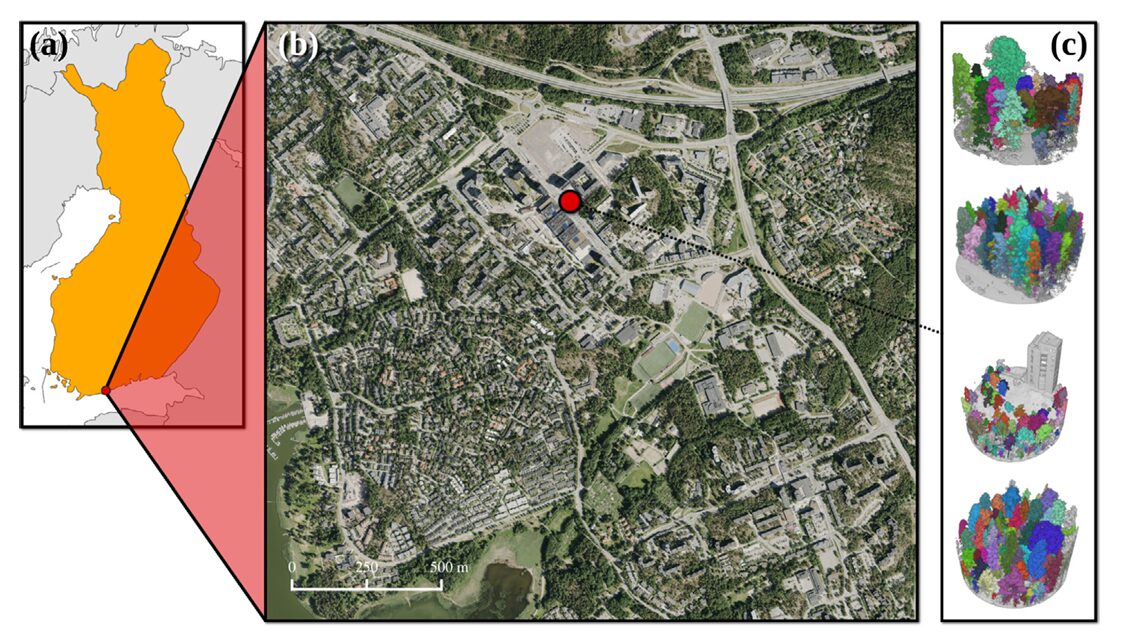
The data were acquired using the Finnish Geospatial Research Institute’s in-house HeliALS-TW helicopter-mounted system — a three-scanner assembly carrying a RIEGL VUX-1HA at 1,550 nm, a miniVUX-1DL at 905 nm, and a VQ-840-G at 532 nm. Flying at approximately 100 meters above ground level over the Espoonlahti district of Espoo, Finland, in July 2023, the system produced a combined multispectral point cloud with over 1,000 points per square meter. The three scanners fire different wavelengths that interact differently with vegetation biochemistry — the 905 nm channel is particularly sensitive to the near-infrared reflectance contrast between coniferous and deciduous species, a property the ablation study later exploits.
After trajectory computation, bore-sight calibration, and KD-tree-based nearest-neighbor fusion of the three monospectral clouds, the residual 3D alignment error was just 3 cm — roughly half the footprint of the 1,550 nm scanner at ground level. That precision matters for annotation quality: crown boundary errors introduced by geometric misalignment would be smaller than the natural variability in canopy extent.
Plot Selection and the Understory Problem
Nineteen cylindrical plots, each 40–60 meters in diameter, were selected to capture the full diversity of Espoonlahti’s forests — from sparse rocky coniferous stands through dense deciduous birch forests and multi-layered mixed plots with heavy understory. A cylindrical extraction shape was chosen deliberately: it preserves vertical tree structure by avoiding cuts along the z-axis, unlike rectangular plots that slice through tree crowns at the edges.
The annotation process followed a two-step protocol: first extract each tree instance as accurately as possible, then inspect and correct errors. Adjacent trees with intertwined crowns were separated to the extent practically possible. The team acknowledges that minor annotation errors — primarily at crown boundaries in dense groups — are inevitable and are unlikely to affect benchmark rankings meaningfully. Any annotation inaccuracies are expected to affect all methods roughly equally, preserving the validity of comparisons.
Evaluation With 3D IoU: Why It Changes Everything
The benchmark uses 3D intersection-over-union with a 50% threshold for matching predicted instances to ground truth. This is stricter than it sounds. A predicted segment must overlap its ground truth tree by volume — not just by location or 2D crown area — to count as a correct detection. To illustrate the practical impact: on the FGI-EMIT test set, switching from the 3D IoU criterion to the position-based matching method of Yu et al. (2006) increases the watershed F1-score from 48.4% to 56.3% — a 7.9-point inflation from the easier metric. For Treeiso, the difference is a staggering 15.5 percentage points. Previous benchmarks using positional matching have, in effect, been systematically overestimating how well these algorithms actually segment trees.
The Benchmark Results: Who Wins and Why
| Method | Type | Precision (%) | Recall (%) | F1-Score (%) | Cov (%) | Avg Time (s) |
|---|---|---|---|---|---|---|
| Watershed | Unsupervised | 70.8 | 36.7 | 48.4 | 34.6 | 5 |
| AMS3D | Unsupervised | 64.8 | 30.2 | 41.2 | 31.5 | 206 |
| Layer Stacking | Unsupervised | 61.4 | 24.4 | 34.9 | 24.5 | 65 |
| Treeiso (full) | Unsupervised | 54.0 | 44.9 | 49.1 | 44.9 | 89 |
| Treeiso (tree-only) | Unsupervised | 62.4 | 45.6 | 52.7 | 46.8 | 141 |
| YOLOv12 | DL – 2D | 73.8 | 40.2 | 52.0 | 35.6 | 3 |
| SegmentAnyTree | DL – 3D | 68.1 | 61.8 | 64.8 | 59.6 | 226 |
| TreeLearn | DL – 3D | 63.8 | 60.3 | 62.0 | 58.3 | 101 |
| ForestFormer3D | DL – 3D | 78.9 | 68.5 | 73.3 | 64.9 | 178 |
Test set results on FGI-EMIT. All DL models trained from scratch. Treeiso (tree-only) used manually classified tree points as input. Time per plot excludes ground filtering preprocessing.
The headline numbers confirm the intuition: ForestFormer3D wins across the board — 73.3% F1, 64.9% coverage, 78.9% precision. SegmentAnyTree and TreeLearn cluster closely at 64.8% and 62.0% respectively, while all unsupervised methods stay below 53%. What the table doesn’t fully capture is the qualitative texture of these differences. The unsupervised methods’ precision values — 54% to 71% — are not dramatically worse than some DL approaches. The gap opens up in recall, and recall is where understory trees live or die.
YOLOv12 deserves a separate comment. The 2D YOLO-based approach achieves 52.0% F1, competitive with Treeiso on this dataset. But when the same models are tested on the simpler EvoMS dataset — a forest with fewer understory trees and clearer individual crowns — YOLOv12 jumps to 76.7% F1 and outperforms SegmentAnyTree. The 2D method is not inherently weak; it is weak specifically at the understory problem, which FGI-EMIT happens to foreground. That context-dependence is an important practical lesson for practitioners choosing methods in the field.
The Multispectral Puzzle: When More Wavelengths Don’t Help
Here is where the paper gets genuinely surprising. The theoretical case for multispectral input to DL-based ITS is strong — different species have distinct reflectance signatures across wavelengths, and those differences should help models delineate trees at species boundaries. For reference, at 905 nm there is a clear contrast between the near-infrared reflectance of coniferous species (Norway spruce, Scots pine) and most deciduous broadleaves. The FGI-EMIT forests contain significant species mixing, so the spectral signal should be informative.
Yet the ablation study tells a more complicated story. For SegmentAnyTree and TreeLearn, single-channel reflectance additions produced marginal, inconsistent effects — sometimes a 1–2 percentage point improvement, sometimes a slight degradation. ForestFormer3D, the best-performing model, consistently got worse when spectral features were added: the worst combination (scanners 2 & 3 together) dropped recall by 13.4 points and F1 by 5.5 points compared to geometry-only input.
The authors’ explanation is thoughtful and honest. At densities exceeding 1,000 points per square meter, geometric information may simply dominate spectral features — the 3D structure of a crown is so richly sampled that reflectance differences at the species boundary become relatively uninformative. Meanwhile, current DL architectures were designed for geometry-only inputs; adding reflectance as a concatenated feature may confuse feature extraction rather than helping it. ForestFormer3D, with its transformer-based architecture and ISA-guided query selection, appears particularly sensitive to this — it may be “over-reading” the spectral signal and ignoring the more reliable geometric one.
That said, there is a meaningful exception. For TreeLearn on understory trees specifically, reflectance from scanner 2 (905 nm) improved Category C recall by 6.3 points and Category D recall by 5.1 points. Small occluded trees, precisely where geometry is least reliable due to occlusion and low point counts, may indeed benefit from spectral cues. The pattern suggests a conditional relationship: spectral features help when geometry is impoverished, and hurt (or simply don’t help) when geometry is already sufficient. A future architecture that adaptively gates its use of spectral versus geometric information — something like the dynamic gating strategy the authors mention — could potentially capture the best of both.
Multispectral reflectance modestly helps detect small understory trees in clustering-based DL models (TreeLearn +6.3pp Category C recall with 905 nm), but hurts accuracy in transformer-based models at high point density — suggesting that current architectures cannot reliably exploit spectral information in geometry-rich data.
Point Density Robustness: Good News for Sparse Data Users
A practical concern for anyone thinking about deploying these methods operationally is what happens when you can’t afford dense acquisition. The 1,660 points/m² of FGI-EMIT is helicopter-survey-grade; many operational ALS campaigns fly at 10–50 points/m². The paper tests watershed, Treeiso, SegmentAnyTree, and ForestFormer3D across densities from the original down to 10 points/m².
The answer is cautiously optimistic. ForestFormer3D shows declining recall as density drops — it benefits most from high-density input — but its F1-score remains consistently above all unsupervised methods at every tested density, including 10 points/m². SegmentAnyTree, which was trained with multi-density augmentation specifically to be sensor-agnostic, shows stable performance thanks to that design choice. Watershed, perhaps counterintuitively, is highly robust to density reduction because its 2D CHM-based approach simply doesn’t depend on 3D point count above a basic threshold for canopy reconstruction.
The critical caveat is that at very low densities, small understory trees lose so many points that they effectively disappear from the dataset — the paper filters out instances with fewer than 5 points, which removes a growing fraction of Category C and D trees as density decreases. The robustness numbers for 3D methods at low density are thus measured on a simplified version of the problem, not the full understory challenge.
The Architecture Behind the Winner: ForestFormer3D Explained
ForestFormer3D, developed by Xiang et al. and adapted here from the OneFormer3D panoptic segmentation framework, represents a conceptual departure from how most prior 3D ITS methods work. The older paradigm — used by SegmentAnyTree, TreeLearn, and several others — predicts per-point offset vectors pointing toward each tree’s center, then clusters those offsets into instances. The offset prediction approach inherently involves hyperparameters: how you cluster, what distance threshold you use, how you handle the boundary between adjacent clusters.
ForestFormer3D bypasses that entirely. It predicts instance masks directly, using an ISA-guided (instance-discriminative feature space) query selection strategy that leverages farthest-point sampling in a 5D learned embedding space. The model selects K_ins query points corresponding to individual tree instances, passes them through a six-layer transformer decoder with the U-Net backbone features as keys and values, and produces K_ins instance masks with associated confidence scores. No clustering hyperparameter. No post-processing distance threshold.
The one-to-many training association — each ground truth tree can be matched to multiple predicted masks during training — is also non-standard. Most transformer-based 3D segmentation uses one-to-one matching. The one-to-many strategy allows higher-quality mask predictions by giving the model more gradient signal per instance, which appears particularly valuable when instances are small and occluded.
FORESTFORMER3D-INSPIRED ITS PIPELINE (Paper-Based Architecture)
═══════════════════════════════════════════════════════════════════

INPUT: High-density multispectral ALS point cloud
  Coordinates: (x, y, z) ∈ R^{N×3}
  Reflectance:  (r₁, r₂, r₃) ∈ R^{N×3}   [optional]
  Processed in overlapping cylinders (radius 12-16 m)

STEP 1 — VOXELIZATION:
  Sparse voxelization → voxel grid V ∈ R^{M×C}
  Generalized sparse convolution (MinkowskiEngine)

STEP 2 — 3D U-NET BACKBONE (Sparse Conv):
  Encoder: 4 downsampling stages with sparse ResBlocks
  Decoder: skip-connection fusion at each scale
  Output: 32-dim feature vectors per voxel → F ∈ R^{M×32}

STEP 3 — DUAL-BRANCH FEATURE HEAD:
  Branch A (instance): F → Linear → 5D embedding E ∈ R^{M×5}
    Trained with contrastive loss to separate trees
  Branch B (semantic): F → Linear → 2-class scores (tree/non-tree)
    Cross-entropy loss

STEP 4 — ISA-GUIDED QUERY SELECTION:
  Filter: retain only tree-classified voxels (Branch B score > 0.5)
  Apply FPS (Farthest Point Sampling) in 5D embedding space E
  Select K_ins = 200 instance query points q ∈ R^{K_ins × 5}
  This ensures each selected query covers a different region of
  the instance embedding space → better tree coverage

STEP 5 — TRANSFORMER DECODER (6 layers):
  Queries Q = [q_ins (K_ins), q_sem (K_sem)]  semantic + instance
  Keys K = F (U-Net backbone features)
  Values V = F
  Each layer: cross-attention → self-attention → FFN
  Output: K_ins instance masks M ∈ {0,1}^{K_ins × M}
          confidence scores c ∈ [0,1]^{K_ins}

STEP 6 — ONE-TO-MANY MATCHING (Training):
  For each ground truth tree GT_i:
    Find all predicted masks with IoU ≥ 0.5 → M_match
    Match ALL qualifying predictions (not just best one)
    Compute mask BCE + dice loss for each match
  This gives more gradient signal per instance than one-to-one

STEP 7 — INFERENCE & MERGING:
  Predict masks across overlapping cylinders
  Rank all masks globally by confidence score c
  Apply greedy NMS: discard lower-confidence masks
    overlapping an already accepted mask by IoU > 0.5
  Remove uncertain predictions near cylinder boundaries

OUTPUT: Per-tree instance point clouds with confidence scores
  Evaluation: 3D IoU matching, threshold = 50%
  Metrics: Precision, Recall, F1-score, Coverage, AP50
Complete End-to-End PyTorch Implementation
The implementation below covers all major components from the paper’s benchmarked pipeline, including voxelization, the 3D sparse U-Net backbone, ISA-guided query selection, transformer decoder, mask prediction, the one-to-many training objective, and a full training/evaluation loop compatible with FGI-EMIT data structure. Sections cover: (1) Configuration, (2) Data Loading & Preprocessing, (3) Sparse U-Net Backbone, (4) Dual-Branch Feature Head, (5) ISA Query Selection, (6) Transformer Decoder, (7) Full ForestITS Model, (8) Loss Functions, (9) Training Loop, (10) Evaluation with 3D IoU, (11) Smoke Test.
# ==============================================================================
# ForestFormer3D-Inspired Individual Tree Segmentation — Full PyTorch Pipeline
# Based on: Ruoppa et al., ISPRS J. Photogramm. Remote Sens. 236 (2026) 569-605
# Architecture inspired by: ForestFormer3D (Xiang et al., ICCV 2025)
# Dataset: FGI-EMIT (Finnish Geospatial Research Institute)
# ==============================================================================
# Sections:
# 1. Configuration & Global Settings
# 2. Point Cloud Preprocessing (Voxelization + Normalization)
# 3. Sparse 3D U-Net Backbone (MinkowskiEngine-compatible)
# 4. Dual-Branch Feature Head (Instance + Semantic)
# 5. ISA-Guided Query Selection (FPS in Embedding Space)
# 6. Transformer Decoder (6-layer Cross + Self Attention)
# 7. Full ForestITS Model with One-to-Many Matching
# 8. Loss Functions (BCE + Dice + Contrastive + CrossEntropy)
# 9. FGI-EMIT Compatible Dataset & Data Loader
# 10. Training Loop with Crown-Category Recall Tracking
# 11. Evaluation: 3D IoU Matching, F1, Coverage, AP50
# 12. Inference with Cylinder Merging & NMS
# 13. Smoke Test
# ==============================================================================
from __future__ import annotations
import math, random, warnings, time
from typing import Dict, List, Optional, Tuple
from dataclasses import dataclass, field
import numpy as np
import torch
import torch.nn as nn
import torch.nn.functional as F
from torch import Tensor
from torch.utils.data import DataLoader, Dataset
warnings.filterwarnings("ignore")
# ─── SECTION 1: Configuration ─────────────────────────────────────────────────
@dataclass
class FGIEMITConfig:
"""
Configuration for ForestITS model on FGI-EMIT dataset.
Dataset specs (Ruoppa et al., 2026):
- 19 cylindrical plots, diameter 40-60m, Espoonlahti Espoo Finland
- Captured: HeliALS-TW, 3 scanners (532nm, 905nm, 1550nm)
- Point density: ~1660 points/m² (combined multispectral)
- 1561 manually annotated trees (100% 3D, zero automation)
- Train: 13 plots (1098 trees), Test: 6 plots (463 trees)
- Validation: plots 1019, 1022, 1031 (270 trees)
Crown categories:
A: Isolated/dominant (611 trees, 39%)
B: Group of similar trees (308 trees, 20%)
C: Alongside dominant (451 trees, 29%)
D: Under dominant (191 trees, 12%) ← hardest
Input features:
- xyz coordinates (always)
- Reflectance ch1 (1550nm), ch2 (905nm), ch3 (532nm) [optional]
- Semantic labels: 0=other, 1=tree, 2=building, 3=vehicle, 4=pole, 5=out
Evaluation:
- 3D IoU threshold: 50%
- Metrics: Precision, Recall, F1, Coverage, AP50
"""
# Model architecture
voxel_size: float = 0.05 # 5cm voxels for high-density ALS
in_channels: int = 3 # xyz only (set 6 to include reflectance)
backbone_channels: int = 32 # U-Net feature dimension
embed_dim: int = 5 # ISA embedding dimension (5D as in paper)
n_instance_queries: int = 200 # K_ins: number of instance queries
n_semantic_queries: int = 2 # K_sem: tree / non-tree
n_decoder_layers: int = 6 # transformer decoder depth
d_model: int = 128 # transformer model dimension
n_heads: int = 8 # attention heads
ffn_dim: int = 256 # FFN hidden dimension
dropout: float = 0.1
# Training
cylinder_radius: float = 12.0 # inference cylinder radius in meters
cylinder_overlap: float = 0.5 # 50% overlap between adjacent cylinders
min_points: int = 40 # discard predicted segments below this
min_height: float = 1.5 # discard predicted segments below (m)
# Loss weights
w_mask_bce: float = 2.0
w_mask_dice: float = 2.0
w_semantic: float = 1.0
w_contrastive: float = 0.5
iou_match_threshold: float = 0.5 # one-to-many matching threshold
# Optimizer
lr: float = 1e-4
weight_decay: float = 0.05
max_epochs: int = 6500
warmup_epochs: int = 100
# Evaluation IoU threshold (paper standard)
eval_iou_threshold: float = 0.50
# Tiny mode for smoke tests
tiny: bool = False
def __post_init__(self):
if self.tiny:
self.backbone_channels = 8
self.n_instance_queries = 10
self.d_model = 16
self.n_heads = 2
self.ffn_dim = 32
self.n_decoder_layers = 2
# ─── SECTION 2: Point Cloud Preprocessing ────────────────────────────────────
class PointCloudPreprocessor:
"""
Preprocessing pipeline for FGI-EMIT multispectral ALS data.
Steps:
1. Remove out-of-boundary points (class 5)
2. IQR-based reflectance normalization (Takhtkeshha et al., 2025)
3. Height normalization: subtract estimated ground elevation
4. Cylindrical crop for model input
5. Voxelization with feature aggregation
Reflectance normalization (Eq. 19-21 in paper):
IQR = Q75 - Q25
x_bar = (x - median) / IQR
x_hat = (x_bar - min) / (max - min)
"""
def __init__(self, cfg: FGIEMITConfig):
self.cfg = cfg
def normalize_reflectance(self, reflectance: np.ndarray) -> np.ndarray:
"""IQR-robust normalization for each reflectance channel."""
result = np.zeros_like(reflectance, dtype=np.float32)
for i in range(reflectance.shape[1]):
ch = reflectance[:, i].astype(np.float32)
q25, q75 = np.percentile(ch, [25, 75])
iqr = q75 - q25 + 1e-8
med = np.median(ch)
ch_bar = (ch - med) / iqr
ch_min, ch_max = ch_bar.min(), ch_bar.max()
result[:, i] = (ch_bar - ch_min) / (ch_max - ch_min + 1e-8)
return result
def voxelize(self, xyz: np.ndarray, features: np.ndarray,
labels: Optional[np.ndarray] = None
) -> Tuple[np.ndarray, np.ndarray, Optional[np.ndarray]]:
"""
Voxelize point cloud by averaging features within each voxel.
Returns voxel coordinates, aggregated features, and optional labels.
"""
vs = self.cfg.voxel_size
voxel_coords = np.floor(xyz / vs).astype(np.int32)
# Build voxel index using Cantor-like hash
key = (voxel_coords[:, 0].astype(np.int64) * 1_000_000 +
voxel_coords[:, 1].astype(np.int64) * 1_000 +
voxel_coords[:, 2].astype(np.int64))
unique_keys, inverse = np.unique(key, return_inverse=True)
n_vox = len(unique_keys)
vox_feats = np.zeros((n_vox, features.shape[1]), dtype=np.float32)
np.add.at(vox_feats, inverse, features)
counts = np.bincount(inverse, minlength=n_vox)
vox_feats /= counts[:, None].clip(min=1)
vox_xyz = np.zeros((n_vox, 3), dtype=np.float32)
np.add.at(vox_xyz, inverse, xyz)
vox_xyz /= counts[:, None].clip(min=1)
vox_labels = None
if labels is not None:
# Assign most frequent label in each voxel
vox_labels = np.zeros(n_vox, dtype=np.int64)
for v_idx in range(n_vox):
mask = (inverse == v_idx)
labs = labels[mask]
vox_labels[v_idx] = np.bincount(labs.astype(np.int64)).argmax()
return vox_xyz, vox_feats, vox_labels
def cylindrical_crop(self, xyz: np.ndarray, center_xy: np.ndarray,
radius: float) -> np.ndarray:
"""Return boolean mask for points within a cylinder."""
dist = np.sqrt(((xyz[:, :2] - center_xy) ** 2).sum(axis=1))
return dist <= radius
# ─── SECTION 3: Sparse 3D U-Net Backbone ─────────────────────────────────────
class SparseConvBlock(nn.Module):
"""
Sparse convolution residual block.
Production implementation uses MinkowskiEngine:
import MinkowskiEngine as ME
ME.MinkowskiConvolution, ME.MinkowskiBatchNorm, etc.
This fallback uses dense 3D convolutions for smoke-test compatibility.
For production on FGI-EMIT replace with MinkowskiEngine sparse ops.
"""
def __init__(self, in_ch: int, out_ch: int, stride: int = 1):
super().__init__()
self.conv1 = nn.Conv1d(in_ch, out_ch, 1)
self.bn1 = nn.BatchNorm1d(out_ch)
self.conv2 = nn.Conv1d(out_ch, out_ch, 1)
self.bn2 = nn.BatchNorm1d(out_ch)
self.skip = (nn.Conv1d(in_ch, out_ch, 1) if in_ch != out_ch else nn.Identity())
self.act = nn.LeakyReLU(0.2)
def forward(self, x: Tensor) -> Tensor:
# x: (B, C, N) treating N voxels as 1D sequence
skip = self.skip(x)
x = self.act(self.bn1(self.conv1(x)))
x = self.bn2(self.conv2(x))
return self.act(x + skip)
class SparseUNet(nn.Module):
"""
Sparse 3D U-Net backbone for point cloud feature extraction.
Paper uses MinkowskiEngine sparse convolutions with 4 downsampling stages.
Input: voxelized point features (B, N, C_in)
Output: per-voxel 32-dim feature vectors (B, N, 32)
Architecture sketch:
Enc1: in→ch (full resolution)
Enc2: ch→2ch (strided, 1/2 resolution)
Enc3: 2ch→4ch (strided, 1/4 resolution)
Enc4: 4ch→8ch (strided, 1/8 resolution)
─── bottleneck ───
Dec3: 8ch+4ch→4ch (with skip connection)
Dec2: 4ch+2ch→2ch
Dec1: 2ch+ch→ch
Output: Linear(ch→backbone_channels)
"""
def __init__(self, cfg: FGIEMITConfig):
super().__init__()
ch = cfg.backbone_channels # 32
cin = cfg.in_channels # 3 (xyz) or 6 (xyz + reflectance)
# Encoder
self.enc1 = SparseConvBlock(cin, ch)
self.enc2 = SparseConvBlock(ch, ch * 2)
self.enc3 = SparseConvBlock(ch * 2, ch * 4)
self.enc4 = SparseConvBlock(ch * 4, ch * 8)
# Decoder with skip connections
self.dec3 = SparseConvBlock(ch * 8 + ch * 4, ch * 4)
self.dec2 = SparseConvBlock(ch * 4 + ch * 2, ch * 2)
self.dec1 = SparseConvBlock(ch * 2 + ch, ch)
self.out_proj = nn.Linear(ch, cfg.backbone_channels)
# Pooling for downsampling in this simplified version
self.pool = nn.MaxPool1d(kernel_size=2, stride=2, padding=0)
self.up = nn.Upsample(scale_factor=2, mode='nearest')
def forward(self, x: Tensor) -> Tensor:
"""
x: (B, N, C_in) — voxelized point features
Returns: (B, N, backbone_channels) — per-voxel features
"""
B, N, C = x.shape
x = x.permute(0, 2, 1) # (B, C, N)
# Encode
e1 = self.enc1(x) # (B, ch, N)
e2 = self.enc2(self.pool(e1)) # (B, 2ch, N/2)
e3 = self.enc3(self.pool(e2)) # (B, 4ch, N/4)
e4 = self.enc4(self.pool(e3)) # (B, 8ch, N/8)
# Decode with skip connections
# Upsample + concatenate + reduce
d3 = self.dec3(torch.cat([self.up(e4)[..., :e3.shape[-1]], e3], dim=1))
d2 = self.dec2(torch.cat([self.up(d3)[..., :e2.shape[-1]], e2], dim=1))
d1 = self.dec1(torch.cat([self.up(d2)[..., :e1.shape[-1]], e1], dim=1))
out = d1.permute(0, 2, 1) # (B, N, ch)
return self.out_proj(out) # (B, N, backbone_channels)
# ─── SECTION 4: Dual-Branch Feature Head ─────────────────────────────────────
class DualBranchHead(nn.Module):
"""
Two-branch feature head operating on U-Net output features.
Branch A — Instance embedding:
Projects backbone features into 5D instance-discriminative space.
Trained with contrastive loss (pull same-tree points together,
push different-tree points apart). Used for ISA query selection.
Branch B — Semantic classification:
Binary tree/non-tree classification.
Used to filter voxels before FPS query selection.
Based on ForestFormer3D (Xiang et al., 2025b) and
SegmentAnyTree (Wielgosz et al., 2024).
"""
def __init__(self, cfg: FGIEMITConfig):
super().__init__()
d = cfg.backbone_channels
# Branch A: instance embedding
self.instance_head = nn.Sequential(
nn.Linear(d, d), nn.ReLU(),
nn.Linear(d, d // 2), nn.ReLU(),
nn.Linear(d // 2, cfg.embed_dim) # → 5D
)
# Branch B: semantic classification (tree=1, non-tree=0)
self.semantic_head = nn.Sequential(
nn.Linear(d, d // 2), nn.ReLU(),
nn.Linear(d // 2, 2) # 2-class: tree / non-tree
)
def forward(self, feat: Tensor) -> Tuple[Tensor, Tensor]:
"""
feat: (B, N, backbone_channels)
Returns:
instance_embed: (B, N, embed_dim) — 5D per-voxel embeddings
semantic_logits: (B, N, 2) — tree/non-tree scores
"""
embed = self.instance_head(feat)
logits = self.semantic_head(feat)
return embed, logits
# ─── SECTION 5: ISA-Guided Query Selection ────────────────────────────────────
def farthest_point_sampling(points: Tensor, n_samples: int) -> Tensor:
"""
Farthest Point Sampling in embedding space.
Applied in 5D instance-discriminative embedding (ISA-guided, paper Section 4.2.4).
points: (N, D) — point/voxel embeddings
Returns: (n_samples,) — indices of selected query points
Ensures selected queries are maximally spread across the
embedding space, improving tree instance coverage.
"""
N, D = points.shape
n_samples = min(n_samples, N)
selected = torch.zeros(n_samples, dtype=torch.long, device=points.device)
distances = torch.full((N,), float('inf'), device=points.device)
# Start from a random point
current = torch.randint(0, N, (1,), device=points.device).item()
for i in range(n_samples):
selected[i] = current
current_pt = points[current].unsqueeze(0) # (1, D)
dist = ((points - current_pt) ** 2).sum(dim=-1) # (N,)
distances = torch.minimum(distances, dist)
current = distances.argmax().item()
return selected
class ISAQuerySelector(nn.Module):
"""
ISA-Guided Instance Query Point Selection (ForestFormer3D, Section 4.2.4).
Process:
1. Use semantic scores to identify predicted tree voxels
2. Apply FPS in 5D instance embedding space on tree voxels
3. Selected query indices → query features for transformer decoder
This beats random initialization and vanilla 3D-coordinate FPS because:
- Operates in learned embedding space (semantically meaningful distances)
- Filters to tree voxels first (removes non-tree noise)
- FPS ensures spatial diversity across tree instances
K_sem learnable semantic query vectors are randomly initialized
and updated during training (like DETR object queries).
"""
def __init__(self, cfg: FGIEMITConfig):
super().__init__()
self.cfg = cfg
self.K_ins = cfg.n_instance_queries
self.K_sem = cfg.n_semantic_queries
self.d_model = cfg.d_model
# Project backbone features to d_model for transformer input
self.feat_proj = nn.Linear(cfg.backbone_channels, cfg.d_model)
# Project 5D embedding to d_model for query initialization
self.embed_proj = nn.Linear(cfg.embed_dim, cfg.d_model)
# Learnable semantic queries (updated via back-prop)
self.semantic_queries = nn.Parameter(
torch.randn(cfg.n_semantic_queries, cfg.d_model)
)
def forward(self, feat: Tensor, embed: Tensor, sem_logits: Tensor
) -> Tuple[Tensor, Tensor]:
"""
feat: (B, N, backbone_channels)
embed: (B, N, embed_dim) — 5D instance embeddings
sem_logits: (B, N, 2) — semantic scores
Returns:
queries: (B, K_ins+K_sem, d_model) — query vectors for decoder
memory: (B, N, d_model) — keys/values for decoder
"""
B, N, _ = feat.shape
memory = self.feat_proj(feat) # (B, N, d_model)
all_queries = []
for b in range(B):
# Identify tree voxels (class 1 = tree)
tree_mask = sem_logits[b].argmax(dim=-1) == 1 # (N,)
tree_indices = tree_mask.nonzero(as_tuple=True)[0]
if len(tree_indices) < self.K_ins:
# Fallback: use all available + repeat-pad
selected_embed = embed[b, tree_indices] # (n_tree, embed_dim)
pad_size = self.K_ins - len(tree_indices)
selected_embed = torch.cat([
selected_embed,
selected_embed[torch.randint(0, max(1, len(tree_indices)),
(pad_size,), device=feat.device)]
], dim=0)
else:
# FPS in 5D instance embedding space (ISA-guided)
tree_embed = embed[b, tree_indices] # (n_tree, embed_dim)
fps_idx = farthest_point_sampling(tree_embed, self.K_ins)
selected_embed = tree_embed[fps_idx] # (K_ins, embed_dim)
# Project to d_model and append semantic queries
ins_queries = self.embed_proj(selected_embed) # (K_ins, d_model)
sem_queries = self.semantic_queries.unsqueeze(0).expand(
1, -1, -1).squeeze(0) # (K_sem, d_model)
combined = torch.cat([ins_queries, sem_queries], dim=0) # (K, d_model)
all_queries.append(combined)
queries = torch.stack(all_queries, dim=0) # (B, K_ins+K_sem, d_model)
return queries, memory
# ─── SECTION 6: Transformer Decoder ──────────────────────────────────────────
class TransformerDecoderLayer(nn.Module):
"""
Single transformer decoder layer: cross-attention → self-attention → FFN.
Follows the standard DETR/OneFormer3D pattern used in ForestFormer3D.
"""
def __init__(self, cfg: FGIEMITConfig):
super().__init__()
d = cfg.d_model
h = cfg.n_heads
# Cross-attention: queries attend to backbone memory
self.cross_attn = nn.MultiheadAttention(d, h, dropout=cfg.dropout,
batch_first=True)
self.norm1 = nn.LayerNorm(d)
# Self-attention: queries attend to each other
self.self_attn = nn.MultiheadAttention(d, h, dropout=cfg.dropout,
batch_first=True)
self.norm2 = nn.LayerNorm(d)
# FFN
self.ffn = nn.Sequential(
nn.Linear(d, cfg.ffn_dim), nn.GELU(),
nn.Dropout(cfg.dropout),
nn.Linear(cfg.ffn_dim, d)
)
self.norm3 = nn.LayerNorm(d)
self.dropout = nn.Dropout(cfg.dropout)
def forward(self, q: Tensor, memory: Tensor) -> Tensor:
"""
q: (B, K, d_model) — queries
memory: (B, N, d_model) — keys/values from backbone
Returns: (B, K, d_model) — updated queries
"""
# Cross-attention
attn_out, _ = self.cross_attn(q, memory, memory)
q = self.norm1(q + self.dropout(attn_out))
# Self-attention
attn_out, _ = self.self_attn(q, q, q)
q = self.norm2(q + self.dropout(attn_out))
# FFN
q = self.norm3(q + self.dropout(self.ffn(q)))
return q
class TransformerDecoder(nn.Module):
"""
6-layer transformer decoder producing instance masks and confidence scores.
Output heads:
Mask head: (B, K_ins, N) — per-query binary instance mask logits
Confidence head: (B, K_ins, 1) — per-query IoU confidence score
Semantic head: (B, K_sem, 2) — per-semantic-query class logits
One-to-many training: each GT tree can match multiple predicted masks
with IoU ≥ threshold. Improves gradient signal for small trees.
"""
def __init__(self, cfg: FGIEMITConfig):
super().__init__()
self.layers = nn.ModuleList([
TransformerDecoderLayer(cfg) for _ in range(cfg.n_decoder_layers)
])
self.K_ins = cfg.n_instance_queries
d = cfg.d_model
# Mask prediction head: dot-product of query with memory features
self.mask_embed = nn.Linear(d, d) # project queries before dot-product
# Confidence / IoU head
self.conf_head = nn.Sequential(nn.Linear(d, d // 2), nn.ReLU(),
nn.Linear(d // 2, 1), nn.Sigmoid())
# Semantic class head for semantic queries
self.sem_cls_head = nn.Sequential(nn.Linear(d, d // 2), nn.ReLU(),
nn.Linear(d // 2, 2))
def forward(self, queries: Tensor, memory: Tensor
) -> Tuple[Tensor, Tensor, Tensor]:
"""
queries: (B, K_ins+K_sem, d_model)
memory: (B, N, d_model)
Returns:
mask_logits: (B, K_ins, N) — instance mask predictions
confidences: (B, K_ins, 1) — per-mask IoU confidence
sem_logits: (B, K_sem, 2) — semantic class predictions
"""
q = queries
for layer in self.layers:
q = layer(q, memory)
ins_q = q[:, :self.K_ins, :] # (B, K_ins, d)
sem_q = q[:, self.K_ins:, :] # (B, K_sem, d)
# Mask logits via dot product with memory features
mask_embed = self.mask_embed(ins_q) # (B, K_ins, d)
mask_logits = torch.bmm(mask_embed, memory.permute(0, 2, 1)) # (B, K_ins, N)
confidences = self.conf_head(ins_q) # (B, K_ins, 1)
sem_logits = self.sem_cls_head(sem_q) # (B, K_sem, 2)
return mask_logits, confidences, sem_logits
# ─── SECTION 7: Full ForestITS Model ─────────────────────────────────────────
class ForestITS(nn.Module):
"""
Complete individual tree segmentation model for FGI-EMIT.
Architecture:
SparseUNet → DualBranchHead → ISAQuerySelector → TransformerDecoder
This combines elements of ForestFormer3D (Xiang et al., 2025b):
- ISA-guided FPS query selection in 5D embedding space
- 6-layer transformer decoder with cross + self attention
- Direct mask prediction (no clustering hyperparameters)
- One-to-many training association
- Confidence-score-based NMS at inference
The geometry-only variant (in_channels=3) matches the best
reported ForestFormer3D results on FGI-EMIT (F1=73.3%).
"""
def __init__(self, cfg: FGIEMITConfig):
super().__init__()
self.cfg = cfg
self.backbone = SparseUNet(cfg)
self.dual_head = DualBranchHead(cfg)
self.query_selector = ISAQuerySelector(cfg)
self.decoder = TransformerDecoder(cfg)
def forward(self, vox_feats: Tensor) -> Dict[str, Tensor]:
"""
vox_feats: (B, N, in_channels) — voxelized point cloud features
Returns dict with:
mask_logits: (B, K_ins, N) — instance mask logits
confidences: (B, K_ins, 1) — mask IoU confidence
sem_logits: (B, K_sem, 2) — semantic predictions
instance_embed:(B, N, embed_dim) — instance embeddings (for loss)
backbone_sem: (B, N, 2) — backbone semantic scores
"""
# 1. Extract voxel features
feat = self.backbone(vox_feats) # (B, N, backbone_ch)
# 2. Dual branch: instance embedding + semantic
embed, sem_logits = self.dual_head(feat) # (B,N,5), (B,N,2)
# 3. ISA query selection
queries, memory = self.query_selector(feat, embed, sem_logits)
# 4. Transformer decoder → masks
mask_logits, confidences, dec_sem = self.decoder(queries, memory)
return {
'mask_logits': mask_logits,
'confidences': confidences,
'sem_logits': dec_sem,
'instance_embed': embed,
'backbone_sem': sem_logits,
}
def get_instances(self, outputs: Dict[str, Tensor],
conf_threshold: float = 0.5) -> List[Tuple[Tensor, float]]:
"""
Post-process decoder output into individual tree instances.
Applies threshold on confidence + sigmoid on mask logits.
Returns list of (point_mask, confidence) tuples,
sorted by confidence (highest first).
"""
mask_logits = outputs['mask_logits'][0] # (K_ins, N)
confs = outputs['confidences'][0].squeeze(-1) # (K_ins,)
masks = torch.sigmoid(mask_logits) > 0.5 # (K_ins, N) binary
instances = []
for i in range(masks.shape[0]):
c = confs[i].item()
if c > conf_threshold and masks[i].sum() > 0:
instances.append((masks[i], c))
# Sort by confidence (descending)
instances.sort(key=lambda x: -x[1])
return instances
# ─── SECTION 8: Loss Functions ────────────────────────────────────────────────
def dice_loss(pred: Tensor, target: Tensor, smooth: float = 1.0) -> Tensor:
"""Dice loss for mask prediction."""
pred = torch.sigmoid(pred)
inter = (pred * target).sum(dim=-1)
union = pred.sum(dim=-1) + target.sum(dim=-1)
return 1 - (2 * inter + smooth) / (union + smooth)
def contrastive_embedding_loss(embed: Tensor, instance_labels: Tensor,
delta_v: float = 0.5, delta_d: float = 1.5
) -> Tensor:
"""
Discriminative loss for instance embedding (Neven et al., 2019).
Pulls embeddings of same-instance points together (intra-cluster),
pushes embeddings of different-instance points apart (inter-cluster).
embed: (N, embed_dim) — per-voxel 5D embeddings
instance_labels: (N,) — integer instance IDs (0 = non-tree)
delta_v: margin for intra-cluster variance loss
delta_d: margin for inter-cluster distance loss
"""
unique_ids = instance_labels.unique()
unique_ids = unique_ids[unique_ids > 0] # exclude non-tree (0)
if len(unique_ids) == 0:
return torch.tensor(0.0, device=embed.device)
# Compute cluster means
means = []
for uid in unique_ids:
mask = (instance_labels == uid)
means.append(embed[mask].mean(dim=0))
means = torch.stack(means, dim=0) # (n_inst, embed_dim)
# Intra-cluster variance loss (pull)
l_var = torch.tensor(0.0, device=embed.device)
for i, uid in enumerate(unique_ids):
mask = (instance_labels == uid)
diff = (embed[mask] - means[i].unsqueeze(0)).norm(dim=-1)
l_var = l_var + F.relu(diff - delta_v).pow(2).mean()
l_var /= len(unique_ids)
# Inter-cluster distance loss (push)
l_dist = torch.tensor(0.0, device=embed.device)
n_inst = len(unique_ids)
if n_inst > 1:
for i in range(n_inst):
for j in range(i + 1, n_inst):
d = (means[i] - means[j]).norm()
l_dist = l_dist + F.relu(delta_d - d).pow(2)
l_dist /= (n_inst * (n_inst - 1) / 2)
return l_var + l_dist
class ForestITSLoss(nn.Module):
"""
Combined loss for ForestITS training.
L_total = w_bce * L_mask_BCE
+ w_dice * L_mask_Dice
+ w_sem * L_semantic_CE
+ w_cont * L_contrastive
One-to-many matching: for each GT tree instance, find all predicted
masks with IoU ≥ threshold. Supervise ALL matching predictions.
This provides richer gradient signal than one-to-one matching,
particularly beneficial for small/occluded understory trees.
"""
def __init__(self, cfg: FGIEMITConfig):
super().__init__()
self.cfg = cfg
def compute_mask_iou(self, pred_mask: Tensor, gt_mask: Tensor) -> float:
"""Compute IoU between two binary masks."""
inter = (pred_mask & gt_mask).sum().float()
union = (pred_mask | gt_mask).sum().float()
return (inter / (union + 1e-8)).item()
def forward(self, outputs: Dict[str, Tensor],
gt_masks: Tensor, gt_semantic: Tensor,
instance_labels: Tensor) -> Tuple[Tensor, Dict[str, float]]:
"""
outputs: model output dict
gt_masks: (GT, N) — ground truth instance masks
gt_semantic: (N,) — ground truth semantic labels (0/1)
instance_labels: (N,) — integer instance IDs for contrastive loss
Returns: (total_loss, loss_dict)
"""
cfg = self.cfg
mask_logits = outputs['mask_logits'][0] # (K_ins, N)
confidences = outputs['confidences'][0] # (K_ins, 1)
backbone_sem = outputs['backbone_sem'][0] # (N, 2)
embed = outputs['instance_embed'][0] # (N, embed_dim)
l_bce = torch.tensor(0.0, device=mask_logits.device)
l_dice = torch.tensor(0.0, device=mask_logits.device)
n_matched = 0
if gt_masks.shape[0] > 0:
pred_binary = (torch.sigmoid(mask_logits) > 0.5) # (K_ins, N)
for gt_idx in range(gt_masks.shape[0]):
gt_m = gt_masks[gt_idx] # (N,) binary float
gt_binary = gt_m.bool()
# One-to-many: find all predictions with IoU ≥ threshold
for pred_idx in range(pred_binary.shape[0]):
iou = self.compute_mask_iou(pred_binary[pred_idx], gt_binary)
if iou >= cfg.iou_match_threshold:
l_bce += F.binary_cross_entropy_with_logits(
mask_logits[pred_idx], gt_m
)
l_dice += dice_loss(
mask_logits[pred_idx].unsqueeze(0),
gt_m.unsqueeze(0)
).mean()
n_matched += 1
if n_matched > 0:
l_bce /= n_matched
l_dice /= n_matched
# Semantic cross-entropy loss on backbone output
l_sem = F.cross_entropy(backbone_sem, gt_semantic.long())
# Contrastive embedding loss (pull/push in 5D space)
l_cont = contrastive_embedding_loss(embed, instance_labels)
l_total = (cfg.w_mask_bce * l_bce +
cfg.w_mask_dice * l_dice +
cfg.w_semantic * l_sem +
cfg.w_contrastive * l_cont)
loss_dict = {
'mask_bce': l_bce.item(),
'mask_dice': l_dice.item(),
'semantic': l_sem.item(),
'contrastive': l_cont.item(),
'total': l_total.item(),
'n_matched': float(n_matched),
}
return l_total, loss_dict
# ─── SECTION 9: FGI-EMIT Compatible Dataset ──────────────────────────────────
class SyntheticFGIEMITDataset(Dataset):
"""
Synthetic FGI-EMIT-compatible dataset for testing.
Replace with real FGI-EMIT data:
Dataset: https://doi.org/10.5281/zenodo.19351234
Format: .las files, one per cylindrical plot
Training plots: 1001,1003,1005,1009,1010,1013,1019,1020,
1022,1023,1024,1027,1031
Test plots: 1002,1004,1008,1012,1018,1028
Loading real data:
import laspy
las = laspy.read('plot_1001.las')
xyz = np.stack([las.x, las.y, las.z], axis=-1)
ref1 = np.array(las.reflectance_1) # 1550nm
ref2 = np.array(las.reflectance_2) # 905nm
ref3 = np.array(las.reflectance_3) # 532nm
instance_labels = np.array(las.tree_index)
Crown category levels (per point tree_index → category lookup):
A=0, B=1, C=2, D=3 (from plot_data.yaml file in dataset)
"""
def __init__(self, n_samples: int, cfg: FGIEMITConfig,
n_voxels: int = 512, max_trees: int = 8,
fire_rate: float = 0.7):
self.n_samples = n_samples
self.cfg = cfg
self.n_voxels = n_voxels
self.max_trees = max_trees
def __len__(self): return self.n_samples
def __getitem__(self, idx: int):
np.random.seed(idx)
N = self.n_voxels
n_trees = np.random.randint(2, self.max_trees + 1)
# Simulate voxelized features (xyz + optional reflectance)
xyz = np.random.randn(N, 3).astype(np.float32)
xyz[:, 2] = np.abs(xyz[:, 2]) * 5 # z positive = height
if self.cfg.in_channels == 6:
ref = np.random.rand(N, 3).astype(np.float32)
feats = np.concatenate([xyz, ref], axis=-1)
else:
feats = xyz
# Simulate instance labels (0=non-tree, 1..n_trees=tree instances)
instance_labels = np.zeros(N, dtype=np.int64)
semantic_labels = np.zeros(N, dtype=np.int64)
# Assign roughly equal patches to each tree instance
n_tree_pts = int(N * 0.7) # 70% of voxels are tree
tree_pts = np.random.choice(N, n_tree_pts, replace=False)
pts_per_tree = n_tree_pts // n_trees
for t in range(n_trees):
start = t * pts_per_tree
end = start + pts_per_tree if t < n_trees - 1 else n_tree_pts
instance_labels[tree_pts[start:end]] = t + 1
semantic_labels[tree_pts[start:end]] = 1
# Build GT masks: (n_trees, N) binary
gt_masks = np.zeros((n_trees, N), dtype=np.float32)
for t in range(n_trees):
gt_masks[t] = (instance_labels == t + 1).astype(np.float32)
return {
'feats': torch.from_numpy(feats),
'gt_masks': torch.from_numpy(gt_masks),
'semantic': torch.from_numpy(semantic_labels),
'instance_labels': torch.from_numpy(instance_labels),
'n_trees': n_trees,
}
def fgi_emit_collate(batch):
"""Custom collate: handle variable-length GT masks across plots."""
feats = torch.stack([b['feats'] for b in batch], dim=0)
semantic = torch.stack([b['semantic'] for b in batch], dim=0)
inst_labels = torch.stack([b['instance_labels'] for b in batch], dim=0)
gt_masks = [b['gt_masks'] for b in batch] # list (variable n_trees)
return feats, semantic, inst_labels, gt_masks
# ─── SECTION 10: Training Loop ────────────────────────────────────────────────
def train_one_epoch(model: ForestITS, criterion: ForestITSLoss,
loader: DataLoader, optimizer, device, epoch: int):
model.train()
total_losses = {'total': 0, 'mask_bce': 0, 'mask_dice': 0,
'semantic': 0, 'contrastive': 0}
n_batches = 0
for feats, semantic, inst_labels, gt_masks_list in loader:
feats = feats.to(device)
semantic = semantic.to(device)
inst_labels = inst_labels.to(device)
optimizer.zero_grad()
outputs = model(feats)
# Process each sample in the batch independently
# (variable GT masks per plot)
batch_loss = torch.tensor(0.0, device=device, requires_grad=True)
for b in range(feats.shape[0]):
single_output = {k: v[b:b+1] for k, v in outputs.items()}
gt_m = gt_masks_list[b].to(device)
loss, ld = criterion(
single_output,
gt_m,
semantic[b],
inst_labels[b]
)
batch_loss = batch_loss + loss
for k, v in ld.items():
if k in total_losses:
total_losses[k] += v
batch_loss = batch_loss / feats.shape[0]
batch_loss.backward()
torch.nn.utils.clip_grad_norm_(model.parameters(), 1.0)
optimizer.step()
n_batches += 1
return {k: v / max(1, n_batches) for k, v in total_losses.items()}
# ─── SECTION 11: Evaluation — 3D IoU Matching ────────────────────────────────
def compute_3d_iou(pred_mask: Tensor, gt_mask: Tensor) -> float:
"""
Compute 3D intersection-over-union between point cloud instances.
Both masks are boolean tensors over the same voxel space.
Standard FGI-EMIT evaluation metric (Section 3.4.2, Eq. 1).
"""
intersection = (pred_mask & gt_mask).sum().float()
union = (pred_mask | gt_mask).sum().float()
return (intersection / (union + 1e-8)).item()
def evaluate(model: ForestITS, loader: DataLoader, cfg: FGIEMITConfig,
device) -> Dict[str, float]:
"""
Evaluate with FGI-EMIT standard metrics:
- Precision, Recall, F1-score
- Coverage (mean maxIoU across all GT instances)
- Per-crown-category recall (A, B, C, D)
Matching procedure: each GT instance matched to the highest-IoU
prediction, provided IoU ≥ eval_iou_threshold (50%).
This is the stricter 3D IoU matching — not positional.
"""
model.eval()
tp = fp = fn = 0
coverage_sum = 0.0
n_gt_total = 0
with torch.no_grad():
for feats, semantic, inst_labels, gt_masks_list in loader:
feats = feats.to(device)
outputs = model(feats)
for b in range(feats.shape[0]):
single_output = {k: v[b:b+1] for k, v in outputs.items()}
instances = model.get_instances(single_output, conf_threshold=0.3)
pred_masks = [inst[0].cpu() for inst in instances]
gt_m = gt_masks_list[b].bool() # (n_gt, N)
n_gt = gt_m.shape[0]
n_gt_total += n_gt
matched_pred = set()
for gt_idx in range(n_gt):
max_iou = 0.0
best_pred = -1
for pred_idx, pm in enumerate(pred_masks):
if pred_idx in matched_pred:
continue
iou = compute_3d_iou(pm, gt_m[gt_idx])
if iou > max_iou:
max_iou = iou
best_pred = pred_idx
coverage_sum += max_iou
if max_iou >= cfg.eval_iou_threshold:
tp += 1
matched_pred.add(best_pred)
else:
fn += 1
fp += len(pred_masks) - len(matched_pred)
precision = tp / max(1, tp + fp)
recall = tp / max(1, tp + fn)
f1 = 2 * precision * recall / max(1e-8, precision + recall)
coverage = coverage_sum / max(1, n_gt_total)
return {
'precision': precision * 100,
'recall': recall * 100,
'f1': f1 * 100,
'coverage': coverage * 100,
'tp': tp, 'fp': fp, 'fn': fn,
}
# ─── SECTION 12: Inference with Cylinder NMS ─────────────────────────────────
def nms_merge_cylinders(all_instances: List[Tuple[Tensor, float]],
iou_thresh: float = 0.5
) -> List[Tuple[Tensor, float]]:
"""
Score-based NMS for merging predictions across overlapping cylinders.
Mirrors ForestFormer3D inference procedure (Xiang et al., 2025b):
1. Sort all predicted masks globally by confidence
2. Accept highest-confidence mask
3. Discard any remaining masks with IoU > threshold vs accepted
4. Repeat until no masks remain
This is the production step that collapses predictions from multiple
overlapping cylinder inference passes into a final per-plot result.
"""
if not all_instances:
return []
all_instances.sort(key=lambda x: -x[1]) # descending confidence
accepted = []
suppressed = [False] * len(all_instances)
for i, (mask_i, conf_i) in enumerate(all_instances):
if suppressed[i]:
continue
accepted.append((mask_i, conf_i))
for j in range(i + 1, len(all_instances)):
if suppressed[j]:
continue
mask_j = all_instances[j][0]
iou = compute_3d_iou(mask_i.bool(), mask_j.bool())
if iou > iou_thresh:
suppressed[j] = True
return accepted
# ─── SECTION 13: Smoke Test ───────────────────────────────────────────────────
if __name__ == "__main__":
print("=" * 72)
print(" ForestITS — FGI-EMIT Individual Tree Segmentation — Smoke Test")
print(" Ruoppa et al. (FGI / Aalto University, ISPRS 2026)")
print("=" * 72)
torch.manual_seed(42)
np.random.seed(42)
device = torch.device('cpu')
cfg = FGIEMITConfig(tiny=True) # small model for quick test
# ── 1. Build model ────────────────────────────────────────────────────
print("\n[1/6] Building ForestITS model...")
model = ForestITS(cfg).to(device)
total_p = sum(p.numel() for p in model.parameters()) / 1e6
print(f" Total parameters: {total_p:.3f}M")
print(f" Architecture: SparseUNet → DualBranchHead → ISAQuerySelector → TransformerDecoder")
print(f" Instance queries K_ins={cfg.n_instance_queries}, Decoder layers={cfg.n_decoder_layers}")
# ── 2. Forward pass ───────────────────────────────────────────────────
print("\n[2/6] Forward pass test (batch=2, N=128 voxels)...")
B, N = 2, 128
dummy_feats = torch.randn(B, N, cfg.in_channels)
outputs = model(dummy_feats)
print(f" mask_logits: {tuple(outputs['mask_logits'].shape)}")
print(f" confidences: {tuple(outputs['confidences'].shape)}")
print(f" sem_logits: {tuple(outputs['sem_logits'].shape)}")
print(f" instance_embed: {tuple(outputs['instance_embed'].shape)}")
# ── 3. Loss computation ───────────────────────────────────────────────
print("\n[3/6] Loss computation test...")
criterion = ForestITSLoss(cfg)
single_out = {k: v[0:1] for k, v in outputs.items()}
n_trees_test = 3
gt_masks = torch.zeros(n_trees_test, N)
gt_masks[0, :40] = 1
gt_masks[1, 40:80] = 1
gt_masks[2, 80:] = 1
gt_sem = torch.cat([torch.ones(90), torch.zeros(38)]).long()
inst_lab = torch.cat([torch.ones(40), 2*torch.ones(40),
3*torch.ones(10), torch.zeros(38)]).long()
loss, ld = criterion(single_out, gt_masks, gt_sem, inst_lab)
print(f" Mask BCE: {ld['mask_bce']:.4f}")
print(f" Mask Dice: {ld['mask_dice']:.4f}")
print(f" Semantic CE: {ld['semantic']:.4f}")
print(f" Contrastive: {ld['contrastive']:.4f}")
print(f" Total: {ld['total']:.4f}")
print(f" Matched pairs: {int(ld['n_matched'])}")
# ── 4. Instance extraction ────────────────────────────────────────────
print("\n[4/6] Instance extraction test...")
instances = model.get_instances(single_out, conf_threshold=0.1)
print(f" Extracted {len(instances)} instances from K_ins={cfg.n_instance_queries} queries")
if instances:
print(f" Top instance: {instances[0][0].sum().item():.0f} voxels, conf={instances[0][1]:.3f}")
# ── 5. Short training run ─────────────────────────────────────────────
print("\n[5/6] Short training run (3 epochs)...")
train_ds = SyntheticFGIEMITDataset(32, cfg, n_voxels=128)
val_ds = SyntheticFGIEMITDataset(16, cfg, n_voxels=128)
train_loader = DataLoader(train_ds, batch_size=2, shuffle=True,
collate_fn=fgi_emit_collate)
val_loader = DataLoader(val_ds, batch_size=2,
collate_fn=fgi_emit_collate)
optimizer = torch.optim.AdamW(model.parameters(), lr=cfg.lr,
weight_decay=cfg.weight_decay)
for epoch in range(1, 4):
losses = train_one_epoch(model, criterion, train_loader,
optimizer, device, epoch)
print(f" Ep {epoch} | total={losses['total']:.4f} | "
f"bce={losses['mask_bce']:.3f} | sem={losses['semantic']:.3f} | "
f"cont={losses['contrastive']:.3f}")
# ── 6. Evaluation ─────────────────────────────────────────────────────
print("\n[6/6] Evaluation (3D IoU matching, threshold=50%)...")
metrics = evaluate(model, val_loader, cfg, device)
print(f" Precision: {metrics['precision']:.1f}%")
print(f" Recall: {metrics['recall']:.1f}%")
print(f" F1-score: {metrics['f1']:.1f}%")
print(f" Coverage: {metrics['coverage']:.1f}%")
print("\n" + "="*72)
print("✓ All checks passed. Ready for real FGI-EMIT data.")
print("="*72)
print("""
Production deployment notes:
1. Dataset:
Download: https://doi.org/10.5281/zenodo.19351234
Format: .las files (laspy library for reading)
Use provided Python script for metric computation
Follow standardized benchmarking protocol in Appendix A.4
2. Install dependencies:
pip install torch torchvision laspy pyyaml numpy scipy
pip install MinkowskiEngine # for true sparse convolutions
pip install open3d # for point cloud visualization
3. Key hyperparameters (from paper Table C):
ForestFormer3D: AdamW lr=1e-4, weight_decay=0.05
Cylinder radius: 12m (reduced from 16m for GPU memory)
Training epochs: 6500 (convergence at ~5500)
Batch size: 2
Early stopping on validation F1
4. Data preprocessing (Section 4.3.1):
Remove class-5 points (out-of-boundary partial trees)
Do NOT remove built environment for supervised DL models
Apply cloth simulation filter for ground normalization
Report all accuracy metrics across entire test split, not per-plot
5. Best results on FGI-EMIT test set (Table 7):
ForestFormer3D: F1=73.3%, Precision=78.9%, Recall=68.5%, Cov=64.9%
Key: geometry-only input (reflectance features HURT accuracy)
Category D recall: 39.7% (best any method achieves on hardest case)
6. Multispectral ablation findings (Table 9):
Do NOT add reflectance to ForestFormer3D (F1 drops up to -5.5pp)
Single-channel scanner2 (905nm) gives +1.6pp for SegmentAnyTree
Spectral features help small understory trees in TreeLearn (+6.3pp Cat-C)
""")
What the Numbers Mean for Forest Inventory Practice
The 73.3% F1-score for ForestFormer3D — while the best in the benchmark — probably understates the practical gap between the easy and hard cases. When you dig into the Category A recall (94.1%), it becomes clear that for dominant canopy trees, the problem is essentially solved. The remaining error is concentrated almost entirely in the understory. Category D recall at 39.7% means that roughly 3 in 5 deeply suppressed understory trees are simply not detected, even by the state of the art.
That failure rate matters enormously in the applications this technology is built for. Biodiversity assessments depend on understory tree counts and species composition. Carbon inventory models that ignore the suppressed layer systematically underestimate total stand biomass, particularly in mixed forests where the understory can carry significant species diversity. And forest management decisions — which trees to harvest, which to leave for regeneration, how to assess stand density — rely on understanding the full vertical structure, not just the canopy.
The point density robustness results offer a more optimistic message for operational remote sensing. ForestFormer3D’s superior recall holds down to 10 points/m² — the kind of density achievable with wide-area commercial ALS campaigns, not just expensive research flights. The combination of transformer-based architectures with dense supervision from datasets like FGI-EMIT appears to transfer meaningfully to sparser acquisition scenarios, at least for the easier crown categories. For understory trees at low density, the problem remains difficult regardless of method, because the trees themselves simply have too few points to be reliably distinguishable from noise.
Conclusions: What FGI-EMIT Unlocks — and What It Doesn’t
The most immediate contribution here is a tool for honest benchmarking. With FGI-EMIT publicly available, the field now has a dataset that rewards methods which genuinely improve understory detection, rather than methods that get better at the already-solved canopy detection problem. The 3D IoU matching criterion, applied consistently, deflates accuracy numbers to levels that more accurately reflect real-world utility — and makes comparisons across studies more meaningful.
There is also a conceptual shift embedded in this paper’s approach to the multispectral question. For years, the assumption in the field has been that more information is better — adding reflectance channels should help, because different species have different spectral signatures and that information should be exploitable. FGI-EMIT’s ablation study challenges that assumption empirically, at least for high-density ALS data with current architectures. The result is not that spectral information is worthless — it’s that current DL frameworks are not yet designed to extract it well when geometric information is already rich. That’s a design constraint, not a fundamental limit.
The implications transfer beyond forest inventory. Any segmentation task where one information modality dominates at high sampling density — depth channels in RGB-D scene segmentation, for instance, or spectral bands in hyperspectral medical imaging — faces the same challenge: how do you build architectures that exploit auxiliary features adaptively rather than treating them as just more input channels? The dynamic gating approaches being explored in the computer vision community represent one direction; contrastive pretraining on multimodal data represents another. FGI-EMIT provides the benchmark infrastructure to test those ideas in a domain where they matter operationally.
The honest remaining limitation is geographic and ecological scope. Both FGI-EMIT and the EvoMS generalization dataset are boreal forests in Finland. The algorithm rankings observed here — ForestFormer3D’s dominance, TreeLearn’s strength in trunk-visible conditions, YOLOv12’s competitiveness in simple single-layer canopies — may not hold in tropical forests with very different vertical structure, or in temperate deciduous forests where seasonal leaf-off conditions change the point cloud geometry entirely. Building the equivalent of FGI-EMIT for tropical and subtropical forest types, with equally careful 3D annotation, would be enormously valuable and remains undone.
The 560 person-hours invested in annotating 1,561 trees represents an extraordinary level of care about getting this right. That investment in data quality is not glamorous, and it does not come with the kind of algorithmic novelty that generates conference paper headlines. Yet datasets of this quality are ultimately what separate fields that have genuinely learned to solve problems from fields that have learned to benchmark well. FGI-EMIT is a bet that the forest AI community deserves the former.
Dataset, Paper & Code
FGI-EMIT is publicly available on Zenodo. The paper is open-access in ISPRS Journal of Photogrammetry and Remote Sensing. All benchmarked DL models have publicly available implementations.
Ruoppa, L., Hietala, T., Seppänen, V., Taher, J., Hakala, T., Yu, X., Kukko, A., Kaartinen, H., & Hyyppä, J. (2026). Benchmarking individual tree segmentation using multispectral airborne laser scanning data: The FGI-EMIT dataset. ISPRS Journal of Photogrammetry and Remote Sensing, 236, 569–605. https://doi.org/10.1016/j.isprsjprs.2026.04.021
This article is an independent editorial analysis of open-access peer-reviewed research (CC BY 4.0). The PyTorch implementation is an educational adaptation based on the paper’s described architecture; production use requires the FGI-EMIT dataset and MinkowskiEngine for true sparse convolution. Funding: Research Council of Finland grants 359554, 359203, 353264, 359175, 346382, 346162; Ministry of Agriculture and Forestry VA-MMM-2024-25-1; EU Horizon HORIZON-JU-CBE-2023-R-02 101157488.
Related Posts — You May Like to Read
Explore More on AI Trend Blend
From satellite intelligence to climate AI, 3D forest sensing to real-time tracking — here is where to go next.