Seeing Every Wavelength at Once: How MeCSAFNet Rewires Multispectral Segmentation
Researchers at Universitat Autònoma de Barcelona built a dual-branch ConvNeXt network that separates visible and non-visible spectral information, fuses them with CBAM attention, and maps land cover at accuracy levels that leave U-Net, SegFormer, and DeepLabV3+ behind — without needing transformers or auxiliary data.
Remote sensing satellites capture more than your eyes can see. Beyond visible red, green, and blue, they record near-infrared reflectance that reveals vegetation health, water content, and soil type in wavelengths completely invisible to human perception. The challenge has always been teaching a neural network to use all of that information wisely — not just stacking the extra bands as if they were more RGB channels, but genuinely understanding that the visible and non-visible worlds carry fundamentally different kinds of knowledge about the Earth’s surface. MeCSAFNet, published in Neurocomputing in 2026, proposes a specific and principled answer to that challenge.
The Problem with How Most Models Handle Multispectral Data
If you look at how most semantic segmentation models handle multispectral remote sensing imagery, the approach is almost always the same: take whatever extra bands you have, concatenate them to the RGB input, and expand the first convolutional layer to handle the extra channels. It is fast, it is easy, and it barely works.
The authors Leo Thomas Ramos and Angel D. Sappa document this failure mode carefully in their literature review. A U-Net applied to four-band RGB-NIR data in one study achieved a 0.51% improvement over a standard RGB model — essentially nothing. Another study trained on over 100,000 patches still only reached around 80% accuracy. The pattern repeats across architectures: when you treat the NIR channel the same way as the blue channel, you are not telling the network that these two signals belong to different physical worlds. You are just giving it more numbers and hoping it figures it out.
The insight driving MeCSAFNet is that visible light and near-infrared reflectance have genuinely different spatial and spectral properties. RGB captures chromatic detail, texture, and fine-grained spatial structure. NIR — and derived indices like NDVI and NDWI — captures vegetation vigor, water body extent, and surface material composition. Treating these as interchangeable inputs ignores the complementary nature of the two streams and forces a single shared feature extractor to simultaneously learn two quite different representations.
Dedicated branches for visible and non-visible spectral data allow each stream to develop specialized feature representations. The fusion step then combines these complementary views using attention — selecting the most relevant spatial and channel-level features from both — rather than naively concatenating everything and hoping for the best.
Architecture: Three Streams, One Output
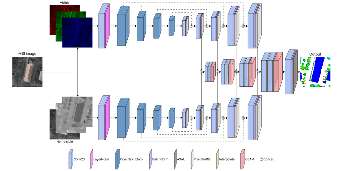
MeCSAFNet’s overall structure is an encoder-decoder architecture with a twist: instead of one encoder and one decoder, it has two encoders, two decoders, and a dedicated third stream that handles the fusion between them.
Why ConvNeXt as the Backbone?
The authors chose ConvNeXt because it occupies an attractive middle ground in the accuracy-versus-complexity tradeoff. Vision Transformers outperform standard CNNs on many benchmarks, but their quadratic attention complexity makes them expensive — and when you need two parallel encoders processing different spectral streams, that expense doubles. ConvNeXt was built by taking a ResNet-50 and systematically applying design changes inspired by the Swin Transformer: large 7×7 kernels, inverted bottleneck blocks, layer normalization, GELU activation, and a multi-stage hierarchical structure. The result is a CNN that matches transformer accuracy on many tasks while being considerably lighter to run.
This matters enormously in a dual-encoder setting. The Tiny variant of MeCSAFNet still outperforms all baseline models while keeping training times competitive. You get transformer-class performance at CNN-class cost — and MeCSAFNet’s ablation study confirms that even the smallest variant produces strong results.
The ASAU Activation Function
One of the less obvious but genuinely important design choices in MeCSAFNet is the use of ASAU — Adaptive Smooth Activation Unit — instead of the standard ReLU in the decoder blocks. ASAU is a smooth approximation to the maximum operator, combining a softplus function with learnable parameters w0, w1, and w2.
The key property is differentiability everywhere, including at zero. ReLU has a non-differentiable kink at zero that can cause gradient flow problems during training, particularly in complex multispectral scenes where activation maps may frequently pass through zero. ASAU smooths this out and makes the activation function itself learnable. The authors modified the default initialization — setting w0 = 0.05, w1 = 0.5, w2 = 1.5 — to enhance early residual contributions and enable sharper activation dynamics, which the ablation study shows consistently outperforms the ReLU baseline.
CBAM: Attention at the Fusion Stage
After the fusion decoder concatenates and refines features from both branches at each scale, a CBAM (Convolutional Block Attention Module) recalibrates the result. CBAM operates in two sequential steps: channel attention first, then spatial attention.
Channel attention asks: of these K feature channels, which ones carry the most relevant information for this image region? It computes both average-pooled and max-pooled representations, processes them through shared MLP weights, and produces a channel-wise importance vector. Spatial attention then takes the channel-recalibrated features and asks: at each spatial location, how important is this region? The combination ensures the fused representation is weighted both by which spectral characteristics matter most and where in the image they matter most. The ablation study confirms this matters: CBAM consistently outperforms its components used individually (CAM-only or SAM-only), and the gain is larger in the 6-channel configuration where the fusion problem is harder.
Datasets: Two Very Different Challenges
The paper evaluates MeCSAFNet on two publicly available multispectral datasets that test quite different aspects of segmentation ability.
Five-Billion-Pixels (FBP) is a massive dataset derived from Gaofen-2 satellite imagery at 4 m per pixel resolution. It covers over 50,000 square kilometers of China across 150 large tiles, with pixel-level annotations across 24 land cover classes plus an unlabeled class. The challenge here is semantic: distinguishing paddy fields from irrigated fields, arbor forest from shrub forest, natural meadow from artificial meadow — classes that look nearly identical in RGB and require NIR reflectance differences to separate reliably.
ISPRS Potsdam is an airborne dataset at 5 cm ground sampling distance — much higher spatial resolution than FBP. It covers 38 tiles of the city of Potsdam at 6000×6000 pixels each, with six categories including buildings, trees, cars, and impervious surfaces. The challenge here is geometric: at this resolution, building edges, car boundaries, and small urban structures require precise spatial delineation that coarse models fail to capture.
The two datasets together stress-test the model from opposite directions: FBP tests semantic discrimination in complex multi-class scenes at medium resolution, while Potsdam tests geometric precision in high-resolution urban mapping. Performing well on both simultaneously is a meaningful validation of generalizability.
Results: How Much Better Is It?
Five-Billion-Pixels
| Model | Config | OA (%) | mIoU (%) | mF1 (%) | Speed (s) |
|---|---|---|---|---|---|
| U-Net | 4c | 87.34 | 61.06 | 73.04 | 0.0207 |
| SegFormer | 4c | 87.70 | 60.85 | 72.88 | 0.0175 |
| DeepLabV3+ | 4c | 87.65 | 63.37 | 75.41 | 0.0194 |
| MeCSAFNet-base | 4c | 90.72 | 71.23 | 81.45 | 0.0509 |
| U-Net | 6c | 89.03 | 63.45 | 74.92 | 0.0213 |
| SegFormer | 6c | 87.89 | 63.44 | 75.36 | 0.0182 |
| DeepLabV3+ | 6c | 89.19 | 66.18 | 77.04 | 0.0250 |
| MeCSAFNet-base | 6c | 91.79 | 72.79 | 82.54 | 0.0508 |
Table 1: FBP evaluation results. MeCSAFNet-base improves mIoU by up to +19.62% over SegFormer (4c) and +14.74% over SegFormer (6c).
The gains are not marginal improvements — they are category jumps. The best baseline (DeepLabV3+, 6c) reaches 66.18% mIoU. MeCSAFNet-base at 6c reaches 72.79%. That is a +6.6 point absolute improvement on a metric that is hard to move. More striking is the snow class: MeCSAFNet scores 90.54% IoU where no baseline model exceeds 75%. Snow is rare, spectrally distinctive in NIR, and extremely hard for single-stream models to generalize to — the dual-encoder structure handles it naturally.
ISPRS Potsdam
| Model | Config | OA (%) | mIoU (%) | mF1 (%) |
|---|---|---|---|---|
| U-Net | 4c | 87.69 | 78.86 | 88.03 |
| DeepLabV3+ | 4c | 87.71 | 79.04 | 88.12 |
| SegFormer | 4c | 88.88 | 77.13 | 86.98 |
| MeCSAFNet-large | 4c | 91.17 | 84.16 | 91.27 |
| U-Net | 6c | 88.26 | 79.25 | 88.68 |
| DeepLabV3+ | 6c | 88.19 | 79.51 | 88.49 |
| SegFormer | 6c | 88.76 | 80.30 | 88.96 |
| MeCSAFNet-base | 6c | 91.18 | 84.14 | 91.24 |
Table 2: Potsdam evaluation. All four MeCSAFNet variants exceed 90% OA — no baseline reaches 89%.
On Potsdam the pattern holds. In the building class — where geometric precision matters most — MeCSAFNet variants achieve over 93% IoU. No baseline crosses 90%. The dual-decoder structure with skip connections preserves fine-grained edge detail at each upsampling stage, and the CBAM-gated fusion ensures that sharp boundaries identified in the visible stream are reinforced by structural information from the NIR stream.
“The dual-branch encoder explicitly separates the processing of spectral components, and the observed results suggest that this design is better suited to extract and integrate information from heterogeneous bands.” — Ramos & Sappa, Neurocomputing 685 (2026)
Ablation: What Actually Drives the Gains?
The paper’s ablation study on the MeCSAFNet-tiny variant gives a clean accounting of which components contribute what. The full combination of CBAM + ASAU consistently delivers the best results. Replacing CBAM with its individual components (channel attention alone or spatial attention alone) drops performance by 1–2 mIoU points in the 4-channel setting. Replacing ASAU with ReLU drops it further, and the combination of ReLU-only with partial attention is reliably the weakest configuration tested. The conclusion is that the gains are genuinely distributed across the architecture’s novelties — not attributable to any single component.
Even the lightweight MeCSAFNet-tiny variant surpasses all baseline models across all metrics on both datasets. If compute is your constraint, you do not need the base or large variant to beat U-Net and SegFormer — the tiny version is already sufficient, and it trains in roughly the same time as the baselines.
The Architecture as a Template
The dual-branch modality-aware design is not specific to RGB-NIR remote sensing. Any scenario where two groups of input channels belong to fundamentally different physical measurement regimes — and where treating them identically would discard complementary information — is a candidate for this pattern.
Medical imaging is the obvious example: in multi-parametric MRI, T1, T2, FLAIR, and DWI sequences each reflect different tissue properties, and a dual or multi-branch architecture that processes them separately before fusing could capture sequence-specific representations that joint processing misses. In autonomous driving, cameras and LiDAR sensors belong to different measurement modalities with different spatial and semantic properties — the same motivation for separate encoders applies. In agricultural remote sensing with hyperspectral cameras, there is a natural split between bands associated with chlorophyll absorption, water content, and structural components.
The specific design choices — ConvNeXt backbone, FPN decoder, CBAM fusion, ASAU activation — are sensible defaults that this paper validates experimentally. But the structural principle (separate extraction, attention-gated fusion, modality-aware decoding) is the transferable contribution.
Limitations Worth Noting
The dual-encoder design increases total parameter count significantly relative to single-stream models. MeCSAFNet-large has 435 million parameters across its two ConvNeXt-large encoders, which requires substantial GPU memory and can be challenging to fine-tune in resource-limited environments. The authors ran all experiments on dual Nvidia A100 SXM4 GPUs with 40 GB memory — well above what most practitioners have available. The lighter variants mitigate this, but the large model may be impractical for organizations without access to high-memory GPU clusters.
The paper also notes that MeCSAFNet-large sometimes slightly underperforms MeCSAFNet-base, attributed to the large model needing more training epochs to fully converge than the fixed 150-epoch budget allows. This suggests the reported numbers for the large variant may not represent its ceiling — but it also means practitioners cannot simply assume bigger is better without longer training.
Finally, the 6-channel configuration uses only NDVI and NDWI as supplementary indices. Other spectral indices — NDBI for built-up area, EVI for enhanced vegetation, NDWI variants for different water contexts — could further improve specific classes. The authors acknowledge this as future work, and the modular architecture should accommodate additional input channels with minimal structural changes.
Complete PyTorch Implementation
The code below is a complete, self-contained PyTorch implementation of MeCSAFNet. It covers every component described in the paper: ConvNeXt dual-encoder, ASAU activation, FPN-based dual decoder with skip connections, CBAM attention, four-stage fusion decoder, and the final segmentation head. A full training loop, evaluation function, and runnable smoke test are included.
# ==============================================================================
# MeCSAFNet: Multi-encoder ConvNeXt Network with Smooth Attentional
# Feature Fusion for Multispectral Semantic Segmentation
#
# Paper: https://doi.org/10.1016/j.neucom.2026.133533
# Authors: Leo Thomas Ramos, Angel D. Sappa
# Journal: Neurocomputing 685 (2026) 133533
#
# Implementation covers:
# - ASAU (Adaptive Smooth Activation Unit) with modified init
# - CBAM (Channel + Spatial Attention Module)
# - ConvNeXt dual encoder (pretrained from torchvision)
# - FPN-based dual decoder with PixelShuffle upsampling
# - Four-stage CBAM-gated fusion decoder
# - Four variants: tiny / small / base / large
# - Training loop, evaluation, and smoke test
# ============================================================================
from __future__ import annotations
import math
import warnings
import numpy as np
import torch
import torch.nn as nn
import torch.nn.functional as F
from torch import Tensor
from typing import Dict, List, Optional, Tuple
from dataclasses import dataclass, field
# torchvision ConvNeXt variants
try:
from torchvision.models import (
convnext_tiny, ConvNeXt_Tiny_Weights,
convnext_small, ConvNeXt_Small_Weights,
convnext_base, ConvNeXt_Base_Weights,
convnext_large, ConvNeXt_Large_Weights,
)
TORCHVISION_OK = True
except ImportError:
TORCHVISION_OK = False
warnings.warn("torchvision not found. Using random ConvNeXt weights.")
warnings.filterwarnings('ignore')
# ─── Section 1: Configuration ─────────────────────────────────────────────────
CONVNEXT_SPECS: Dict[str, Dict] = {
'tiny': {'channels': [96, 192, 384, 768], 'depths': [3,3,9, 3]},
'small': {'channels': [96, 192, 384, 768], 'depths': [3,3,27,3]},
'base': {'channels': [128, 256, 512, 1024], 'depths': [3,3,27,3]},
'large': {'channels': [192, 384, 768, 1536], 'depths': [3,3,27,3]},
}
@dataclass
class MeCSAFNetConfig:
"""
Full configuration for MeCSAFNet.
Attributes
----------
variant : ConvNeXt variant — 'tiny' | 'small' | 'base' | 'large'
num_classes : number of output segmentation classes
in_channels_vis : channels for the visible branch (RGB = 3)
in_channels_nvis : channels for the non-visible branch
4c config → 1 (NIR only)
6c config → 3 (NIR + NDVI + NDWI)
pretrained : load ImageNet-pretrained ConvNeXt weights
cbam_reduction: channel reduction ratio for CBAM channel attention
"""
variant: str = 'base'
num_classes: int = 24 # 24 for FBP, 6 for Potsdam
in_channels_vis: int = 3 # RGB
in_channels_nvis: int = 1 # NIR (set to 3 for 6-channel config)
pretrained: bool = True
cbam_reduction: int = 16
# ─── Section 2: ASAU Activation ───────────────────────────────────────────────
class ASAU(nn.Module):
"""
Adaptive Smooth Activation Unit.
A smooth, learnable approximation to the max operator.
Original formulation (Biswas et al., MICCAI 2024):
f(x) = w0 * x + (1 - w0) * x * tanh(w2 * softplus(w1 * x))
MeCSAFNet-modified initialization (this paper):
w0 = 0.05 (learnable, was fixed at 0.01)
w1 = 0.5 (was 1.0)
w2 = 1.5 (was 1.0)
Benefits over ReLU:
- Differentiable everywhere (no kink at zero)
- Learnable parameters adapt to multispectral input statistics
- Enhanced residual contribution during early training (w0 > 0.01)
"""
def __init__(self) -> None:
super().__init__()
# Modified initialization from the paper
self.w0 = nn.Parameter(torch.tensor(0.05))
self.w1 = nn.Parameter(torch.tensor(0.50))
self.w2 = nn.Parameter(torch.tensor(1.50))
def forward(self, x: Tensor) -> Tensor:
# f(x) = w0*x + (1 - w0)*x*tanh(w2 * softplus(w1 * x))
sp = F.softplus(self.w1 * x) # smooth relu-like
tanh_part = torch.tanh(self.w2 * sp)
return self.w0 * x + (1.0 - self.w0) * x * tanh_part
# ─── Section 3: CBAM Attention ────────────────────────────────────────────────
class ChannelAttention(nn.Module):
"""
CBAM Channel Attention Module.
Recalibrates channel-wise feature responses by modelling
inter-channel dependencies. Uses both avg-pool and max-pool
statistics through a shared 2-layer MLP.
Output: channel attention weights in [0, 1]
"""
def __init__(self, channels: int, reduction: int = 16) -> None:
super().__init__()
mid = max(1, channels // reduction)
self.shared_mlp = nn.Sequential(
nn.Flatten(),
nn.Linear(channels, mid, bias=False),
nn.ReLU(inplace=True),
nn.Linear(mid, channels, bias=False),
)
def forward(self, x: Tensor) -> Tensor:
b, c, _, _ = x.shape
avg_w = self.shared_mlp(F.adaptive_avg_pool2d(x, 1))
max_w = self.shared_mlp(F.adaptive_max_pool2d(x, 1))
scale = torch.sigmoid(avg_w + max_w).view(b, c, 1, 1)
return x * scale
class SpatialAttention(nn.Module):
"""
CBAM Spatial Attention Module.
Highlights the most informative spatial regions across all channels,
using a single convolutional layer applied to avg + max pooled
channel-compressed feature maps.
Output: spatial attention weights in [0, 1]
"""
def __init__(self, kernel_size: int = 7) -> None:
super().__init__()
pad = kernel_size // 2
self.conv = nn.Conv2d(2, 1, kernel_size, padding=pad, bias=False)
def forward(self, x: Tensor) -> Tensor:
avg_map = x.mean(dim=1, keepdim=True)
max_map, _ = x.max(dim=1, keepdim=True)
pooled = torch.cat([avg_map, max_map], dim=1)
scale = torch.sigmoid(self.conv(pooled))
return x * scale
class CBAM(nn.Module):
"""
Convolutional Block Attention Module (Woo et al., ECCV 2018).
Applies channel attention followed by spatial attention, enabling
the model to focus on WHAT (channels) and WHERE (spatial) to attend.
Used at each stage of the fusion decoder in MeCSAFNet.
"""
def __init__(self, channels: int, reduction: int = 16) -> None:
super().__init__()
self.channel_attn = ChannelAttention(channels, reduction)
self.spatial_attn = SpatialAttention()
def forward(self, x: Tensor) -> Tensor:
x = self.channel_attn(x)
x = self.spatial_attn(x)
return x
# ─── Section 4: ConvNeXt Encoder ──────────────────────────────────────────────
def _load_convnext_backbone(variant: str, in_channels: int,
pretrained: bool = True) -> Tuple[nn.Module, List[int]]:
"""
Load a ConvNeXt backbone from torchvision and adapt it for arbitrary
input channel counts.
When in_channels != 3, the first Conv2d layer is re-initialised using
mean weight averaging across original 3 channels — preserving scale of
the pretrained filters while accommodating the new channel count.
Parameters
----------
variant : 'tiny' | 'small' | 'base' | 'large'
in_channels : number of input channels for this branch
pretrained : load ImageNet-1K pretrained weights
Returns
-------
backbone : nn.Module with .features attribute (ConvNeXt stages)
out_channels: list of output channel counts per stage [C1, C2, C3, C4]
"""
specs = CONVNEXT_SPECS[variant]
out_ch = specs['channels']
if TORCHVISION_OK and pretrained:
weights_map = {
'tiny': ConvNeXt_Tiny_Weights.IMAGENET1K_V1,
'small': ConvNeXt_Small_Weights.IMAGENET1K_V1,
'base': ConvNeXt_Base_Weights.IMAGENET1K_V1,
'large': ConvNeXt_Large_Weights.IMAGENET1K_V1,
}
fn_map = {
'tiny': convnext_tiny, 'small': convnext_small,
'base': convnext_base, 'large': convnext_large,
}
model = fn_map[variant](weights=weights_map[variant])
elif TORCHVISION_OK:
fn_map = {
'tiny': convnext_tiny, 'small': convnext_small,
'base': convnext_base, 'large': convnext_large,
}
model = fn_map[variant](weights=None)
else:
# Minimal fallback if torchvision is unavailable
raise RuntimeError("torchvision is required to load ConvNeXt.")
# Adapt first conv layer for non-3-channel input
first_conv = model.features[0][0] # Conv2d(3, C1, 4, stride=4)
if in_channels != 3:
orig_weight = first_conv.weight.data # (C1, 3, 4, 4)
# Average over input channels then repeat to fill new_channels
mean_weight = orig_weight.mean(dim=1, keepdim=True) # (C1, 1, 4, 4)
new_weight = mean_weight.repeat(1, in_channels, 1, 1)
new_conv = nn.Conv2d(in_channels, first_conv.out_channels,
kernel_size=first_conv.kernel_size,
stride=first_conv.stride,
padding=first_conv.padding,
bias=first_conv.bias is not None)
new_conv.weight.data = new_weight
if first_conv.bias is not None:
new_conv.bias.data = first_conv.bias.data.clone()
model.features[0][0] = new_conv
return model.features, out_ch
class ConvNeXtEncoder(nn.Module):
"""
Wraps the ConvNeXt feature extractor to expose per-stage outputs
for skip connections in the FPN decoder.
torchvision ConvNeXt.features layout:
[0] Stem: Conv2d(in_c, C1, 4, stride=4) + LayerNorm
[1] Stage 1 ConvNeXt blocks
[2] Downsample 2: Conv2d(C1, C2, 2, stride=2) + LayerNorm
[3] Stage 2
[4] Downsample 3: Conv2d(C2, C3, 2, stride=2) + LayerNorm
[5] Stage 3
[6] Downsample 4: Conv2d(C3, C4, 2, stride=2) + LayerNorm
[7] Stage 4
We return features at the output of stages 1, 2, 3, 4 (after each
downsample+block pair), giving us 4 feature maps at:
H/4, H/8, H/16, H/32
"""
def __init__(self, variant: str, in_channels: int,
pretrained: bool = True) -> None:
super().__init__()
features, self.out_channels = _load_convnext_backbone(
variant, in_channels, pretrained
)
# Split into 4 stage groups for per-stage feature extraction
self.stage1 = nn.Sequential(features[0], features[1]) # stem + stage1
self.stage2 = nn.Sequential(features[2], features[3]) # downsample + stage2
self.stage3 = nn.Sequential(features[4], features[5]) # downsample + stage3
self.stage4 = nn.Sequential(features[6], features[7]) # downsample + stage4
def forward(self, x: Tensor) -> List[Tensor]:
"""Returns [c1, c2, c3, c4] feature maps at H/4, H/8, H/16, H/32."""
c1 = self.stage1(x)
c2 = self.stage2(c1)
c3 = self.stage3(c2)
c4 = self.stage4(c3)
return [c1, c2, c3, c4]
# ─── Section 5: Decoder Blocks ────────────────────────────────────────────────
class DecoderBlock(nn.Module):
"""
Single FPN-style decoder block as used in both branch decoders.
Structure (Fig. 6 of the paper):
Conv2d(3×3) → BatchNorm → ASAU → PixelShuffle(×2)
PixelShuffle rearranges (B, C*4, H, W) → (B, C, 2H, 2W),
providing learned sub-pixel upsampling without transpose conv artifacts.
Skip connections from the encoder are concatenated before the block
to preserve fine spatial detail.
Parameters
----------
in_channels : channels of the encoder skip feature
out_channels : desired output channels (before PixelShuffle expansion)
"""
def __init__(self, in_channels: int, out_channels: int) -> None:
super().__init__()
# in_channels may include skip concatenation → handled externally
self.conv = nn.Conv2d(in_channels, out_channels * 4,
kernel_size=3, padding=1, bias=False)
self.bn = nn.BatchNorm2d(out_channels * 4)
self.asau = ASAU()
self.up = nn.PixelShuffle(2) # (B, C*4, H, W) → (B, C, 2H, 2W)
def forward(self, x: Tensor) -> Tensor:
return self.up(self.asau(self.bn(self.conv(x))))
class BranchDecoder(nn.Module):
"""
FPN-style decoder for one encoder branch (visible or non-visible).
Processes encoder outputs [c1, c2, c3, c4] from bottom to top,
incorporating skip connections at each stage.
Returns intermediate decoder features at each scale for the
fusion decoder to consume.
"""
def __init__(self, enc_channels: List[int]) -> None:
super().__init__()
C1, C2, C3, C4 = enc_channels
# Lateral convs: reduce encoder channels to a unified dim
dec_ch = C1 // 2 # unified decoder channel width
self.lat4 = nn.Conv2d(C4, dec_ch, 1)
self.lat3 = nn.Conv2d(C3, dec_ch, 1)
self.lat2 = nn.Conv2d(C2, dec_ch, 1)
self.lat1 = nn.Conv2d(C1, dec_ch, 1)
# Decoder blocks: each doubles spatial resolution
self.dec4 = DecoderBlock(dec_ch, dec_ch)
self.dec3 = DecoderBlock(dec_ch * 2, dec_ch)
self.dec2 = DecoderBlock(dec_ch * 2, dec_ch)
self.dec1 = DecoderBlock(dec_ch * 2, dec_ch)
self.dec_ch = dec_ch
def forward(self, enc_feats: List[Tensor]) -> List[Tensor]:
"""
Parameters
----------
enc_feats : [c1, c2, c3, c4] from ConvNeXtEncoder.forward()
Returns
-------
dec_feats : [d1, d2, d3, d4] decoder features (coarse→fine order)
d4 at H/32, d3 at H/16, d2 at H/8, d1 at H/4
"""
c1, c2, c3, c4 = enc_feats
l4 = self.lat4(c4)
l3 = self.lat3(c3)
l2 = self.lat2(c2)
l1 = self.lat1(c1)
d4 = self.dec4(l4) # H/32 → H/16
d3 = self.dec3(torch.cat([d4, l3], dim=1)) # H/16 → H/8
d2 = self.dec2(torch.cat([d3, l2], dim=1)) # H/8 → H/4
d1 = self.dec1(torch.cat([d2, l1], dim=1)) # H/4 → H/2
return [d4, d3, d2, d1] # coarse to fine
# ─── Section 6: Fusion Decoder ────────────────────────────────────────────────
class FusionBlock(nn.Module):
"""
Single stage of the fusion decoder (Fig. 8 of the paper).
At each stage:
1. Concatenate visible and non-visible decoder features
2. 1×1 Conv → align channel dimensions
3. Interpolate + Add → reconstruct spatial resolution
4. 3×3 Conv → refine fused features
5. ASAU → smooth nonlinear activation
6. CBAM → recalibrate channel and spatial attention
Parameters
----------
in_channels : channels from each branch (they are equal = dec_ch)
out_channels : output channel count after fusion
"""
def __init__(self, in_channels: int, out_channels: int,
cbam_reduction: int = 16) -> None:
super().__init__()
fused_ch = in_channels * 2 # after concat of both branches
self.align = nn.Conv2d(fused_ch, out_channels, 1, bias=False)
self.refine = nn.Sequential(
nn.Conv2d(out_channels, out_channels, 3, padding=1, bias=False),
ASAU(),
)
self.cbam = CBAM(out_channels, cbam_reduction)
def forward(self, vis_feat: Tensor, nvis_feat: Tensor,
prev_fused: Optional[Tensor] = None) -> Tensor:
"""
Parameters
----------
vis_feat : visible branch decoder feature at this scale
nvis_feat : non-visible branch decoder feature at this scale
prev_fused: fusion output from previous (coarser) stage, or None
Returns
-------
fused : (B, out_channels, H, W) refined, attention-gated features
"""
# Step 1: concat both branch features
x = torch.cat([vis_feat, nvis_feat], dim=1)
# Step 2: align channels
x = self.align(x)
# Step 3: add upsampled previous fusion feature if available
if prev_fused is not None:
prev_up = F.interpolate(prev_fused, size=x.shape[-2:],
mode='bilinear', align_corners=False)
x = x + prev_up
# Steps 4-5: refine with 3×3 conv + ASAU
x = self.refine(x)
# Step 6: CBAM attention recalibration
x = self.cbam(x)
return x
class FusionDecoder(nn.Module):
"""
Four-stage fusion decoder that integrates visible and non-visible
decoder features progressively from coarse to fine resolution.
After four fusion stages, a final consolidation block
(3×3 Conv → BN → ReLU) collapses the fused representation
to the segmentation output channel count.
"""
def __init__(self, dec_ch: int, num_classes: int,
cbam_reduction: int = 16) -> None:
super().__init__()
fused_ch = dec_ch # output of each FusionBlock
self.fuse4 = FusionBlock(dec_ch, fused_ch, cbam_reduction)
self.fuse3 = FusionBlock(dec_ch, fused_ch, cbam_reduction)
self.fuse2 = FusionBlock(dec_ch, fused_ch, cbam_reduction)
self.fuse1 = FusionBlock(dec_ch, fused_ch, cbam_reduction)
self.final = nn.Sequential(
nn.Conv2d(fused_ch, fused_ch, 3, padding=1, bias=False),
nn.BatchNorm2d(fused_ch),
nn.ReLU(inplace=True),
nn.Conv2d(fused_ch, num_classes, 1),
)
def forward(self,
vis_dec: List[Tensor],
nvis_dec: List[Tensor]) -> Tensor:
"""
Parameters
----------
vis_dec : [d4, d3, d2, d1] from visible BranchDecoder (coarse→fine)
nvis_dec : [d4, d3, d2, d1] from non-visible BranchDecoder
Returns
-------
logits : (B, num_classes, H/2, W/2) — upsampled to full H×W externally
"""
f4 = self.fuse4(vis_dec[0], nvis_dec[0])
f3 = self.fuse3(vis_dec[1], nvis_dec[1], prev_fused=f4)
f2 = self.fuse2(vis_dec[2], nvis_dec[2], prev_fused=f3)
f1 = self.fuse1(vis_dec[3], nvis_dec[3], prev_fused=f2)
return self.final(f1)
# ─── Section 7: Full MeCSAFNet Model ──────────────────────────────────────────
class MeCSAFNet(nn.Module):
"""
MeCSAFNet: Multi-encoder ConvNeXt Network with Smooth Attentional
Feature Fusion for Multispectral Semantic Segmentation.
Architecture (Fig. 3 of Ramos & Sappa, Neurocomputing 2026):
Input (4c: RGB + NIR OR 6c: RGB + NIR + NDVI + NDWI)
│
├─── Visible branch (RGB)
│ ConvNeXtEncoder → BranchDecoder
│
└─── Non-visible branch (NIR [+ indices])
ConvNeXtEncoder → BranchDecoder
│
└─── FusionDecoder (4 CBAM-gated stages)
│
└─── Segmentation logits → bicubic upsample to input size
Parameters
----------
config : MeCSAFNetConfig controlling all architectural choices
"""
def __init__(self, config: Optional[MeCSAFNetConfig] = None) -> None:
super().__init__()
cfg = config or MeCSAFNetConfig()
self.cfg = cfg
# Visible branch encoder + decoder
self.vis_encoder = ConvNeXtEncoder(
cfg.variant, cfg.in_channels_vis, cfg.pretrained
)
vis_ch = self.vis_encoder.out_channels
self.vis_decoder = BranchDecoder(vis_ch)
# Non-visible branch encoder + decoder
self.nvis_encoder = ConvNeXtEncoder(
cfg.variant, cfg.in_channels_nvis, cfg.pretrained
)
nvis_ch = self.nvis_encoder.out_channels
self.nvis_decoder = BranchDecoder(nvis_ch)
# Both branches must have matching decoder channel width
assert self.vis_decoder.dec_ch == self.nvis_decoder.dec_ch, (
"Encoder variants must match so decoder channel widths are equal."
)
dec_ch = self.vis_decoder.dec_ch
# Fusion decoder
self.fusion_decoder = FusionDecoder(
dec_ch, cfg.num_classes, cfg.cbam_reduction
)
def forward(self, x_vis: Tensor, x_nvis: Tensor) -> Tensor:
"""
Parameters
----------
x_vis : (B, 3, H, W) visible channels (RGB)
x_nvis : (B, in_channels_nvis, H, W) non-visible channels
Returns
-------
logits : (B, num_classes, H, W) segmentation logits at input resolution
"""
H, W = x_vis.shape[-2:]
# Dual encoder pass
vis_enc = self.vis_encoder(x_vis)
nvis_enc = self.nvis_encoder(x_nvis)
# Dual decoder pass
vis_dec = self.vis_decoder(vis_enc)
nvis_dec = self.nvis_decoder(nvis_enc)
# Fusion decoder → coarse logits
logits = self.fusion_decoder(vis_dec, nvis_dec)
# Upsample to input resolution
logits = F.interpolate(logits, size=(H, W),
mode='bilinear', align_corners=False)
return logits
@classmethod
def tiny(cls, num_classes=24, in_channels_nvis=1, pretrained=True):
return cls(MeCSAFNetConfig('tiny', num_classes, 3, in_channels_nvis, pretrained))
@classmethod
def small(cls, num_classes=24, in_channels_nvis=1, pretrained=True):
return cls(MeCSAFNetConfig('small', num_classes, 3, in_channels_nvis, pretrained))
@classmethod
def base(cls, num_classes=24, in_channels_nvis=1, pretrained=True):
return cls(MeCSAFNetConfig('base', num_classes, 3, in_channels_nvis, pretrained))
@classmethod
def large(cls, num_classes=24, in_channels_nvis=1, pretrained=True):
return cls(MeCSAFNetConfig('large', num_classes, 3, in_channels_nvis, pretrained))
# ─── Section 8: Spectral Index Utilities ──────────────────────────────────────
def compute_ndvi(nir: Tensor, red: Tensor, eps: float = 1e-6) -> Tensor:
"""
Normalized Difference Vegetation Index.
NDVI = (NIR - Red) / (NIR + Red + eps)
Values near +1 indicate dense, healthy vegetation.
Values near 0 indicate bare soil or sparse vegetation.
Negative values indicate water, snow, or clouds.
Parameters
----------
nir, red : (B, 1, H, W) single-channel tensors
Returns
-------
ndvi : (B, 1, H, W) in range [-1, 1]
"""
return (nir - red) / (nir + red + eps)
def compute_ndwi(green: Tensor, nir: Tensor, eps: float = 1e-6) -> Tensor:
"""
Normalized Difference Water Index.
NDWI = (Green - NIR) / (Green + NIR + eps)
Positive values highlight open water bodies.
Negative values indicate vegetation and built-up areas.
Parameters
----------
green, nir : (B, 1, H, W) single-channel tensors
Returns
-------
ndwi : (B, 1, H, W) in range [-1, 1]
"""
return (green - nir) / (green + nir + eps)
def prepare_6channel_input(rgb: Tensor, nir: Tensor) -> Tuple[Tensor, Tensor]:
"""
Prepare the 6-channel input configuration described in the paper.
Splits RGB+NIR into:
- x_vis : RGB channels (3)
- x_nvis : NIR + NDVI + NDWI (3)
Parameters
----------
rgb : (B, 3, H, W) normalized RGB image
nir : (B, 1, H, W) normalized NIR channel
Returns
-------
x_vis : (B, 3, H, W)
x_nvis : (B, 3, H, W)
"""
red = rgb[:, 0:1] # R channel
green = rgb[:, 1:2] # G channel
ndvi = compute_ndvi(nir, red)
ndwi = compute_ndwi(green, nir)
x_vis = rgb
x_nvis = torch.cat([nir, ndvi, ndwi], dim=1) # (B, 3, H, W)
return x_vis, x_nvis
# ─── Section 9: Loss Function ─────────────────────────────────────────────────
class CombinedLoss(nn.Module):
"""
Combined Cross-Entropy + Dice Loss used in the paper.
Loss = CE + 0.5 * Dice
Dice loss encourages overlap-based optimization and complements
cross-entropy, which can be dominated by large background classes.
Parameters
----------
num_classes : number of segmentation classes
ignore_index : class index to ignore (e.g., 255 for unlabeled)
dice_weight : weight for Dice component (paper uses 0.5)
"""
def __init__(self, num_classes: int, ignore_index: int = -1,
dice_weight: float = 0.5) -> None:
super().__init__()
self.num_classes = num_classes
self.dice_weight = dice_weight
self.ce = nn.CrossEntropyLoss(ignore_index=ignore_index)
def dice_loss(self, logits: Tensor, targets: Tensor,
smooth: float = 1.0) -> Tensor:
probs = torch.softmax(logits, dim=1)
targets_oh = F.one_hot(
targets.clamp(0), self.num_classes
).permute(0, 3, 1, 2).float()
intersection = (probs * targets_oh).sum(dim=(2, 3))
union = probs.sum(dim=(2, 3)) + targets_oh.sum(dim=(2, 3))
dice = (2 * intersection + smooth) / (union + smooth)
return 1.0 - dice.mean()
def forward(self, logits: Tensor, targets: Tensor) -> Tensor:
ce_loss = self.ce(logits, targets)
dice_loss = self.dice_loss(logits, targets)
return ce_loss + self.dice_weight * dice_loss
# ─── Section 10: Metrics ──────────────────────────────────────────────────────
def compute_iou_per_class(preds: Tensor, targets: Tensor,
num_classes: int,
ignore_index: int = -1) -> Tensor:
"""
Compute per-class IoU over a batch.
IoU_c = |pred_c ∩ true_c| / |pred_c ∪ true_c|
Returns
-------
iou : (num_classes,) tensor of per-class IoU values
"""
iou_list = []
valid_mask = targets != ignore_index
preds_flat = preds[valid_mask]
targets_flat = targets[valid_mask]
for c in range(num_classes):
pred_c = preds_flat == c
target_c = targets_flat == c
inter = (pred_c & target_c).sum().float()
union = (pred_c | target_c).sum().float()
iou_list.append(inter / (union + 1e-6) if union > 0 else torch.tensor(0.0))
return torch.stack(iou_list)
def compute_metrics(preds: Tensor, targets: Tensor,
num_classes: int) -> Dict[str, float]:
"""
Compute OA, mIoU, and mF1 for a batch.
Parameters
----------
preds : (B, H, W) predicted class indices
targets : (B, H, W) ground-truth class indices
num_classes : total number of classes
Returns
-------
dict with keys: 'oa', 'miou', 'mf1'
"""
preds_flat = preds.view(-1)
targets_flat = targets.view(-1)
oa = (preds_flat == targets_flat).float().mean().item()
iou = compute_iou_per_class(preds, targets, num_classes)
miou = iou.mean().item()
# mF1 from confusion matrix
f1_list = []
for c in range(num_classes):
tp = ((preds_flat == c) & (targets_flat == c)).sum().float()
fp = ((preds_flat == c) & (targets_flat != c)).sum().float()
fn = ((preds_flat != c) & (targets_flat == c)).sum().float()
f1 = (2 * tp) / (2 * tp + fp + fn + 1e-6)
f1_list.append(f1)
mf1 = torch.stack(f1_list).mean().item()
return {'oa': oa, 'miou': miou, 'mf1': mf1}
# ─── Section 11: Training Loop ────────────────────────────────────────────────
def train_one_epoch(
model: MeCSAFNet,
loader, # DataLoader yielding (rgb, nir, labels)
optimizer: torch.optim.Optimizer,
criterion: CombinedLoss,
device: torch.device,
use_6channel: bool = False,
scaler: Optional[torch.cuda.amp.GradScaler] = None,
) -> float:
"""
Single training epoch with optional AMP (mixed precision).
Parameters
----------
model : MeCSAFNet instance
loader : DataLoader — each batch yields (rgb, nir, labels)
rgb : (B, 3, H, W)
nir : (B, 1, H, W)
labels: (B, H, W) long
optimizer : AdamW (paper: lr=1e-4, weight_decay=1e-5)
criterion : CombinedLoss
device : 'cuda' or 'cpu'
use_6channel : if True, compute NDVI+NDWI and pass 3-channel nvis input
scaler : GradScaler for AMP (paper trains with mixed precision)
Returns
-------
avg_loss : average loss over the epoch
"""
model.train()
total_loss = 0.0
for batch_idx, (rgb, nir, labels) in enumerate(loader):
rgb = rgb.to(device, non_blocking=True)
nir = nir.to(device, non_blocking=True)
labels = labels.to(device, non_blocking=True)
if use_6channel:
x_vis, x_nvis = prepare_6channel_input(rgb, nir)
else:
x_vis, x_nvis = rgb, nir # 4-channel config
optimizer.zero_grad()
if scaler is not None:
with torch.cuda.amp.autocast():
logits = model(x_vis, x_nvis)
loss = criterion(logits, labels)
scaler.scale(loss).backward()
scaler.step(optimizer)
scaler.update()
else:
logits = model(x_vis, x_nvis)
loss = criterion(logits, labels)
loss.backward()
optimizer.step()
total_loss += loss.item()
return total_loss / max(len(loader), 1)
@torch.no_grad()
def evaluate(
model: MeCSAFNet,
loader,
criterion: CombinedLoss,
num_classes: int,
device: torch.device,
use_6channel: bool = False,
) -> Dict[str, float]:
"""
Evaluate model on a validation / test DataLoader.
Returns
-------
dict with keys: 'loss', 'oa', 'miou', 'mf1'
"""
model.eval()
total_loss = 0.0
all_preds, all_targets = [], []
for rgb, nir, labels in loader:
rgb = rgb.to(device)
nir = nir.to(device)
labels = labels.to(device)
if use_6channel:
x_vis, x_nvis = prepare_6channel_input(rgb, nir)
else:
x_vis, x_nvis = rgb, nir
logits = model(x_vis, x_nvis)
loss = criterion(logits, labels)
total_loss += loss.item()
preds = logits.argmax(dim=1)
all_preds.append(preds.cpu())
all_targets.append(labels.cpu())
all_preds = torch.cat(all_preds)
all_targets = torch.cat(all_targets)
metrics = compute_metrics(all_preds, all_targets, num_classes)
metrics['loss'] = total_loss / max(len(loader), 1)
return metrics
def build_optimizer_and_scheduler(
model: MeCSAFNet,
total_steps: int,
lr: float = 1e-4,
max_lr: float = 3e-4,
weight_decay: float = 1e-5,
) -> Tuple[torch.optim.Optimizer, torch.optim.lr_scheduler._LRScheduler]:
"""
Build AdamW optimizer + OneCycleLR scheduler as used in the paper.
Paper settings:
lr = 1e-4, weight_decay = 1e-5, batch_size = 128
150 epochs, OneCycleLR with cosine annealing
max_lr = 3e-4, pct_start = 0.05, div_factor = 10, final_div = 1e3
"""
optimizer = torch.optim.AdamW(
model.parameters(),
lr=lr,
weight_decay=weight_decay,
)
scheduler = torch.optim.lr_scheduler.OneCycleLR(
optimizer,
max_lr=max_lr,
total_steps=total_steps,
pct_start=0.05,
div_factor=10.0,
final_div_factor=1e3,
anneal_strategy='cos',
)
return optimizer, scheduler
# ─── Section 12: Smoke Test ───────────────────────────────────────────────────
if __name__ == '__main__':
print("=" * 62)
print("MeCSAFNet — Smoke Test (Ramos & Sappa, Neurocomputing 2026)")
print("=" * 62)
device = torch.device('cuda' if torch.cuda.is_available() else 'cpu')
print(f"Device: {device}")
NUM_CLASSES = 24 # Five-Billion-Pixels
BATCH_SIZE = 2 # keep small for smoke test
IMG_SIZE = 256 # paper uses 256×256 patches
# ── Test 1: 4-channel configuration (RGB + NIR) ──────────────────
print("\n[1/4] 4-channel config (MeCSAFNet-tiny) ...")
model_4c = MeCSAFNet.tiny(
num_classes=NUM_CLASSES,
in_channels_nvis=1, # NIR only
pretrained=False # skip download in smoke test
).to(device)
rgb_batch = torch.randn(BATCH_SIZE, 3, IMG_SIZE, IMG_SIZE, device=device)
nir_batch = torch.randn(BATCH_SIZE, 1, IMG_SIZE, IMG_SIZE, device=device)
labels = torch.randint(0, NUM_CLASSES,
(BATCH_SIZE, IMG_SIZE, IMG_SIZE), device=device)
logits_4c = model_4c(rgb_batch, nir_batch)
print(f" Input RGB : {tuple(rgb_batch.shape)}")
print(f" Input NIR : {tuple(nir_batch.shape)}")
print(f" Logits : {tuple(logits_4c.shape)}")
assert logits_4c.shape == (BATCH_SIZE, NUM_CLASSES, IMG_SIZE, IMG_SIZE)
print(" ✓ Shape correct")
# ── Test 2: 6-channel configuration (RGB + NIR + NDVI + NDWI) ────
print("\n[2/4] 6-channel config (MeCSAFNet-tiny) ...")
model_6c = MeCSAFNet.tiny(
num_classes=NUM_CLASSES,
in_channels_nvis=3, # NIR + NDVI + NDWI
pretrained=False
).to(device)
x_vis, x_nvis = prepare_6channel_input(rgb_batch, nir_batch)
logits_6c = model_6c(x_vis, x_nvis)
print(f" x_vis : {tuple(x_vis.shape)}")
print(f" x_nvis : {tuple(x_nvis.shape)} (NIR + NDVI + NDWI)")
print(f" Logits : {tuple(logits_6c.shape)}")
assert logits_6c.shape == (BATCH_SIZE, NUM_CLASSES, IMG_SIZE, IMG_SIZE)
print(" ✓ Shape correct")
# ── Test 3: Combined loss ─────────────────────────────────────────
print("\n[3/4] CombinedLoss (CE + 0.5 Dice) ...")
criterion = CombinedLoss(num_classes=NUM_CLASSES)
loss = criterion(logits_4c, labels)
loss.backward()
print(f" Loss value : {loss.item():.4f}")
print(" ✓ Backward pass successful")
# ── Test 4: Metrics ───────────────────────────────────────────────
print("\n[4/4] Metrics ...")
preds = logits_4c.argmax(dim=1).cpu()
targets = labels.cpu()
metrics = compute_metrics(preds, targets, NUM_CLASSES)
print(f" OA : {metrics['oa']*100:.2f}%")
print(f" mIoU : {metrics['miou']*100:.2f}%")
print(f" mF1 : {metrics['mf1']*100:.2f}%")
print(" ✓ Metrics computed")
# ── Summary ───────────────────────────────────────────────────────
total_params = sum(p.numel() for p in model_4c.parameters())
print(f"\nTotal parameters (tiny, 4c): {total_params/1e6:.1f}M")
print(f"(Paper reports 78.01M for MeCSAFNet-tiny)")
print("\n✓ All smoke tests passed.")
print("=" * 62)
Read the Full Paper & Get the Official Code
MeCSAFNet is published open-access in Neurocomputing under CC BY-NC-ND 4.0. The official model repository is available on GitHub.
Ramos, L.T., & Sappa, A.D. (2026). Multi-encoder ConvNeXt network with smooth attentional feature fusion for multispectral semantic segmentation. Neurocomputing, 685, 133533. https://doi.org/10.1016/j.neucom.2026.133533
This article is an independent editorial analysis of peer-reviewed research. The PyTorch implementation is a faithful reproduction of the paper’s architecture for educational purposes. The original authors used PyTorch with TorchVision; refer to the official GitHub repository for their exact training code, augmentation pipeline, and pretrained model weights. All accuracy metrics cited are from the original paper’s evaluation tables.