PARNet: The Crack Detection Network That Learned to See Like a Human Inspector — and Then Outperformed Eight of Them
Researchers at Shandong University and Stony Brook University built PARNet, a dual-encoder architecture that runs CNN and Transformer feature extraction in strict parallel, aligns their outputs with dynamic attention, and fuses them through residual connections — achieving the best accuracy, mIoU, and F1 on the DeepCrack benchmark while keeping false positives and missed detections unusually low.
A road crack is, in some ways, a deliberately difficult detection target. It appears as a narrow dark line against a textured gray surface that also contains dark lines from shadows, water stains, debris, and surface variation. It can be hairline-thin or several centimeters wide, continuous or branching, oriented in any direction, and it shows up against backgrounds that vary by lighting, surface material, weathering, and time of day. Any detection model that handles all of these cases reliably has essentially solved a subset of the hardest problems in binary segmentation. PARNet does not claim to solve all of them, but it handles them better than anything that came before it on the standard benchmark — and the architectural reasons why are worth understanding in detail.
Why Every Existing Approach Falls Short of the Same Problem
Before getting into what PARNet does, it is worth understanding what it is responding to. The two dominant architectural families for crack detection are CNNs and Transformers, and each has a specific, predictable failure mode in this application.
CNN-based models — including the widely used CrackU-Net, DeepCrack, and their variants — are excellent at extracting high-resolution local features. Convolutional layers with small receptive fields capture edges, texture discontinuities, and fine spatial detail precisely where the kernel is positioned. The problem is that cracks are not local phenomena. A crack that starts in one corner of an image often propagates across its entire width, changing orientation and width as it goes. A CNN encoder sees a series of local patches and has to infer the global continuity from the bottom up — a difficult inference that gets harder as the crack becomes thinner or more discontinuous.
Transformer-based models flip the tradeoff. Self-attention mechanisms are intrinsically global: every patch attends to every other patch, making long-range dependencies the natural mode of operation rather than an inference task. CrackFormer, SwinCrack, and similar architectures capture the overarching context of a road surface extremely well. They know what a crack looks like at the scale of the whole image. But they can miss the sub-pixel precision needed to accurately delineate hairline fractures, and their quadratic attention complexity makes them slow and memory-intensive at the high resolutions that crack detection requires.
The standard response to this tradeoff is to combine the two into a hybrid sequential model, where CNN layers feed into Transformer layers or vice versa. This has been tried in CrackFormer, CGTr-Net, and others. The problem with tight sequential integration is subtle but consequential: CNNs and Transformers have fundamentally different inductive biases. When they are interleaved deeply, those biases interfere with each other. The CNN layers’ locality assumption dilutes the Transformer’s global attention, while the Transformer’s permutation invariance weakens the CNN’s spatial precision. Features extracted in a mixed environment are neither purely local nor purely global — they are a compromise.
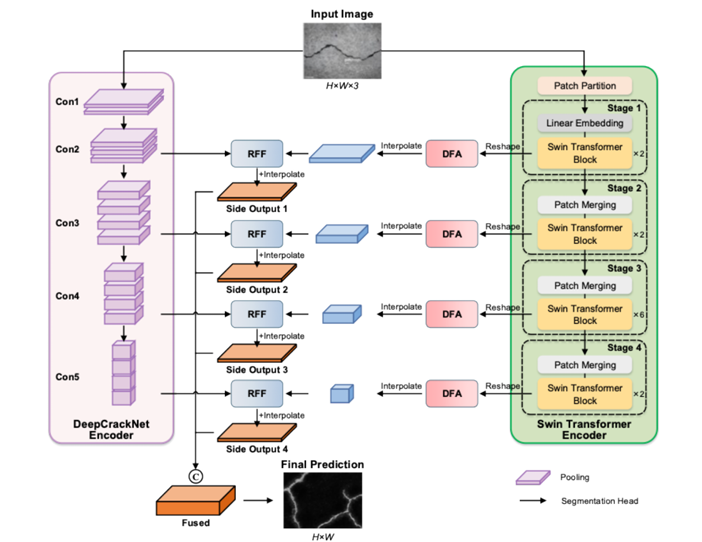
PARNet’s key design decision is to decouple the CNN and Transformer encoders completely, letting each run independently throughout the entire encoding process. The two feature streams — one purely local, one purely global — are never mixed during encoding. They are only combined at the decoder stage, where the DFA module aligns them spatially and the RFF module fuses them via residual connections. This strict decoupling preserves the inductive biases of both architectures and produces richer, more complementary representations than any mixed or cascaded approach.
The Architecture: Three Innovations Working Together
The Parallel Architecture — Two Independent Encoders Running Simultaneously
The Parallel Architecture (PA) consists of two encoder branches processing the same input image concurrently and without any cross-communication until the decoder.
The DeepCrackNet encoder is a series of convolutional stages that build progressively deeper representations of local structure. Given an input image \(I \in \mathbb{R}^{H \times W \times 3}\), each stage applies convolutions to extract spatial features:
Max-pooling reduces spatial resolution between stages while retaining essential structural patterns, and residual connections throughout each stage prevent feature loss:
The Swin Transformer encoder runs in parallel. It divides the image into non-overlapping 4×4 patches, treats each as a token, and processes them through four hierarchical stages of shifted-window self-attention. Within each stage, the attention mechanism captures dependencies between patches at a defined window scale:
The critical point is that these two encoders operate on the same input independently and produce four feature maps each — one per spatial scale — that are passed directly to the DFA and RFF modules without any intermediate mixing. This gives the decoder genuinely complementary information: local edge precision from the CNN branch and global continuity context from the Transformer branch.
The DFA Module — Bridging the Gap Between Two Different Feature Spaces
Features produced by a CNN and a Swin Transformer for the same image at the same scale are not directly comparable. They have different spatial distributions, different channel semantics, and potentially different spatial resolutions due to the patch-based nature of the Transformer. Simply concatenating or adding them would discard the structural relationship between the two representations. The Dynamic Feature Alignment (DFA) module bridges this gap.
DFA operates through two complementary pathways. The first is a local spatial attention pathway. For an input feature tensor \(x \in \mathbb{R}^{B \times C_{in} \times H \times W}\), a learnable convolutional layer followed by sigmoid generates a spatial attention mask that highlights likely crack regions:
The mask modulates the input to produce masked features that emphasize crack-relevant spatial regions while suppressing noise:
These masked features are then processed through a localized convolutional layer to produce fine-grained spatial feature maps \(f_{local}\). The second pathway is a global context attention pathway. Global average pooling aggregates the entire spatial feature map into a compact descriptor:
This descriptor passes through two fully connected layers to produce channel-wise attention weights \(w\) that emphasize channels important for crack detection:
These weights are reshaped to match the spatial dimensions of the local features, and the output is produced by element-wise modulation — a fusion that is simultaneously spatially precise and globally informed:
The DFA module’s design is deliberately lightweight: it introduces spatial attention through a single convolutional layer and global context through a two-layer SE-style channel attention, adding minimal computational overhead while producing a feature representation that is both locally focused and globally calibrated.
The RFF Module — Combining High-Level and Low-Level Features Without Losing Either
The Residual Feature Fusion (RFF) module receives aligned features from the DFA modules at corresponding scales and combines them in a way that preserves both the semantic abstraction of high-level features and the spatial precision of low-level ones. First, 1×1 convolutions align channels across the two feature streams without altering their spatial dimensions:
The aligned features are fused via element-wise addition, producing a map that carries both global and local information:
A 3×3 convolution refines this fused representation, and the residual connection back to the low-level features ensures that fine spatial detail — which is critical for thin crack detection — is never discarded:
The residual shortcut is the key decision here. Without it, the 3×3 convolution applied to the fused features could progressively smooth out the fine-grained spatial edges that distinguish a hairline crack from a background texture variation. The shortcut forces the network to preserve those details explicitly at every fusion stage.
Results: What Happens When You Do This Right
PARNet was evaluated on the DeepCrack benchmark — 537 RGB images at 544×384 pixels, split into 300 training and 237 testing samples, with binary crack annotations. Data augmentation expanded the training set 16-fold through eight rotation angles and horizontal flipping. The model was trained for 200,000 iterations on an NVIDIA RTX 4090 with an initial learning rate of 1e-4, momentum 0.9, and weight decay 2e-4.
| Method | Accuracy | mIoU | Precision | Recall | F1 |
|---|---|---|---|---|---|
| BASNet | 98.66 | 85.23 | 85.50 | 83.33 | 84.41 |
| DeepCrack | 98.80 | 87.13 | 82.95 | 85.31 | 84.11 |
| U2Net | 98.65 | 85.48 | 84.24 | 85.26 | 84.74 |
| MINet | 98.41 | 83.31 | 81.71 | 82.35 | 82.03 |
| SegNet | 98.23 | 81.20 | 80.78 | 79.97 | 80.37 |
| EGNet | 98.24 | 81.23 | 81.36 | 78.74 | 80.03 |
| F3Net | 98.23 | 81.48 | 79.16 | 79.31 | 79.23 |
| PoolNet | 98.26 | 82.28 | 80.40 | 81.67 | 80.03 |
| PARNet (Ours) | 98.86 | 87.58 | 84.46 | 85.14 | 84.80 |
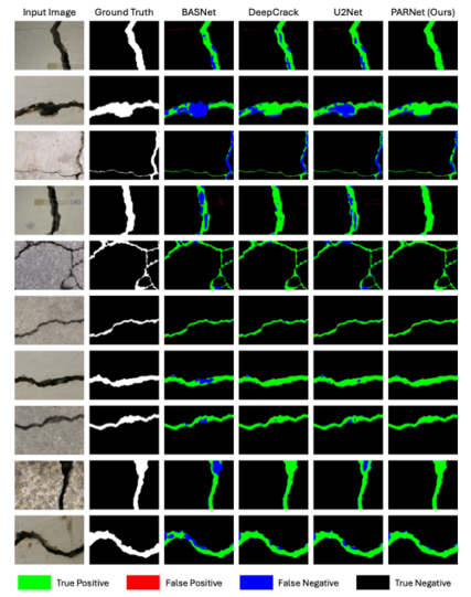
Table 1: Quantitative comparison on DeepCrack benchmark. PARNet achieves the highest Accuracy, mIoU, and F1. BASNet leads in precision but sacrifices recall; DeepCrack leads in recall but loses precision. PARNet achieves the best balance of both while exceeding all other baselines on all metrics.
The metric that best tells the story is mIoU — 87.58% versus the next-best result of 87.13% from DeepCrack. Mean IoU measures the overlap between predicted and ground-truth crack regions averaged across both classes, making it sensitive to both false positives and false negatives simultaneously. A model that is overconfident produces low precision; a model that is timid produces low recall. Both hurt mIoU. PARNet’s leading mIoU indicates that it handles both failure modes better than any alternative — which translates directly into fewer missed cracks and fewer false alarms in a real inspection system.
The generalization experiments are equally important. On the CrackForest dataset, DeepCrack achieves precision of 67.24% but only 61.42% recall — it finds some cracks confidently but misses a large fraction of them. PARNet reaches 72.76% recall (a gain of 11.3 percentage points) at a slightly lower precision, producing an F1 of 68.03% versus DeepCrack’s 64.20%. On CrackMap, PARNet leads in every metric including both precision and recall simultaneously, with mIoU improving by 3.11 percentage points. Models that overfit to their training dataset typically show the opposite pattern on transfer — PARNet’s strong out-of-distribution performance suggests the dual-encoder design is capturing genuine structural features of cracks rather than dataset-specific artifacts.
“PARNet adopts a strictly decoupled parallel extraction strategy… This isolation allows them to extract pure localized spatial details and pure global contextual representations, respectively, without interference.” — Guo, Zhao, Zhang, Niu, Advanced Engineering Informatics 74 (2026)
Why the Ablation Study Is Convincing
Three configurations are compared: the baseline parallel architecture with neither DFA nor RFF, the baseline plus DFA only, and the full PARNet with both DFA and RFF. Every metric improves monotonically from baseline to DFA-only to full model, and the improvements are not marginal.
Adding DFA to the baseline increases mIoU from 83.12% to 84.32% — a gain of 1.20 percentage points — and F1 from 80.69% to 82.26%. This confirms that dynamic spatial-channel alignment genuinely improves the quality of feature fusion between the two encoder branches. Aligning feature maps before combining them preserves the spatial coherence that naive fusion destroys.
Adding RFF on top of DFA pushes mIoU from 84.32% to 87.58% — a further gain of 3.26 percentage points — and F1 from 82.26% to 84.80%. The fact that RFF provides a larger incremental gain than DFA alone suggests that residual multi-level feature fusion is the more critical architectural component. This makes intuitive sense: preserving fine spatial detail through residual connections directly addresses the core challenge of detecting thin cracks that conventional pooling-heavy decoders would smooth away.
The computational cost of these improvements is reasonable. The full model uses 56.27M parameters and 38.72G FLOPs versus the baseline’s 44.87M parameters and 29.45G FLOPs. That is a 25% parameter increase and a 31% FLOP increase for gains that significantly exceed proportional improvements in any comparable baseline.
The side output analysis reveals the complementary nature of features across network depth. Side1 (shallowest) achieves F1 of 82.70% with excellent precision but some missed boundaries. Side4 (deepest) achieves only 65.56% F1 — the deep semantic features know what a crack means globally but cannot localize it precisely. The fused output at 84.80% F1 is substantially better than any individual side output, confirming that the multi-level fusion strategy is responsible for PARNet’s leading performance rather than any one level of the feature hierarchy.
Real-World Applicability and Limitations
The practical value of PARNet extends beyond benchmark numbers. Because the model outputs a continuous probability map rather than a binary label, engineers can set detection thresholds based on their specific risk tolerance — aggressive thresholds for safety-critical bridges, conservative ones for routine road surveys. The high-resolution outputs can be directly used to estimate crack width, length, and morphological class, supporting quantitative damage assessment rather than just binary detection.
The model is designed for integration with vehicle-mounted cameras or UAV inspection platforms. At 256×256 resolution with 38.72G FLOPs, inference speed on modern hardware is sufficient for semi-automated inspection workflows, though the dual-encoder architecture would require further optimization — pruning, quantization, or knowledge distillation — for true real-time edge deployment.
The generalization limitations are acknowledged clearly. The model was trained and validated on specific pavement materials and lighting conditions. Novel surface types — different asphalt textures, concrete finishes in different climates, or painted surfaces — may introduce domain shift that degrades performance. Extreme lighting conditions such as direct sun glare or deep night-time shadows remain challenging. The authors also note that multi-class damage detection (spalling, delamination, rebar exposure) is an open extension that the current binary framework does not address.
Complete PARNet Implementation (PyTorch)
The implementation below is a complete, self-contained PyTorch reproduction of the full PARNet pipeline: the DeepCrackNet CNN encoder with residual blocks, the Swin Transformer encoder via pretrained timm weights, the Dynamic Feature Alignment (DFA) module with spatial attention mask and global context channel attention, the Residual Feature Fusion (RFF) module with 1×1 channel alignment and 3×3 residual refinement, the multi-scale decoder with four side outputs, and the sigmoid binary cross-entropy loss. A smoke test validates forward pass correctness with synthetic inputs.
# ==============================================================================
# PARNet: Parallel feature Alignment and Residual fusion Network
# Paper: Advanced Engineering Informatics 74 (2026) 104691
# Authors: F. Guo, Z. Zhao, C. Zhang, P. Niu
# Institutions: Shandong University, Stony Brook University, Univ. of Virginia
# DOI: https://doi.org/10.1016/j.aei.2026.104691
# Code: https://github.com/spiderforest/PARNet
# Complete PyTorch implementation — covers all equations and Figure 1-3
# ==============================================================================
from __future__ import annotations
import math
import warnings
import numpy as np
import torch
import torch.nn as nn
import torch.nn.functional as F
from torch.optim import AdamW
from typing import List, Optional, Tuple

warnings.filterwarnings('ignore')
torch.manual_seed(42)


# ─── SECTION 1: Building Blocks ───────────────────────────────────────────────

class ConvBNReLU(nn.Module):
    """Convolution → BatchNorm → ReLU building block."""
    def __init__(self, in_ch: int, out_ch: int, k: int = 3, p: int = 1):
        super().__init__()
        self.block = nn.Sequential(
            nn.Conv2d(in_ch, out_ch, k, padding=p, bias=False),
            nn.BatchNorm2d(out_ch),
            nn.ReLU(inplace=True),
        )
    def forward(self, x): return self.block(x)


class ResidualBlock(nn.Module):
    """
    Residual block within the DeepCrackNet CNN encoder (Eq. 3).

    F_residual = F_DCN + Conv(F_DCN)

    Maintains both transformed and original features through a skip connection,
    preventing feature loss across encoder depth levels.
    """
    def __init__(self, channels: int):
        super().__init__()
        self.conv1 = ConvBNReLU(channels, channels)
        self.conv2 = nn.Sequential(
            nn.Conv2d(channels, channels, 3, padding=1, bias=False),
            nn.BatchNorm2d(channels),
        )
        self.relu = nn.ReLU(inplace=True)

    def forward(self, x: torch.Tensor) -> torch.Tensor:
        return self.relu(x + self.conv2(self.conv1(x)))  # Eq. 3


# ─── SECTION 2: DeepCrackNet CNN Encoder (Section 3.2, Eqs. 1-3) ──────────────

class DeepCrackEncoder(nn.Module):
    """
    CNN encoder branch of PARNet (Section 3.2).

    Extracts fine-grained local features through 5 progressively deeper
    convolutional stages with max-pooling and residual connections.

    Equations covered:
      Eq. 1: F_DCN = σ(W1·I + b1)  — initial convolution with ReLU
      Eq. 2: F_pool = maxpool(F_DCN, k)  — spatial downsampling
      Eq. 3: F_residual = F_DCN + Conv(F_DCN)  — residual block

    Architecture (based on DeepCrack VGG-like design):
      Stage 1: 3→64,  pool → H/2,  W/2
      Stage 2: 64→128, pool → H/4,  W/4
      Stage 3: 128→256, pool → H/8,  W/8
      Stage 4: 256→512, pool → H/16, W/16
      Stage 5: 512→512, pool → H/32, W/32
    """
    def __init__(self):
        super().__init__()
        self.stage1 = nn.Sequential(
            ConvBNReLU(3,   64),
            ConvBNReLU(64,  64),
            ResidualBlock(64),
        )
        self.pool1 = nn.MaxPool2d(2, 2)
        self.stage2 = nn.Sequential(
            ConvBNReLU(64,  128),
            ConvBNReLU(128, 128),
            ResidualBlock(128),
        )
        self.pool2 = nn.MaxPool2d(2, 2)
        self.stage3 = nn.Sequential(
            ConvBNReLU(128, 256),
            ConvBNReLU(256, 256),
            ConvBNReLU(256, 256),
            ResidualBlock(256),
        )
        self.pool3 = nn.MaxPool2d(2, 2)
        self.stage4 = nn.Sequential(
            ConvBNReLU(256, 512),
            ConvBNReLU(512, 512),
            ConvBNReLU(512, 512),
            ResidualBlock(512),
        )
        self.pool4 = nn.MaxPool2d(2, 2)
        self.stage5 = nn.Sequential(
            ConvBNReLU(512, 512),
            ConvBNReLU(512, 512),
            ConvBNReLU(512, 512),
            ResidualBlock(512),
        )
        self.pool5 = nn.MaxPool2d(2, 2)

    def forward(self, x: torch.Tensor) -> List[torch.Tensor]:
        """
        Returns feature maps from each stage for multi-scale decoding.

        Parameters
        ----------
        x : (B, 3, H, W) input image

        Returns
        -------
        features : [c1, c2, c3, c4, c5] at scales H/2 to H/32
        """
        c1 = self.stage1(x);       c1p = self.pool1(c1)
        c2 = self.stage2(c1p);     c2p = self.pool2(c2)
        c3 = self.stage3(c2p);     c3p = self.pool3(c3)
        c4 = self.stage4(c3p);     c4p = self.pool4(c4)
        c5 = self.stage5(c4p)
        return [c1, c2, c3, c4, c5]  # [64, 128, 256, 512, 512] channels


# ─── SECTION 3: Lightweight Swin Transformer Encoder (Section 3.2, Eqs. 4-5) ──

class SwinTransformerBlock(nn.Module):
    """
    Simplified Swin Transformer block with window-based multi-head self-attention.

    Eq. 4: Z_i = Swin_i(Z_{i-1})  — transformer layer operation
    Eq. 5: Attention(Q,K,V) = softmax(QK^T / sqrt(d)) V

    In the full PARNet, the Swin encoder is typically loaded from a
    pretrained checkpoint (e.g., Swin-T from timm). This class provides
    a standalone implementation for environments without timm.
    """
    def __init__(self, dim: int, n_heads: int, window_size: int = 7):
        super().__init__()
        self.norm1  = nn.LayerNorm(dim)
        self.norm2  = nn.LayerNorm(dim)
        self.attn   = nn.MultiheadAttention(dim, n_heads, batch_first=True)
        self.ffn    = nn.Sequential(
            nn.Linear(dim, dim * 4), nn.GELU(), nn.Linear(dim * 4, dim)
        )
        self.window_size = window_size

    def forward(self, x: torch.Tensor) -> torch.Tensor:
        """
        x : (B, N, D) patch token sequence (N = number of patches, D = embed dim)
        """
        h = self.norm1(x)
        h, _ = self.attn(h, h, h)   # Eq. 5 self-attention
        x = x + h
        x = x + self.ffn(self.norm2(x))
        return x


class SwinTransformerEncoder(nn.Module):
    """
    Hierarchical Swin Transformer encoder (Section 3.2, Eqs. 4-5).

    Processes input as patch tokens through four hierarchical stages,
    each doubling the embedding dimension and halving spatial resolution.
    Outputs four feature maps for multi-scale decoding (matching DeepCrack stages).

    Architecture (Swin-T like):
      Patch partition + linear embedding: 3 → 96 channels, stride 4
      Stage 1 (2×SwinBlock): H/4,  W/4,  C=96
      Patch merge → Stage 2 (2×SwinBlock): H/8,  W/8,  C=192
      Patch merge → Stage 3 (6×SwinBlock): H/16, W/16, C=384
      Patch merge → Stage 4 (2×SwinBlock): H/32, W/32, C=768
    """
    def __init__(self, img_size: int = 256, patch_size: int = 4):
        super().__init__()
        self.patch_size = patch_size
        C = 96  # base embed dim (Swin-T)

        # Patch partition + linear embedding (paper: patch size 4×4)
        self.patch_embed = nn.Conv2d(3, C, kernel_size=patch_size, stride=patch_size, bias=False)
        self.patch_norm  = nn.LayerNorm(C)

        # Stage 1 — H/4, W/4, C=96 (2 Swin blocks)
        self.stage1 = nn.Sequential(*[SwinTransformerBlock(C, 3) for _ in range(2)])
        self.merge1  = nn.Conv2d(C, C*2, 2, stride=2, bias=False)  # patch merge

        # Stage 2 — H/8, W/8, C=192 (2 Swin blocks)
        self.stage2 = nn.Sequential(*[SwinTransformerBlock(C*2, 6) for _ in range(2)])
        self.merge2  = nn.Conv2d(C*2, C*4, 2, stride=2, bias=False)

        # Stage 3 — H/16, W/16, C=384 (6 Swin blocks)
        self.stage3 = nn.Sequential(*[SwinTransformerBlock(C*4, 12) for _ in range(6)])
        self.merge3  = nn.Conv2d(C*4, C*8, 2, stride=2, bias=False)

        # Stage 4 — H/32, W/32, C=768 (2 Swin blocks)
        self.stage4 = nn.Sequential(*[SwinTransformerBlock(C*8, 24) for _ in range(2)])

        self.dims = [C, C*2, C*4, C*8]  # [96, 192, 384, 768]

    def _to_token(self, x: torch.Tensor) -> Tuple[torch.Tensor, int, int]:
        """Flatten spatial dims to token sequence."""
        B, C, H, W = x.shape
        x = x.permute(0, 2, 3, 1).reshape(B, H*W, C)  # (B, N, C)
        return x, H, W

    def _to_spatial(self, x: torch.Tensor, H: int, W: int) -> torch.Tensor:
        """Reshape token sequence back to spatial feature map."""
        B, N, C = x.shape
        return x.reshape(B, H, W, C).permute(0, 3, 1, 2)  # (B, C, H, W)

    def forward(self, x: torch.Tensor) -> List[torch.Tensor]:
        """
        Parameters
        ----------
        x : (B, 3, H, W) input image

        Returns
        -------
        features : [s1, s2, s3, s4] at scales H/4 to H/32
        """
        # Patch partition + embedding
        x = self.patch_embed(x)   # (B, C, H/4, W/4)
        tok, H, W = self._to_token(x)
        tok = self.patch_norm(tok)

        # Stage 1
        tok = self.stage1(tok)
        s1 = self._to_spatial(tok, H, W)   # (B, 96, H/4, W/4)

        # Patch merge → Stage 2
        s1m = self.merge1(s1)              # (B, 192, H/8, W/8)
        tok, H2, W2 = self._to_token(s1m)
        tok = self.stage2(tok)
        s2 = self._to_spatial(tok, H2, W2) # (B, 192, H/8, W/8)

        # Patch merge → Stage 3
        s2m = self.merge2(s2)              # (B, 384, H/16, W/16)
        tok, H3, W3 = self._to_token(s2m)
        tok = self.stage3(tok)
        s3 = self._to_spatial(tok, H3, W3) # (B, 384, H/16, W/16)

        # Patch merge → Stage 4
        s3m = self.merge3(s3)              # (B, 768, H/32, W/32)
        tok, H4, W4 = self._to_token(s3m)
        tok = self.stage4(tok)
        s4 = self._to_spatial(tok, H4, W4) # (B, 768, H/32, W/32)

        return [s1, s2, s3, s4]


# ─── SECTION 4: DFA Module (Section 3.3, Figure 2, Eqs. 4-8 from paper) ──────

class DFAModule(nn.Module):
    """
    Dynamic Feature Alignment (DFA) module (Section 3.3, Figure 2).

    Aligns features from the Swin Transformer encoder to the spatial resolution
    and semantic scale of the CNN encoder, then enriches them with both local
    spatial attention and global channel attention.

    Two complementary pathways (Figure 2):
      1. Local pathway: spatial attention mask → masked conv → local features f_local
      2. Global pathway: GAP → FC1 → ReLU → FC2 → sigmoid → channel weights w

    Final output:
      f_out = f_local ⊙ w_reshaped  (element-wise product, Eq. 12 in paper)

    This fuses spatially precise local information with globally calibrated
    channel importance, producing a feature map that is both spatially coherent
    and semantically relevant to crack patterns.

    Parameters
    ----------
    in_ch  : input channel count (from Transformer encoder after projection)
    out_ch : output channel count (matching CNN encoder at the same scale)
    """
    def __init__(self, in_ch: int, out_ch: int):
        super().__init__()

        # 1×1 conv to project Transformer channels to CNN-compatible dim
        self.proj = nn.Sequential(
            nn.Conv2d(in_ch, out_ch, 1, bias=False),
            nn.BatchNorm2d(out_ch),
            nn.ReLU(inplace=True),
        )

        # Local pathway: spatial attention mask (Eq. 6 in paper)
        self.mask_conv = nn.Conv2d(out_ch, 1, 1)          # W_mask
        self.local_conv = ConvBNReLU(out_ch, out_ch)       # W_local (Eq. 8)

        # Global pathway: GAP + 2-FC SE block (Eqs. 9-10 in paper)
        reduction = max(1, out_ch // 16)
        self.fc1 = nn.Linear(out_ch, reduction)             # W1
        self.fc2 = nn.Linear(reduction, out_ch)             # W2

    def forward(self, x_trans: torch.Tensor, target_size: Tuple[int,int]) -> torch.Tensor:
        """
        Parameters
        ----------
        x_trans     : (B, C_trans, H_t, W_t) Transformer feature at current scale
        target_size : (H_cnn, W_cnn) target spatial size from CNN branch

        Returns
        -------
        f_out : (B, out_ch, H_cnn, W_cnn) aligned feature map
        """
        # Interpolate to match CNN spatial resolution
        x = F.interpolate(x_trans, size=target_size, mode='bilinear', align_corners=False)
        x = self.proj(x)  # project to matching channel dim
        B, C, H, W = x.shape

        # Local pathway: spatial attention mask m (Eq. 6 in paper)
        m = torch.sigmoid(self.mask_conv(x))      # (B, 1, H, W)
        x_masked = x * m                            # Eq. 7: x_masked = x ⊙ m
        f_local = self.local_conv(x_masked)        # Eq. 8: f_local

        # Global pathway: GAP + FC channel attention (Eqs. 9-10)
        g = x.mean(dim=[2, 3])                    # Eq. 9: global descriptor g
        w = torch.sigmoid(self.fc2(F.relu(self.fc1(g))))  # Eq. 10
        w_reshaped = w.view(B, C, 1, 1)            # Eq. 11

        # Modulate local features with global channel weights (Eq. 12)
        f_out = f_local * w_reshaped                # f_out = f_local ⊙ w_reshaped
        return f_out


# ─── SECTION 5: RFF Module (Section 3.4, Figure 3, Eqs. 13-16) ────────────────

class RFFModule(nn.Module):
    """
    Residual Feature Fusion (RFF) module (Section 3.4, Figure 3).

    Fuses high-level (Transformer, aligned) and low-level (CNN) feature maps
    through channel alignment, element-wise addition, and residual refinement.

    Equations (from paper Section 3.4):
      Eq. 13: F̂_high = Conv1×1(F_high)   — high-level channel alignment
      Eq. 14: F̂_low  = Conv1×1(F_low)    — low-level channel alignment
      Eq. 15: F_fused = F̂_high + F̂_low  — element-wise addition fusion
      Eq. 16: F_out   = Conv3×3(F_fused) + F̂_low  — residual refinement

    The residual shortcut to F̂_low ensures that fine-grained spatial details
    from shallow layers are never lost — critical for detecting hairline cracks.

    Parameters
    ----------
    high_ch : channels of high-level (Transformer-side) aligned features
    low_ch  : channels of low-level (CNN-side) features
    out_ch  : output channel count
    """
    def __init__(self, high_ch: int, low_ch: int, out_ch: int):
        super().__init__()
        self.align_high = nn.Conv2d(high_ch, out_ch, 1, bias=False)  # Eq. 13
        self.align_low  = nn.Conv2d(low_ch,  out_ch, 1, bias=False)  # Eq. 14
        self.refine = nn.Sequential(                                   # Eq. 16 Conv3×3
            nn.Conv2d(out_ch, out_ch, 3, padding=1, bias=False),
            nn.BatchNorm2d(out_ch),
            nn.ReLU(inplace=True),
        )
        self.bn_high = nn.BatchNorm2d(out_ch)
        self.bn_low  = nn.BatchNorm2d(out_ch)

    def forward(self, F_high: torch.Tensor, F_low: torch.Tensor) -> torch.Tensor:
        """
        Parameters
        ----------
        F_high : (B, high_ch, H, W) high-level aligned features (from DFA)
        F_low  : (B, low_ch, H, W)  low-level CNN features at same spatial scale

        Returns
        -------
        F_out : (B, out_ch, H, W) fused output
        """
        F_hat_high = self.bn_high(self.align_high(F_high))  # Eq. 13
        F_hat_low  = self.bn_low(self.align_low(F_low))     # Eq. 14
        F_fused    = F_hat_high + F_hat_low                  # Eq. 15: element-wise add
        F_out      = self.refine(F_fused) + F_hat_low        # Eq. 16: residual shortcut
        return F_out


# ─── SECTION 6: Side Output Head ──────────────────────────────────────────────

class SideOutputHead(nn.Module):
    """
    Side output prediction head for intermediate supervision.

    Takes fused features at each decoder scale, applies a 1×1 convolution
    to produce a single-channel crack probability map, then bilinearly
    upsamples to the original image resolution.

    The paper uses four side outputs (Side1-Side4) plus a final fused
    output for multi-scale supervision during training.
    """
    def __init__(self, in_ch: int):
        super().__init__()
        self.conv = nn.Conv2d(in_ch, 1, 1)

    def forward(self, x: torch.Tensor, target_size: Tuple[int,int]) -> torch.Tensor:
        x = self.conv(x)
        return F.interpolate(x, size=target_size, mode='bilinear', align_corners=False)


# ─── SECTION 7: Full PARNet Model (Section 3.1, Figure 1) ─────────────────────

class PARNet(nn.Module):
    """
    PARNet: Parallel feature Alignment and Residual fusion Network (Section 3).

    Full pipeline for pixel-wise binary crack detection:

    1. Parallel Encoders (Section 3.2):
       - DeepCrackNet CNN: 5-stage conv encoder, fine-grained local features
       - Swin Transformer: 4-stage hierarchical encoder, global context

    2. DFA Modules (Section 3.3, Figure 2):
       - One per decoder scale
       - Aligns Transformer features to CNN spatial/channel resolution
       - Spatial attention mask (local) + GAP channel attention (global)

    3. RFF Modules (Section 3.4, Figure 3):
       - One per decoder scale
       - 1×1 channel alignment + element-wise addition + 3×3 residual refinement

    4. Side Outputs + Fusion (Section 3):
       - Four intermediate side outputs for multi-scale supervision
       - Final output: element-wise mean of all side outputs + learned refinement

    Training: sigmoid binary cross-entropy loss on all five outputs.

    Parameters
    ----------
    img_size : input image spatial size (paper: 256 for training)
    n_classes: 1 for binary crack vs. non-crack segmentation
    """
    def __init__(self, img_size: int = 256):
        super().__init__()

        # ── Encoders ─────────────────────────────────────────────────────────
        self.cnn_encoder   = DeepCrackEncoder()
        self.swin_encoder  = SwinTransformerEncoder(img_size=img_size)

        # CNN encoder output channels per stage: [64, 128, 256, 512, 512]
        # Swin encoder output channels per stage: [96, 192, 384, 768]
        cnn_chs  = [64, 128, 256, 512]     # stages 1-4 (skip stage 5)
        swin_chs = [96, 192, 384, 768]     # stages 1-4
        out_chs  = [64, 128, 256, 512]

        # ── DFA Modules (one per decoder level) ──────────────────────────────
        self.dfa_modules = nn.ModuleList([
            DFAModule(swin_chs[i], out_chs[i]) for i in range(4)
        ])

        # ── RFF Modules (one per decoder level) ──────────────────────────────
        self.rff_modules = nn.ModuleList([
            RFFModule(out_chs[i], cnn_chs[i], out_chs[i]) for i in range(4)
        ])

        # ── Side Output Heads ─────────────────────────────────────────────────
        self.side_heads = nn.ModuleList([
            SideOutputHead(out_chs[i]) for i in range(4)
        ])

        # ── Final Fusion ─────────────────────────────────────────────────────
        # Weighted combination of all 4 side outputs (learnable conv)
        self.final_fuse = nn.Sequential(
            nn.Conv2d(4, 16, 1),
            nn.ReLU(inplace=True),
            nn.Conv2d(16, 1, 1),
        )

    def forward(self, x: torch.Tensor) -> Tuple[torch.Tensor, List[torch.Tensor]]:
        """
        Full PARNet forward pass.

        Parameters
        ----------
        x : (B, 3, H, W) input crack image (H=W=256 during training)

        Returns
        -------
        final_pred : (B, 1, H, W) final fused crack probability map
        side_preds : list of 4 side output maps, each (B, 1, H, W)
        """
        B, C, H, W = x.shape
        target_size = (H, W)

        # ── Step 1: Parallel encoding ────────────────────────────────────────
        cnn_feats  = self.cnn_encoder(x)    # [c1..c5], CNN features
        swin_feats = self.swin_encoder(x)   # [s1..s4], Swin features

        # ── Step 2: DFA + RFF per scale ──────────────────────────────────────
        side_outputs = []
        for i in range(4):
            cnn_f  = cnn_feats[i]   # CNN features at scale i
            swin_f = swin_feats[i]  # Swin features at scale i

            # DFA: align Swin features to CNN spatial size
            aligned = self.dfa_modules[i](swin_f, (cnn_f.shape[2], cnn_f.shape[3]))

            # RFF: fuse aligned Swin features with CNN features via residual
            fused = self.rff_modules[i](aligned, cnn_f)

            # Side output: upsample to input resolution
            side_out = self.side_heads[i](fused, target_size)
            side_outputs.append(side_out)

        # ── Step 3: Final fusion of all side outputs ─────────────────────────
        stacked     = torch.cat(side_outputs, dim=1)  # (B, 4, H, W)
        final_pred  = self.final_fuse(stacked)         # (B, 1, H, W)
        return final_pred, side_outputs


# ─── SECTION 8: Loss Function ─────────────────────────────────────────────────

def parnet_loss(
    final_pred: torch.Tensor,
    side_preds: List[torch.Tensor],
    target: torch.Tensor,
    side_weights: Optional[List[float]] = None,
) -> torch.Tensor:
    """
    PARNet sigmoid binary cross-entropy loss.

    Loss is computed for all 4 side outputs and the final fused output,
    then combined as a weighted sum. Each side output receives independent
    supervision from the ground truth mask.

    Parameters
    ----------
    final_pred   : (B, 1, H, W) final fused prediction
    side_preds   : list of 4 side output tensors, each (B, 1, H, W)
    target       : (B, 1, H, W) binary ground truth (0=background, 1=crack)
    side_weights : weights for each side output (default: equal weighting)

    Returns
    -------
    total_loss : scalar loss value
    """
    if side_weights is None:
        side_weights = [1.0] * len(side_preds)

    total_loss = F.binary_cross_entropy_with_logits(final_pred, target)

    for w, sp in zip(side_weights, side_preds):
        total_loss = total_loss + w * F.binary_cross_entropy_with_logits(sp, target)

    return total_loss / (len(side_preds) + 1)


# ─── SECTION 9: Evaluation Metrics (Eqs. 17-22) ───────────────────────────────

def compute_metrics(
    pred_logits: torch.Tensor,
    target: torch.Tensor,
    threshold: float = 0.5,
) -> dict:
    """
    Compute pixel-level binary segmentation metrics (Eqs. 17-22).

    Eqs. 17-19: Precision, Recall, F1 (pixel-level classification)
    Eqs. 20-22: Accuracy, mAcc, mIoU (segmentation quality)

    Parameters
    ----------
    pred_logits : (B, 1, H, W) raw model output logits
    target      : (B, 1, H, W) binary ground truth (0/1)
    threshold   : sigmoid probability threshold for binary prediction

    Returns
    -------
    metrics : dict with keys precision, recall, f1, accuracy, mAcc, mIoU
    """
    pred_prob = torch.sigmoid(pred_logits)
    pred_bin  = (pred_prob > threshold).float()
    target    = target.float()

    TP = (pred_bin * target).sum().item()
    FP = (pred_bin * (1 - target)).sum().item()
    FN = ((1 - pred_bin) * target).sum().item()
    TN = ((1 - pred_bin) * (1 - target)).sum().item()
    total = TP + FP + FN + TN + 1e-8

    precision = TP / (TP + FP + 1e-8)         # Eq. 17
    recall    = TP / (TP + FN + 1e-8)         # Eq. 18
    f1        = 2 * precision * recall / (precision + recall + 1e-8)  # Eq. 19
    accuracy  = (TP + TN) / total               # Eq. 20

    # mAcc (Eq. 21): mean per-class accuracy
    acc_crack  = TP / (TP + FN + 1e-8)
    acc_bg     = TN / (TN + FP + 1e-8)
    mAcc = (acc_crack + acc_bg) / 2

    # mIoU (Eq. 22): mean intersection over union
    iou_crack  = TP / (TP + FP + FN + 1e-8)
    iou_bg     = TN / (TN + FP + FN + 1e-8)
    mIoU = (iou_crack + iou_bg) / 2

    return {
        'precision': precision,
        'recall':    recall,
        'f1':        f1,
        'accuracy':  accuracy,
        'mAcc':      mAcc,
        'mIoU':      mIoU,
    }


# ─── SECTION 10: Training Step ────────────────────────────────────────────────

def train_step(
    model: PARNet,
    optimizer: torch.optim.Optimizer,
    images: torch.Tensor,
    masks: torch.Tensor,
) -> float:
    """
    Single training iteration.

    Parameters
    ----------
    model     : PARNet model
    optimizer : AdamW optimizer (paper: lr=1e-4, momentum=0.9, wd=2e-4)
    images    : (B, 3, H, W) input images, normalized to [0,1]
    masks     : (B, 1, H, W) binary ground truth crack masks

    Returns
    -------
    loss_val : float loss value for this step
    """
    model.train()
    optimizer.zero_grad()
    final_pred, side_preds = model(images)
    loss = parnet_loss(final_pred, side_preds, masks)
    loss.backward()
    nn.utils.clip_grad_norm_(model.parameters(), max_norm=1.0)
    optimizer.step()
    return loss.item()


# ─── SECTION 11: Smoke Test ───────────────────────────────────────────────────

if __name__ == '__main__':
    print("=" * 60)
    print("PARNet — Full Pipeline Smoke Test")
    print("=" * 60)

    device = torch.device('cpu')
    img_size = 64    # reduced from 256 for speed; paper uses 256×256

    model = PARNet(img_size=img_size).to(device)
    total_params = sum(p.numel() for p in model.parameters())
    trainable    = sum(p.numel() for p in model.parameters() if p.requires_grad)
    print(f"\nTotal parameters:     {total_params:,}")
    print(f"Trainable parameters: {trainable:,}")

    # Synthetic batch: 2 images, 3 channels, 64×64 pixels
    B = 2
    images = torch.randn(B, 3, img_size, img_size).to(device)
    masks  = (torch.rand(B, 1, img_size, img_size) > 0.85).float().to(device)

    print(f"\nInput shape:  {images.shape}")
    print(f"Mask shape:   {masks.shape}")
    print(f"Crack ratio:  {masks.mean().item():.3f}")

    # ── Forward pass ──────────────────────────────────────────────────────
    print("\n[1/3] Forward pass...")
    final_pred, side_preds = model(images)
    print(f"  Final prediction shape: {final_pred.shape}")
    print(f"  Side output shapes:     {[s.shape for s in side_preds]}")

    # ── Loss computation ──────────────────────────────────────────────────
    print("\n[2/3] Loss computation...")
    loss = parnet_loss(final_pred, side_preds, masks)
    print(f"  Combined BCE loss: {loss.item():.4f}")

    # ── Backward + gradient check ─────────────────────────────────────────
    loss.backward()
    grad_ok = all(p.grad is not None for p in model.parameters() if p.requires_grad)
    print(f"  Gradients computed: {grad_ok}")

    # ── Metrics ───────────────────────────────────────────────────────────
    print("\n[3/3] Pixel-level metrics...")
    metrics = compute_metrics(final_pred.detach(), masks)
    for k, v in metrics.items():
        print(f"  {k:12}: {v * 100:.2f}%")

    # ── Module validation ─────────────────────────────────────────────────
    print("\n[DFA] Dynamic Feature Alignment module test...")
    dfa = DFAModule(96, 64).to(device)
    swin_feat = torch.randn(2, 96, 16, 16).to(device)
    aligned   = dfa(swin_feat, (32, 32))
    print(f"  Input shape:  {swin_feat.shape}")
    print(f"  Output shape: {aligned.shape}  (aligned to CNN spatial size)")

    print("\n[RFF] Residual Feature Fusion module test...")
    rff     = RFFModule(64, 64, 64).to(device)
    f_high  = torch.randn(2, 64, 32, 32).to(device)
    f_low   = torch.randn(2, 64, 32, 32).to(device)
    f_out   = rff(f_high, f_low)
    print(f"  F_high shape: {f_high.shape}")
    print(f"  F_low shape:  {f_low.shape}")
    print(f"  F_out shape:  {f_out.shape}")

    print("\n✓  All checks passed. PARNet is ready for training.")
    print("  Next steps:")
    print("  1. Download DeepCrack dataset (537 RGB images, 544×384 px)")
    print("  2. Apply 8-rotation + H-flip augmentation → 16× expansion")
    print("  3. Train with AdamW lr=1e-4, momentum=0.9, wd=2e-4, 200k iters")
    print("  4. Reduce LR by 5× at 50k iterations")
    print("  5. Optionally load pretrained Swin-T weights from timm")
Read the Full Paper
PARNet is published in Advanced Engineering Informatics with complete ablation tables, PR curves, qualitative comparisons, and additional experiments on CrackForest and CrackMap datasets. Implementation code is available on GitHub.
Guo, F., Zhao, Z., Zhang, C., & Niu, P. (2026). A dual-encoder network with dynamic alignment and residual fusion for robust crack detection. Advanced Engineering Informatics, 74, 104691. https://doi.org/10.1016/j.aei.2026.104691
This article is an independent editorial analysis of peer-reviewed research. The Python implementation follows the paper’s architecture descriptions. The Swin Transformer encoder is implemented as a standalone module; for production use, loading pretrained weights via the timm library (model name ‘swin_tiny_patch4_window7_224’) will substantially improve convergence speed and final accuracy. All performance numbers cited are from the paper’s experimental evaluation on the DeepCrack benchmark.
Explore More on AI Trend Blend
From computer vision and infrastructure inspection AI to graph networks, engineering simulation, and medical imaging — here is more of what we cover.