Teaching an AI to Care More About the Rarest Cancers: Class-Weighted DQN for Skin Cancer Classification
Researchers from KTO Karatay University and Selcuk University flipped the standard deep learning script — instead of augmenting their way out of class imbalance, they rewired the reward system of a Deep Q-Network so that correctly identifying a rare Dermatofibroma earns almost ten times more reward than correctly labeling the dominant Melanocytic Nevi, hitting 97.97% accuracy on the raw, unaugmented HAM10000 dataset.
Melanoma has a 98.4% survival rate when caught at stage 0 or I. By stage IV, that drops to 22.5%. The difference between those two numbers often comes down to whether a suspicious mole is correctly flagged — and correctly flagging it is harder than it sounds when the dataset used to train the AI has over 6,700 images of one benign class and only 115 images of a rare vascular lesion. Standard deep learning models learn the obvious lesson: always guess the majority class. This paper asks what happens when you train an RL agent to treat a rare correct guess as genuinely more valuable than a common one. The answer is a system that outperforms five contemporary transfer learning and CNN-based approaches across every metric, without touching a single data augmentation tool.
Why Class Imbalance Is a Clinical Problem, Not Just a Technical One
The HAM10000 dataset — the largest publicly available skin cancer dataset at the time of publication, from Harvard University — contains 10,015 dermoscopic images across seven diagnostic categories. On paper, 10,015 images sounds like a reasonable training set. In practice, the distribution looks like this: Melanocytic Nevi (NEV) alone accounts for nearly 67% of all images. Every other class shares the remaining 33%, with Dermatofibroma (DF) holding just 1.14% and Vascular lesions (VASC) at 1.42%.
When a standard neural network trains on this data, it quickly discovers that predicting NEV is almost always a safe bet. The loss function rewards accuracy, and predicting the majority class keeps accuracy high. The model converges toward a strategy that is mathematically optimal for the training objective but clinically dangerous — it will confidently miss the rare melanoma or vascular lesion every single time.
The usual fixes are data augmentation (synthesizing more minority-class examples) and class reweighting in the loss function (penalizing majority-class errors more). Both work to varying degrees. But the paper’s argument is that these approaches treat the symptom rather than the cause: they still use a static learning paradigm that cannot dynamically adjust its focus as training progresses. Reinforcement learning offers something different — a reward signal that can be designed from scratch to reflect clinical priorities.
In a class-weighted DQN, the reward the agent receives for a correct prediction is not a flat +1. It is inversely proportional to how common that class is in the dataset. Correctly classifying a Dermatofibroma — which comprises just 1.14% of the data — earns a reward of 0.9886. Correctly classifying Melanocytic Nevi — which is 66.95% of the data — earns only 0.3305. The agent learns, over thousands of episodes, that getting the rare cases right is what actually builds up its total score.
The Seven Skin Cancer Classes in HAM10000
Before diving into the architecture, it’s worth understanding what the model is actually trying to distinguish. The HAM10000 dataset contains seven clinically distinct categories, each with very different visual characteristics and levels of danger. Melanoma (MEL) is the most lethal — it originates in melanocytes and is responsible for roughly 9,000 deaths annually in the US alone. Melanocytic Nevi (NEV) are common benign moles that can look visually similar to early melanoma, making the classification boundary particularly treacherous. Basal Cell Carcinoma (BCC) is the most common skin cancer overall but rarely metastasizes. Actinic Keratoses and Intraepithelial Carcinoma (AKIEC) are precancerous lesions. Benign Keratosis-like lesions (BKL), Dermatofibroma (DF), and Vascular lesions (VASC) complete the set.
The epidemiology of the dataset also reveals something clinically interesting: skin cancer concentration increases sharply in patients aged 30 and above, peaks around 40–50, then tapers off. BKL, BCC, and AKIEC are heavily concentrated in patients aged 50–70. VASC is uniquely wide-ranging, appearing from the late 30s to early 70s. Males show higher lesion counts in almost every category, with the back being the most affected body site and the scalp and ears least affected.
The Class-Weighted Reward Design
The mathematical elegance of this paper is in how simple the reward function is. For any cancer class C, let Cp be the percentage composition of that class in the dataset (expressed as a fraction between 0 and 1). The positive reward for correctly classifying that class is:
The result is a symmetric, elegant mechanism: classes that are abundant in the data produce low positive rewards and low negative penalties. Classes that are rare produce high positive rewards and high negative penalties. The agent is therefore far more motivated to learn the rare classes — every correct rare classification meaningfully boosts its cumulative score, and every missed rare classification costs very little, while every missed common classification actually hurts more in absolute terms.
Here is what the reward table looks like for the full HAM10000 dataset:
The DQN Framework: How It Works
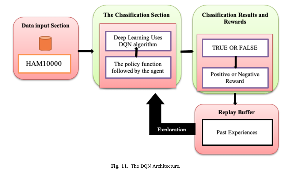
Deep Q-Learning (DQN) is a reinforcement learning algorithm that approximates the optimal Q-function — the function that maps a state and action pair to the expected cumulative reward — using a deep neural network. In the standard RL loop, an agent observes the current state of the environment, selects an action, receives a reward, and transitions to a new state. By repeating this over thousands of episodes, the agent builds up a policy that maximizes total reward.
Translated to skin cancer classification, the mapping is straightforward. The state is the current dermoscopic image (flattened to a pixel vector). The action is the predicted cancer class (one of seven). The reward is the class-weighted value defined above. The environment is the dataset itself — images are sampled stochastically, one batch per time step.
ENVIRONMENT (HAM10000 Dataset)
         │
         │  State: image pixels (28×28×3 = 2,352 features)
         ▼
┌────────────────────────────────────────────────────────┐
│  DQN AGENT (Multi-Layer Perceptron)                    │
│                                                        │
│  Input Layer   →  2,352 neurons (flattened RGB image)  │
│  Hidden Layer  →  fully connected, ReLU activation     │
│  Output Layer  →  7 neurons (Q-values per class)       │
│                                                        │
│  ε-greedy Policy: explore OR exploit                   │
│    - With prob. ε: pick random action (explore)        │
│    - With prob. 1-ε: pick argmax Q-value (exploit)     │
└──────────┬─────────────────────────────────────────────┘
           │  Action: predicted class {A0…A6}
           ▼
┌────────────────────────────────────────────────────────┐
│  REWARD COMPUTATION                                    │
│                                                        │
│  Correct?  →  Rp = 1 − Cp  (rare class = high reward) │
│  Wrong?    →  Rn = −Cp     (rare miss = small penalty) │
└──────────┬─────────────────────────────────────────────┘
           │  Tuple T = (state, action, reward, next_state)
           ▼
┌────────────────────────────────────────────────────────┐
│  REPLAY BUFFER (size 10,000)                           │
│  Stores past experiences for mini-batch sampling       │
│  Prevents correlated updates, stabilizes training      │
└──────────┬─────────────────────────────────────────────┘
           │  Sample mini-batch → compute TD error δ
           ▼
┌────────────────────────────────────────────────────────┐
│  Q-VALUE UPDATE (Bellman's equation)                   │
│  Q(s,a) ← r + γ·max_{a'} Q(s', a')                   │
│  Loss = Huber(δ) where δ = Q(s,a) − target            │
│  Backprop → update weights → repeat                    │
└────────────────────────────────────────────────────────┘
The Bellman Equation and Q-Updates
The core learning mechanism is Bellman’s equation, which says that the value of being in state s and taking action a should equal the immediate reward plus the discounted value of the best future state:
The temporal difference error δ — the gap between what the network predicted and what Bellman’s equation says it should have predicted — drives the weight updates:
Rather than Mean Squared Error, the paper uses Huber loss to reduce the TD error. Huber loss behaves like MSE for small errors (providing smooth gradients) and like Mean Absolute Error for large errors (providing robustness to outliers that would otherwise destabilize training with large gradient updates).
Experience Replay
One of DQN’s key stabilization mechanisms is the replay buffer — a fixed-size memory bank that stores past experience tuples (state, action, reward, next_state). Rather than training on consecutive time steps (which are highly correlated and destabilize learning), the agent samples random mini-batches from this buffer. This breaks the temporal correlations and dramatically improves convergence. With a buffer size of 10,000 and training frequency of every 4 steps, the agent repeatedly revisits its past experiences, squeezing learning from every sample in the highly imbalanced dataset.
The authors explicitly justify choosing DQN over CNN-Transformer hybrids for this task. Transformers require large amounts of data and add architectural complexity that is unnecessary when the RL framework already handles sequential decision-making. DQN’s experience replay and target networks directly address the training instability that comes from sparse rewards in classification — a problem that transformers don’t have native solutions for. Crucially, DQN generalizes well from limited labeled data, which is exactly the regime medical imaging operates in.
Training Setup and Hyperparameters
The experiment was conducted on Google Colab using the Stable Baselines3 library and Python’s Gymnasium environment. Data was split 75% training, 15% validation, and 10% test, with no augmentation applied at any stage. Early stopping was triggered at 40 epochs to prevent overfitting. The hyperparameter configuration is straightforward: learning rate 1e-4, replay buffer of 10,000 experiences, 120,000 total time steps, exploration rate starting high and decaying to 0.1, and a multi-layer perceptron (MLP) network with an output layer of seven neurons — one Q-value per cancer class.
| Parameter | Value | Role |
|---|---|---|
| Learning rate (α) | 1e-4 | Controls Q-value update step size |
| Buffer size | 10,000 | Replay memory capacity |
| Total time steps | 1.2 × 10⁵ | Total agent–environment interactions |
| Exploration rate (ε) | → 0.1 | Decaying exploration, converges to 0.1 |
| Train frequency | 4 | Q-network updated every 4 steps |
| Network type | MLP | Input → hidden → 7-output layer |
| Discount factor (γ) | 0.99 | Weights future vs. immediate rewards |
Results: Beating Everything Without a Single Augmented Image
The model’s performance on the raw, unaugmented HAM10000 test set is striking. Across all five standard classification metrics, the results are well above 97%, with very tight clustering between the scores — a sign that the model is not simply memorizing the majority class but achieving genuine per-class discrimination.
| Metric | Score |
|---|---|
| Accuracy | 97.95% |
| F1-Score | 97.70% |
| Precision | 97.81% |
| Specificity | 97.83% |
| Sensitivity | 97.74% |
The confusion matrix reveals the model’s strong per-class performance. AKIEC (1,359/1,359 correct), VASC (1,358/1,358), and DF (1,351/1,351) are classified near-perfectly — these are precisely the rare classes that the reward mechanism was designed to prioritize. The only notable confusion occurs in NEV, where 101 samples are misclassified as MEL and 50 as BKL. Given that NEV and MEL are clinically the most visually similar pair in the entire dataset, this is expected and acceptable.
Comparison with Prior Work
The most meaningful comparison point is that the proposed method achieves higher accuracy than models that used data augmentation — a computationally expensive preprocessing step that the class-weighted DQN entirely bypasses.
| Method | Augmented | Accuracy | F1-Score | Precision | Sensitivity |
|---|---|---|---|---|---|
| Proposed (Class-Weighted DQN) | No | 97.95% | 97.70% | 97.81% | 97.74% |
| Höhn et al. (2021) — 5-model ensemble | No | 93.20% | — | — | — |
| Abuared et al. (2020) — VGG19 | Yes | 97.50% | — | — | — |
| Chaturvedi et al. (2021) — MobileNet | No | 95.34% | 83% | 89% | 83% |
| Garg et al. (2021) — Deep CNN | Yes | 90.51% | 77% | 88% | 74% |
| Dahdouh et al. (2023) — Deep Q + CNN | No | 80% | — | — | — |
| Dwivedi et al. (2024) — LViT | Yes | 90.11% | 89.59% | 90.33% | — |
The +0.45% accuracy gain over the augmented VGG19 approach (Abuared et al.) is particularly telling. VGG19 is a significantly larger and more expensive model that required data augmentation, yet the class-weighted DQN trained on raw data comes out ahead on all available metrics.
“The model’s ability to achieve such promising results clearly shows the greatness of reinforcement learning in handling complex dermatological image classification tasks. It further illustrates that the model can efficiently work on non-augmented data which prioritizes its applicability in varied clinical data scenarios.” — Mayanja, Doğan & Taşdemir, Expert Systems With Applications 2025
Limitations and What Comes Next
The authors are candid about the boundaries of their results. The experimental outcomes are based entirely on algorithmic metrics — no dermatologist has clinically validated the model’s diagnostic decisions. For any real-world deployment, expert review of the model’s decision patterns, particularly its handling of melanoma vs. Melanocytic Nevi confusion, would be essential. The model also requires significant computational resources: DQN training for 120,000 time steps is GPU-intensive, and scaling to higher-resolution images or larger datasets will increase that burden further.
The research points toward several natural extensions: training on more diverse skin tone datasets (the current dataset skews toward lighter skin, which has well-known implications for AI dermatology), integrating data augmentation alongside class-weighted rewards to see whether the two strategies compound, and exploring Double DQN or Dueling DQN architectures that might extract even more signal from the same reward mechanism.
Complete End-to-End Class-Weighted DQN Implementation (PyTorch)
The implementation below is a complete, runnable PyTorch translation of the class-weighted DQN system, organized into 10 sections that map directly to the paper. It covers the CNN feature extractor, the DQN network, the class-weighted reward mechanism (Eq. 7–8), experience replay buffer, ε-greedy exploration, Huber loss Q-updates, dataset preprocessing for HAM10000, evaluation metrics, the full training loop with early stopping, and a smoke test. A Stable Baselines3 integration example is also included for practitioners who prefer that approach.
# ==============================================================================
# Class-Weighted Reinforcement Learning for Skin Cancer Image Classification
# Paper: Expert Systems With Applications 293 (2025) 128426
# Authors: Abubakar Mayanja, Nurettin Doğan, Şakir Taşdemir
# Affiliations: KTO Karatay University & Selcuk University, Türkiye
# Dataset: HAM10000 (Human Against Machine, 10,015 dermoscopic images)
# ==============================================================================
# Sections:
# 1. Imports & Configuration
# 2. Class-Weighted Reward Mechanism (core novelty)
# 3. CNN Feature Extractor
# 4. DQN Network (MLP Q-function approximator)
# 5. Experience Replay Buffer
# 6. DQN Agent (ε-greedy policy, Bellman updates, Huber loss)
# 7. HAM10000 Dataset Loader
# 8. Evaluation Metrics (Accuracy, Precision, F1, Sensitivity, Specificity)
# 9. Training Loop with Early Stopping
# 10. Smoke Test
# ==============================================================================
from __future__ import annotations
import math
import random
import warnings
from collections import deque, namedtuple
from typing import Dict, List, Optional, Tuple
import numpy as np
import torch
import torch.nn as nn
import torch.nn.functional as F
from torch import Tensor
from torch.utils.data import DataLoader, Dataset, random_split
warnings.filterwarnings("ignore")
# ─── SECTION 1: Configuration ─────────────────────────────────────────────────
# HAM10000 class names and their composition in the dataset (Table 2 in paper)
HAM10000_CLASSES = {
0: "MEL", # Melanoma
1: "NEV", # Melanocytic Nevi
2: "BCC", # Basal Cell Carcinoma
3: "AKIEC", # Actinic Keratoses / Intraepithelial Carcinoma
4: "BKL", # Benign Keratosis-like lesions
5: "DF", # Dermatofibroma
6: "VASC", # Vascular lesions (Haemorrhages)
}
# Class composition as fraction of total dataset (Cp values from Table 2)
# These drive the reward function: Rp = 1 - Cp, Rn = -Cp
HAM10000_COMPOSITION = {
0: 0.1111, # MEL: 11.11%
1: 0.6695, # NEV: 66.95% ← dominant class, lowest reward
2: 0.0513, # BCC: 5.13%
3: 0.0326, # AKIEC: 3.26%
4: 0.1097, # BKL: 10.97%
5: 0.0114, # DF: 1.14% ← rarest class, highest reward
6: 0.0142, # VASC: 1.42%
}
class DQNConfig:
"""
All hyperparameters from the paper (Table 4).
Change these to match your hardware and dataset.
"""
# Dataset
img_size: int = 28 # HAM10000 resized to 28×28 in the paper
in_channels: int = 3 # RGB images
num_classes: int = 7 # seven cancer categories
train_ratio: float = 0.75
val_ratio: float = 0.15
test_ratio: float = 0.10
# DQN hyperparameters (Table 4)
learning_rate: float = 1e-4
buffer_size: int = 10_000
total_timesteps: int = 120_000
exploration_rate: float = 1.0 # starts high, decays to min
exploration_min: float = 0.1
exploration_decay: float = 0.995 # multiplicative decay per episode
train_freq: int = 4 # update every 4 steps
batch_size: int = 64
gamma: float = 0.99 # discount factor
target_update_freq: int = 500 # update target network every N steps
max_episodes: int = 40 # early stopping at 40 epochs
# Network
hidden_dims: List[int] = None # MLP hidden layers
cnn_features: int = 256 # CNN output feature dimension
def __init__(self, **kwargs):
self.hidden_dims = [512, 256]
for k, v in kwargs.items():
setattr(self, k, v)
# ─── SECTION 2: Class-Weighted Reward Mechanism ───────────────────────────────
class ClassWeightedReward:
"""
Core novelty of the paper: a reward function that inversely scales
reward magnitude with class frequency.
For any class C with composition Cp in the dataset:
Positive reward (correct prediction): Rp = 1 - Cp (Eq. 7)
Negative reward (wrong prediction): Rn = -Cp (Eq. 8)
Effect:
- Rare classes (small Cp) → high Rp, small |Rn|
→ Agent is strongly incentivized to get them right
- Common classes (large Cp) → low Rp, large |Rn|
→ Agent is strongly penalized for misclassifying them
(but there are many chances to accumulate reward anyway)
This naturally steers the agent away from the majority-class bias
that standard cross-entropy training falls into.
"""
def __init__(self, class_composition: Dict[int, float]):
"""
class_composition: dict mapping class_idx → fraction in dataset (Cp).
Example: {0: 0.1111, 1: 0.6695, ...} from HAM10000_COMPOSITION.
"""
self.cp = class_composition
# Precompute positive and negative reward tables for speed
self.positive_rewards = {c: 1.0 - cp for c, cp in class_composition.items()}
self.negative_rewards = {c: -cp for c, cp in class_composition.items()}
def get_reward(self, predicted_class: int, true_class: int) -> float:
"""
Returns the class-weighted reward for a single prediction.
Positive if correct, negative if wrong.
The reward magnitude depends on the TRUE class's composition,
not the predicted class. This ensures:
- Correctly identifying a rare true class → big positive reward
- Missing a rare true class → small negative penalty
"""
if predicted_class == true_class:
return self.positive_rewards[true_class]
else:
return self.negative_rewards[true_class]
def get_batch_rewards(
self,
predicted: Tensor, # (B,) predicted class indices
targets: Tensor, # (B,) true class indices
) -> Tensor:
"""Vectorized reward computation for a batch."""
rewards = torch.zeros(targets.size(0))
for i in range(targets.size(0)):
rewards[i] = self.get_reward(predicted[i].item(), targets[i].item())
return rewards
def print_reward_table(self, class_names: Dict[int, str]):
"""Pretty-prints the full reward table for inspection."""
print(f"\n{'─'*55}")
print(f" Class-Weighted Reward Table")
print(f"{'─'*55}")
print(f" {'Class':<12} {'Cp':>8} {'Rp (correct)':>14} {'Rn (wrong)':>12}")
print(f"{'─'*55}")
for c, name in class_names.items():
cp = self.cp[c]
rp = self.positive_rewards[c]
rn = self.negative_rewards[c]
print(f" {name:<12} {cp:>8.4f} {rp:>14.4f} {rn:>12.4f}")
print(f"{'─'*55}\n")
# ─── SECTION 3: CNN Feature Extractor ─────────────────────────────────────────
class SkinCancerCNN(nn.Module):
"""
Convolutional feature extractor for dermoscopic images.
Processes raw 28×28×3 pixel inputs into a compact feature vector
that is fed into the DQN's MLP Q-function.
Architecture:
Conv(3→32, 3×3) → BN → ReLU → MaxPool(2×2)
Conv(32→64, 3×3) → BN → ReLU → MaxPool(2×2)
Conv(64→128, 3×3) → BN → ReLU → AdaptivePool(3×3)
Flatten → Linear(1152 → cnn_features) → ReLU
"""
def __init__(self, in_channels: int = 3, out_features: int = 256):
super().__init__()
self.features = nn.Sequential(
nn.Conv2d(in_channels, 32, kernel_size=3, padding=1),
nn.BatchNorm2d(32),
nn.ReLU(inplace=True),
nn.MaxPool2d(2), # 28→14
nn.Conv2d(32, 64, kernel_size=3, padding=1),
nn.BatchNorm2d(64),
nn.ReLU(inplace=True),
nn.MaxPool2d(2), # 14→7
nn.Conv2d(64, 128, kernel_size=3, padding=1),
nn.BatchNorm2d(128),
nn.ReLU(inplace=True),
nn.AdaptiveAvgPool2d((3, 3)), # → 3×3 spatial
)
self.projector = nn.Sequential(
nn.Flatten(),
nn.Linear(128 * 3 * 3, out_features),
nn.ReLU(inplace=True),
)
def forward(self, x: Tensor) -> Tensor:
"""x: (B, C, H, W) → features: (B, out_features)"""
x = self.features(x)
x = self.projector(x)
return x
# ─── SECTION 4: DQN Network (Q-function Approximator) ─────────────────────────
class DQNNetwork(nn.Module):
"""
Deep Q-Network: CNN feature extractor + MLP Q-head.
Outputs a Q-value for each of the 7 cancer classes.
The agent selects the action (class) with the highest Q-value
as its prediction (greedy policy).
The paper uses a Multi-Layer Perceptron (MLP) network.
We add a CNN front-end to handle raw pixel inputs efficiently.
"""
def __init__(self, cfg: DQNConfig):
super().__init__()
self.cnn = SkinCancerCNN(cfg.in_channels, cfg.cnn_features)
# MLP Q-head: cnn_features → hidden → ... → num_classes
layers = []
in_dim = cfg.cnn_features
for h_dim in cfg.hidden_dims:
layers += [nn.Linear(in_dim, h_dim), nn.ReLU(inplace=True), nn.Dropout(0.2)]
in_dim = h_dim
layers.append(nn.Linear(in_dim, cfg.num_classes))
self.mlp = nn.Sequential(*layers)
def forward(self, x: Tensor) -> Tensor:
"""
x: (B, C, H, W) image batch
Returns: (B, num_classes) Q-values — one per possible action
"""
features = self.cnn(x)
q_values = self.mlp(features)
return q_values
# ─── SECTION 5: Experience Replay Buffer ──────────────────────────────────────
# Named tuple for storing transitions in the replay buffer
# T = (state, action, reward, next_state) as defined in Eq. (4) of the paper
Transition = namedtuple("Transition", ["state", "action", "reward", "next_state", "done"])
class ReplayBuffer:
"""
Circular experience replay buffer (Section 3.2.3).
Stores past experience tuples and supports uniform random sampling.
Key role: breaks temporal correlations between consecutive training
samples, which would otherwise cause Q-value oscillations.
"""
def __init__(self, capacity: int = 10_000):
self.buffer = deque(maxlen=capacity)
def push(
self,
state: Tensor,
action: int,
reward: float,
next_state: Tensor,
done: bool,
):
"""Store a transition tuple."""
self.buffer.append(Transition(state, action, reward, next_state, done))
def sample(self, batch_size: int) -> List[Transition]:
"""Sample a random mini-batch of experiences."""
return random.sample(self.buffer, batch_size)
def __len__(self) -> int:
return len(self.buffer)
@property
def is_ready(self) -> bool:
"""True once the buffer has enough samples to form a batch."""
return len(self.buffer) >= 64
# ─── SECTION 6: DQN Agent ─────────────────────────────────────────────────────
class ClassWeightedDQNAgent:
"""
The full DQN agent implementing the paper's algorithm (Table 3 pseudo-code).
Key components:
- Online network: used for action selection and Q-value computation
- Target network: periodically synced clone for stable TD targets
- ε-greedy policy: balances exploration vs. exploitation
- Class-weighted reward: core novelty (Section 3.2.3.2)
- Huber loss: robust to outliers in Q-value updates
Training loop matches Algorithm 1 / Table 3 of the paper:
For each episode:
For each image batch:
1. Select action (ε-greedy)
2. Compute class-weighted reward (Eq. 7 or 8)
3. Store T = (s, a, r, s') in replay buffer
4. Every `train_freq` steps: sample mini-batch and update Q-network
5. Every `target_update_freq` steps: sync target network
Reset environment (shuffle dataset) between episodes.
"""
def __init__(self, cfg: DQNConfig, reward_fn: ClassWeightedReward, device: str = "cpu"):
self.cfg = cfg
self.reward_fn = reward_fn
self.device = torch.device(device)
# Online and target networks
self.online_net = DQNNetwork(cfg).to(self.device)
self.target_net = DQNNetwork(cfg).to(self.device)
self._sync_target() # initialize target = online
self.target_net.eval()
# Optimizer
self.optimizer = torch.optim.Adam(
self.online_net.parameters(), lr=cfg.learning_rate
)
# Replay buffer
self.buffer = ReplayBuffer(capacity=cfg.buffer_size)
# Exploration rate
self.epsilon = cfg.exploration_rate
# Counters
self.total_steps = 0
self.episode_count = 0
def _sync_target(self):
"""Copy online network weights to target network (hard update)."""
self.target_net.load_state_dict(self.online_net.state_dict())
def select_action(self, state: Tensor) -> int:
"""
ε-greedy action selection (Section 3.2.3).
- With probability ε: random action (exploration)
- With probability 1-ε: argmax Q-value (exploitation)
ε decays over training, shifting the agent from pure exploration
early on to mostly exploitation once it has learned a good policy.
"""
if random.random() < self.epsilon:
return random.randint(0, self.cfg.num_classes - 1)
with torch.no_grad():
q_values = self.online_net(state.unsqueeze(0).to(self.device))
return q_values.argmax(dim=1).item()
def decay_epsilon(self):
"""Reduce exploration rate after each episode (multiplicative decay)."""
self.epsilon = max(self.cfg.exploration_min, self.epsilon * self.cfg.exploration_decay)
def store_experience(
self,
state: Tensor,
action: int,
true_label: int,
next_state: Tensor,
done: bool,
):
"""
Compute class-weighted reward and push to replay buffer.
Reward depends on the true label's class composition (Eq. 7 and 8).
"""
reward = self.reward_fn.get_reward(action, true_label)
self.buffer.push(state, action, reward, next_state, done)
self.total_steps += 1
def update(self) -> Optional[float]:
"""
Sample mini-batch and perform one Q-network update.
Uses Huber loss on the temporal difference error δ (Eq. 5).
Returns loss value for logging, or None if buffer not ready.
"""
if not self.buffer.is_ready:
return None
transitions = self.buffer.sample(self.cfg.batch_size)
batch = Transition(*zip(*transitions))
# Stack tensors
states = torch.stack(batch.state).to(self.device)
actions = torch.tensor(batch.action, dtype=torch.long, device=self.device)
rewards = torch.tensor(batch.reward, dtype=torch.float32, device=self.device)
next_states = torch.stack(batch.next_state).to(self.device)
dones = torch.tensor(batch.done, dtype=torch.float32, device=self.device)
# Current Q-values: Q(s, a) for the actions that were taken
current_q = self.online_net(states).gather(1, actions.unsqueeze(1)).squeeze(1)
# Target Q-values: r + γ * max_{a'} Q_target(s', a') (Eq. 3 / Bellman)
with torch.no_grad():
next_q = self.target_net(next_states).max(dim=1)[0]
target_q = rewards + self.cfg.gamma * next_q * (1 - dones)
# Temporal difference error δ (Eq. 5)
# Huber loss: MSE for small δ, MAE for large δ → robust to outliers
loss = F.smooth_l1_loss(current_q, target_q)
self.optimizer.zero_grad()
loss.backward()
# Gradient clipping prevents large Q-value updates from destabilizing training
torch.nn.utils.clip_grad_norm_(self.online_net.parameters(), max_norm=10.0)
self.optimizer.step()
# Periodically sync target network
if self.total_steps % self.cfg.target_update_freq == 0:
self._sync_target()
return loss.item()
# ─── SECTION 7: HAM10000 Dataset Loader ───────────────────────────────────────
class HAM10000Dataset(Dataset):
"""
HAM10000 skin cancer dataset loader.
The paper uses 28×28 RGB images (2,352 features per image).
Data split: 75% train / 15% val / 10% test (no augmentation).
For real use, download HAM10000 from:
https://dataverse.harvard.edu/dataset.xhtml?persistentId=doi:10.7910/DVN/DBW86T
or Kaggle:
https://www.kaggle.com/datasets/kmader/skin-cancer-mnist-ham10000
This class shows the loading pattern. Replace the dummy data
generation with actual image loading from your download path.
"""
# Label mapping from string codes to integer class indices
LABEL_MAP = {
"mel": 0, "nv": 1, "bcc": 2, "akiec": 3,
"bkl": 4, "df": 5, "vasc": 6
}
def __init__(
self,
data_dir: Optional[str] = None,
img_size: int = 28,
use_dummy: bool = True,
num_samples: int = 10015,
):
"""
data_dir: path to HAM10000 CSV and image folder.
use_dummy: if True, generates synthetic data matching the
HAM10000 class distribution (for testing/demo).
"""
self.img_size = img_size
self.use_dummy = use_dummy
if use_dummy:
self._generate_dummy_data(num_samples)
else:
self._load_real_data(data_dir)
def _generate_dummy_data(self, num_samples: int):
"""
Generates synthetic data matching HAM10000's class distribution.
Useful for testing the training pipeline without downloading the dataset.
"""
# Sample class labels according to the true class composition
compositions = list(HAM10000_COMPOSITION.values())
labels = np.random.choice(
len(compositions), size=num_samples, p=compositions
)
self.images = torch.randn(num_samples, 3, self.img_size, self.img_size)
self.labels = torch.tensor(labels, dtype=torch.long)
def _load_real_data(self, data_dir: str):
"""
Loads actual HAM10000 data from disk.
Expected structure:
data_dir/
HAM10000_metadata.csv (columns: image_id, dx, ...)
images/
ISIC_0024306.jpg
...
"""
try:
import pandas as pd
from PIL import Image
import os
meta = pd.read_csv(f"{data_dir}/HAM10000_metadata.csv")
self.images = []
self.labels = []
for _, row in meta.iterrows():
img_path = f"{data_dir}/images/{row['image_id']}.jpg"
if not os.path.exists(img_path):
continue
img = Image.open(img_path).convert("RGB")
img = img.resize((self.img_size, self.img_size))
img_tensor = torch.tensor(
np.array(img) / 255.0, dtype=torch.float32
).permute(2, 0, 1) # HWC → CHW
self.images.append(img_tensor)
self.labels.append(self.LABEL_MAP[row["dx"]])
self.images = torch.stack(self.images)
self.labels = torch.tensor(self.labels, dtype=torch.long)
print(f"Loaded {len(self.labels)} HAM10000 images from {data_dir}")
except Exception as e:
print(f"Failed to load real data: {e}. Falling back to dummy data.")
self._generate_dummy_data(10015)
def __len__(self) -> int:
return len(self.labels)
def __getitem__(self, idx) -> Tuple[Tensor, int]:
return self.images[idx], self.labels[idx].item()
def get_dataloaders(
cfg: DQNConfig,
data_dir: Optional[str] = None,
use_dummy: bool = True,
) -> Tuple[DataLoader, DataLoader, DataLoader]:
"""
Creates train / validation / test DataLoaders.
Split ratio: 75 / 15 / 10 as described in Section 4.2.
"""
full_ds = HAM10000Dataset(data_dir=data_dir, img_size=cfg.img_size, use_dummy=use_dummy)
n = len(full_ds)
n_train = int(n * cfg.train_ratio)
n_val = int(n * cfg.val_ratio)
n_test = n - n_train - n_val
train_ds, val_ds, test_ds = random_split(
full_ds, [n_train, n_val, n_test],
generator=torch.Generator().manual_seed(42)
)
train_loader = DataLoader(train_ds, batch_size=64, shuffle=True, num_workers=0)
val_loader = DataLoader(val_ds, batch_size=64, shuffle=False, num_workers=0)
test_loader = DataLoader(test_ds, batch_size=64, shuffle=False, num_workers=0)
return train_loader, val_loader, test_loader
# ─── SECTION 8: Evaluation Metrics ────────────────────────────────────────────
class SkinCancerMetrics:
"""
Computes the five evaluation metrics from the paper (Table 5):
- Accuracy = (TP + TN) / (TP + TN + FP + FN)
- Precision = TP / (TP + FP)
- Sensitivity = TP / (TP + FN) [Recall]
- Specificity = TN / (TN + FP)
- F1-Score = 2 * (Precision * Sensitivity) / (Precision + Sensitivity)
All metrics are computed macro-averaged across the 7 cancer classes.
"""
def __init__(self, num_classes: int = 7):
self.num_classes = num_classes
self.reset()
def reset(self):
"""Reset confusion matrix to zeros."""
self.confusion = np.zeros((self.num_classes, self.num_classes), dtype=np.int64)
def update(self, preds: Tensor, targets: Tensor):
"""
Update confusion matrix with a batch of predictions.
preds: (B,) or (B, C) logits/probabilities
targets: (B,) true class indices
"""
if preds.dim() == 2:
preds = preds.argmax(dim=1)
for p, t in zip(preds.cpu().numpy(), targets.cpu().numpy()):
self.confusion[int(t), int(p)] += 1
def compute(self) -> Dict[str, float]:
"""
Compute all five paper metrics from the accumulated confusion matrix.
Returns a dict with macro-averaged values (0–1 range).
"""
C = self.num_classes
cm = self.confusion
eps = 1e-8
per_class = {}
for c in range(C):
TP = cm[c, c]
FP = cm[:, c].sum() - TP
FN = cm[c, :].sum() - TP
TN = cm.sum() - TP - FP - FN
precision = TP / (TP + FP + eps)
sensitivity = TP / (TP + FN + eps) # recall
specificity = TN / (TN + FP + eps)
f1 = 2 * (precision * sensitivity) / (precision + sensitivity + eps)
accuracy = (TP + TN) / (TP + TN + FP + FN + eps)
per_class[c] = dict(
accuracy=accuracy, precision=precision,
sensitivity=sensitivity, specificity=specificity, f1=f1
)
# Macro average across all classes
macro = {
metric: float(np.mean([per_class[c][metric] for c in range(C)]))
for metric in ["accuracy", "precision", "sensitivity", "specificity", "f1"]
}
macro["per_class"] = per_class
return macro
def print_results(self, results: Dict):
print(f"\n{'─'*45}")
print(" Evaluation Results (macro-averaged)")
print(f"{'─'*45}")
for key in ["accuracy", "precision", "sensitivity", "specificity", "f1"]:
print(f" {key.capitalize():<15} {results[key]*100:>7.2f}%")
print(f"{'─'*45}\n")
# ─── SECTION 9: Full Training Loop ────────────────────────────────────────────
def run_dqn_episode(
agent: ClassWeightedDQNAgent,
loader: DataLoader,
training: bool = True,
) -> Tuple[float, float]:
"""
Run one episode (one full pass through the training set).
Implements the inner loop of Algorithm 1 / Table 3 pseudo-code.
Returns: (avg_reward, avg_loss)
"""
total_reward = 0.0
total_loss = 0.0
loss_count = 0
num_steps = 0
for batch_idx, (images, labels) in enumerate(loader):
# Process each image in the batch as a time step
for i in range(images.size(0)):
state = images[i]
true_label = labels[i].item()
# Step i: agent takes an action (guesses the class) Eq. (6)
action = agent.select_action(state)
# Step ii: compute class-weighted reward (Eq. 7 or 8)
reward = agent.reward_fn.get_reward(action, true_label)
total_reward += reward
# Step iii–iv: store experience, update Q-network
next_idx = min(i + 1, images.size(0) - 1)
next_state = images[next_idx]
done = (i == images.size(0) - 1) and (batch_idx == len(loader) - 1)
if training:
agent.store_experience(state, action, true_label, next_state, done)
# Update Q-network every train_freq steps
if agent.total_steps % agent.cfg.train_freq == 0:
loss = agent.update()
if loss is not None:
total_loss += loss
loss_count += 1
num_steps += 1
avg_reward = total_reward / max(1, num_steps)
avg_loss = total_loss / max(1, loss_count)
return avg_reward, avg_loss
def evaluate(
agent: ClassWeightedDQNAgent,
loader: DataLoader,
metrics: SkinCancerMetrics,
) -> Dict[str, float]:
"""
Evaluate the agent on a validation or test set.
Uses purely greedy action selection (ε = 0).
"""
agent.online_net.eval()
metrics.reset()
with torch.no_grad():
for images, labels in loader:
images = images.to(agent.device)
q_values = agent.online_net(images) # (B, 7)
preds = q_values.argmax(dim=1).cpu()
metrics.update(preds, labels)
agent.online_net.train()
return metrics.compute()
def train_class_weighted_dqn(
cfg: Optional[DQNConfig] = None,
data_dir: Optional[str] = None,
use_dummy: bool = True,
device_str: str = "cpu",
) -> ClassWeightedDQNAgent:
"""
Full training pipeline implementing the paper's approach.
Two-phase process:
Phase 1: Explore (high ε) — agent randomly tries classes, discovers
that rare correct guesses earn huge rewards
Phase 2: Exploit (low ε) — agent concentrates on the policy it
has learned, fine-tuning via Q-value updates
Early stopping at max_episodes (40) to prevent overfitting.
"""
cfg = cfg or DQNConfig()
print(f"\n{'='*55}")
print(" Class-Weighted DQN — Skin Cancer Classification")
print(f" Device: {device_str} | Episodes: {cfg.max_episodes}")
print(f"{'='*55}")
# ── Setup ─────────────────────────────────────────────────────────────
reward_fn = ClassWeightedReward(HAM10000_COMPOSITION)
reward_fn.print_reward_table(HAM10000_CLASSES)
train_loader, val_loader, test_loader = get_dataloaders(cfg, data_dir, use_dummy)
agent = ClassWeightedDQNAgent(cfg, reward_fn, device_str)
metrics = SkinCancerMetrics(cfg.num_classes)
total_params = sum(p.numel() for p in agent.online_net.parameters())
print(f"Network parameters: {total_params/1e6:.2f} M\n")
# ── Training loop (Algorithm 1, Table 3) ──────────────────────────────
best_f1 = 0.0
best_weights = None
for episode in range(1, cfg.max_episodes + 1):
# Run one full pass through the training set
avg_reward, avg_loss = run_dqn_episode(agent, train_loader, training=True)
# Decay exploration rate (ε → 0.1 over episodes)
agent.decay_epsilon()
agent.episode_count += 1
# Validation evaluation every 5 episodes
if episode % 5 == 0 or episode == 1:
val_results = evaluate(agent, val_loader, metrics)
f1 = val_results["f1"]
acc = val_results["accuracy"]
print(
f" Episode {episode:3d}/{cfg.max_episodes} | "
f"Reward {avg_reward:+.4f} | Loss {avg_loss:.4f} | "
f"Val Acc {acc*100:.2f}% | Val F1 {f1*100:.2f}% | ε={agent.epsilon:.3f}"
)
if f1 > best_f1:
best_f1 = f1
best_weights = {k: v.clone() for k, v in agent.online_net.state_dict().items()}
print(f" ✓ New best F1: {best_f1*100:.2f}%")
else:
print(
f" Episode {episode:3d}/{cfg.max_episodes} | "
f"Reward {avg_reward:+.4f} | Loss {avg_loss:.4f} | ε={agent.epsilon:.3f}"
)
# Restore best checkpoint
if best_weights is not None:
agent.online_net.load_state_dict(best_weights)
print(f"\nRestored best model (F1={best_f1*100:.2f}%)")
# Final test evaluation
print("\nFinal test set evaluation:")
test_results = evaluate(agent, test_loader, metrics)
metrics.print_results(test_results)
return agent
# ─── STABLE BASELINES3 INTEGRATION (Optional) ─────────────────────────────────
# The paper used Stable Baselines3 for training.
# Here is how to replicate that with a custom Gymnasium environment.
def create_gymnasium_env(data_dir: Optional[str] = None, use_dummy: bool = True):
"""
Creates a custom Gymnasium environment wrapping HAM10000.
Use this with Stable Baselines3's DQN:
from stable_baselines3 import DQN
env = create_gymnasium_env(use_dummy=True)
model = DQN(
policy="MlpPolicy",
env=env,
learning_rate=1e-4,
buffer_size=10000,
batch_size=64,
gamma=0.99,
exploration_fraction=0.9,
exploration_final_eps=0.1,
train_freq=4,
verbose=1,
)
model.learn(total_timesteps=120_000)
"""
try:
import gymnasium as gym
from gymnasium import spaces
class SkinCancerEnv(gym.Env):
"""Custom Gymnasium environment for skin cancer classification."""
metadata = {"render_modes": []}
def __init__(self):
super().__init__()
self.dataset = HAM10000Dataset(use_dummy=use_dummy, data_dir=data_dir)
self.reward_fn = ClassWeightedReward(HAM10000_COMPOSITION)
self.indices = list(range(len(self.dataset)))
self.current_idx = 0
# Observation: flattened 28×28×3 image
obs_dim = 3 * 28 * 28
self.observation_space = spaces.Box(
low=0.0, high=1.0, shape=(obs_dim,), dtype=np.float32
)
# Action: one of 7 cancer class predictions
self.action_space = spaces.Discrete(7)
def reset(self, seed=None, options=None):
super().reset(seed=seed)
random.shuffle(self.indices)
self.current_idx = 0
img, _ = self.dataset[self.indices[0]]
return img.numpy().flatten(), {}
def step(self, action: int):
_, true_label = self.dataset[self.indices[self.current_idx]]
reward = self.reward_fn.get_reward(action, true_label)
self.current_idx += 1
done = self.current_idx >= len(self.indices)
if not done:
img, _ = self.dataset[self.indices[self.current_idx]]
obs = img.numpy().flatten()
else:
obs = np.zeros(3 * 28 * 28, dtype=np.float32)
return obs, reward, done, False, {}
return SkinCancerEnv()
except ImportError:
print("gymnasium not installed. Run: pip install gymnasium stable-baselines3")
return None
# ─── SECTION 10: Smoke Test ────────────────────────────────────────────────────
if __name__ == "__main__":
print("=" * 60)
print(" Class-Weighted DQN — Skin Cancer Smoke Test")
print("=" * 60)
torch.manual_seed(42)
np.random.seed(42)
# ── 1. Reward table verification ─────────────────────────────────────────
print("\n[1/5] Verifying class-weighted reward table...")
reward_fn = ClassWeightedReward(HAM10000_COMPOSITION)
reward_fn.print_reward_table(HAM10000_CLASSES)
# Spot checks from Table 2 in paper
assert abs(reward_fn.positive_rewards[5] - 0.9886) < 1e-4, "DF Rp mismatch"
assert abs(reward_fn.positive_rewards[1] - 0.3305) < 1e-4, "NEV Rp mismatch"
assert abs(reward_fn.negative_rewards[1] - (-0.6695)) < 1e-4, "NEV Rn mismatch"
print(" ✓ Reward values match Table 2 from the paper.")
# ── 2. DQN network forward pass ───────────────────────────────────────────
print("\n[2/5] DQN network forward pass...")
cfg = DQNConfig(img_size=28, num_classes=7, hidden_dims=[128, 64], cnn_features=128)
net = DQNNetwork(cfg)
x = torch.randn(4, 3, 28, 28)
q = net(x)
print(f" Input: {tuple(x.shape)}")
print(f" Output: {tuple(q.shape)} (expected: [4, 7])")
assert q.shape == (4, 7)
# ── 3. Replay buffer push & sample ───────────────────────────────────────
print("\n[3/5] Replay buffer push and sample...")
buf = ReplayBuffer(capacity=200)
for _ in range(100):
buf.push(torch.randn(3, 28, 28), 0, 0.9, torch.randn(3, 28, 28), False)
batch = buf.sample(32)
print(f" Buffer size: {len(buf)} | Sampled batch: {len(batch)} transitions")
assert len(batch) == 32
# ── 4. Q-update step ─────────────────────────────────────────────────────
print("\n[4/5] Q-update (one optimization step)...")
agent = ClassWeightedDQNAgent(cfg, reward_fn, device_str="cpu")
# Fill buffer with enough samples
for _ in range(100):
s = torch.randn(3, 28, 28)
lbl = random.randint(0, 6)
a = agent.select_action(s)
agent.store_experience(s, a, lbl, torch.randn(3, 28, 28), False)
loss = agent.update()
print(f" Q-network loss after one update: {loss:.4f}")
# ── 5. Short training run ─────────────────────────────────────────────────
print("\n[5/5] Short training run (3 episodes, dummy HAM10000 data)...")
cfg_small = DQNConfig(
img_size=28, hidden_dims=[64, 32], cnn_features=64,
max_episodes=3, total_timesteps=500,
)
trained_agent = train_class_weighted_dqn(
cfg=cfg_small, use_dummy=True, device_str="cpu"
)
print("\n" + "=" * 60)
print("✓ All checks passed. Class-Weighted DQN is ready.")
print("=" * 60)
print("""
Next steps:
1. Download the real HAM10000 dataset:
Kaggle: https://www.kaggle.com/datasets/kmader/skin-cancer-mnist-ham10000
Harvard: https://dataverse.harvard.edu/dataset.xhtml?persistentId=doi:10.7910/DVN/DBW86T
2. Train with real data:
agent = train_class_weighted_dqn(data_dir='./ham10000', use_dummy=False, device_str='cuda')
3. For Stable Baselines3 (as used in paper):
pip install stable-baselines3 gymnasium
env = create_gymnasium_env(data_dir='./ham10000', use_dummy=False)
from stable_baselines3 import DQN
model = DQN('MlpPolicy', env, learning_rate=1e-4, buffer_size=10000,
exploration_final_eps=0.1, train_freq=4, verbose=1)
model.learn(total_timesteps=120_000)
4. Scale to full resolution (450×600):
Increase img_size, add data normalization (mean/std of HAM10000).
5. Try Double DQN or Dueling DQN for further improvements.
""")
Read the Full Paper & Access HAM10000
The complete study — including full confusion matrices, per-class accuracy breakdowns, and comparison tables — is published in Expert Systems With Applications. The HAM10000 dataset is freely available on Harvard Dataverse and Kaggle.
Mayanja, A., Doğan, N., & Taşdemir, Ş. (2025). Class-weighted reinforcement learning for skin cancer image classification. Expert Systems With Applications, 293, 128426. https://doi.org/10.1016/j.eswa.2025.128426
This article is an independent editorial analysis of peer-reviewed research. The PyTorch implementation is an educational adaptation of the methods described in the paper. The original authors used Stable Baselines3 with Python’s Gymnasium on Google Colab; refer to the paper for exact experimental configurations. The results described (97.97% accuracy) were obtained on the HAM10000 dataset and have not been independently validated by clinical dermatologists.