BGPANet: The Bi-Granular Attention Breakthrough That Finally Taught AI to Diagnose Skin Cancer Like a Dermatologist
How a research team from Changchun University designed a network that mimics the “local-first, global-second” reasoning of expert clinicians — and in doing so, achieved state-of-the-art accuracy on two major skin cancer benchmarks while solving the imbalanced data problem that has hampered clinical AI for years.
Every year, more than 1.5 million new cases of skin cancer are diagnosed worldwide. Caught early, the five-year survival rate climbs above 97%. Caught late — especially in malignant melanoma — it plummets to under 14%. The margin between those two outcomes often comes down to a single question: did someone look at the right detail at the right time? BGPANet, published in Expert Systems With Applications in 2026, is an AI framework built around that exact challenge. By combining a bi-granular progressive attention mechanism with a dynamically weighted loss function specifically designed for imbalanced medical datasets, it achieved 97.87% classification accuracy on HAM10000 and 98.43% on ISIC2020 — outperforming every existing method on both benchmarks.
What makes BGPANet remarkable is not just the numbers. It’s the reasoning behind the architecture. The team, led by Ming Liu at Changchun University of Technology, didn’t just stack more layers or fine-tune an existing backbone. They started from the way a real dermatologist actually thinks — beginning with local anomalies, then pulling back to assess global morphology — and built a network that does exactly the same thing, mathematically. The result is a model that doesn’t just classify; it attends to the right structures, in the right order, for the right reasons.
Why Skin Cancer AI Is Harder Than It Looks
At first glance, skin cancer classification might seem like a solved problem. We have large datasets, powerful pretrained models, and years of transfer learning research. So why do most deployed systems still struggle to match experienced dermatologists? The answer lies in two problems that most papers treat as separate: feature granularity and class imbalance.
The granularity problem is this: skin lesions are defined simultaneously at multiple scales. The overall shape of a melanoma matters, but so does the irregularity of its pigment network at the micro-texture level. Standard convolutional approaches fuse features from different depth layers but do so implicitly, without any learnable mechanism to coordinate what global context should influence which local decisions. You might capture the shape or the texture, but rarely both — and crucially, without a clear mechanism for one to guide the other.
Transformers help with global modeling. The original Vision Transformer (ViT) assigns self-attention weights across the entire image, giving the model awareness of spatial relationships at any distance. But ViT’s simple positional encoding struggles with hierarchical spatial structure, and for dermoscopy — where both long-range context and tight local patterns matter — this limitation shows up in practice. Swin Transformer addressed the computational explosion of full self-attention with a local window strategy, but the window-level features still lack a principled path for coarse semantic information to guide fine-grained texture representation.
The imbalance problem compounds everything. The HAM10000 dataset contains 6,705 Nevus Nigra samples but only 115 Dermatofibroma samples — a ratio of nearly 60:1. ISIC2020 is even more extreme, with roughly 71 benign images for every malignant one. In these conditions, a model trained with standard Cross-Entropy Loss will happily ignore the rare class: the math rewards it for doing so. Focal Loss pushes back against easy samples, but it destabilizes early training when all samples are relatively hard and the model hasn’t yet learned basic feature separability.
BGPANet treats these not as two problems requiring two separate solutions, but as two facets of a single challenge: how do you build a medical image classifier that is simultaneously sensitive to subtle visual details and robust to the statistical biases of the training distribution?
BGPANet’s core thesis is that granularity-driven feature integration and imbalance-aware training are inseparable. A model that attends to fine-grained minority-class patterns must also learn them from a loss function that doesn’t drown them out. BGPANet solves both with a unified architecture.
The Overall Architecture: Four Stages, One Coherent Vision
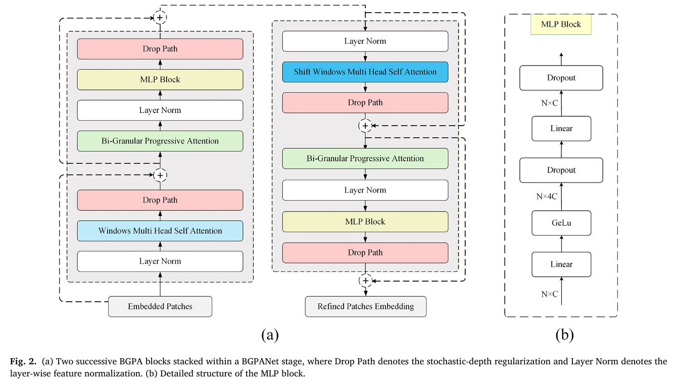
BGPANet uses a Swin-B backbone as its foundation — specifically the Swin Transformer’s hierarchical window attention mechanism, which processes images at progressively lower resolutions and higher semantic abstraction. But the key contribution is what the team inserted at every stage: the BGPA (Bi-Granular Progressive Attention) block, a module that takes the features from each transformer stage and subjects them to a three-branch attention process before passing them forward.
Images are resized to 224×224, partitioned into non-overlapping 4×4 patches (producing a 56×56 grid of 3,136 patches), and fed through the spatial embedding layer. The four subsequent stages contain [2, 2, 18, 2] BGPA blocks respectively. This asymmetric configuration isn’t arbitrary:
- Stages 1 and 2 work on high-resolution feature maps and need only 2 blocks each to capture low-level lesion structure without excessive computation.
- Stage 3 operates at medium resolution where the richest structural information lives, so 18 blocks are stacked to maximize representational depth.
- Stage 4 deals with highly abstract, low-resolution semantics; adding more depth here yields diminishing returns, so 2 blocks suffice before the dense classification head takes over.
The BGPA Block: Three Branches, One Unified Reasoning Process
The BGPA block is the engine of the whole architecture, and it’s worth understanding each of its three branches in detail. Together they implement something close to the human diagnostic process: first establish what matters at the channel level, then locate where it matters in space, then let those two signals talk to each other through local context.
Branch (a): Channel Prior Attention — The Global Semantic Compass
The first branch, the Channel Prior Attention (CPA), answers the question: which feature channels carry the most relevant diagnostic signal? It does this through global average pooling followed by a bottleneck fully-connected module — the same core mechanism as Squeeze-and-Excitation networks, but here repurposed as a semantic prior rather than a standalone attention module.
For an input feature map \\(X \in \mathbb{R}^{H \times W \times C}\\), the global average pooling compresses each channel \\(c\\) into a single scalar descriptor:
This descriptor is then passed through a two-layer bottleneck with a Swish activation in the hidden layer (for gradient stability) and a Sigmoid at the output, producing the channel attention vector \\(\mathbf{g}\\):
The feature map is then reweighted channel-by-channel: \\(X_c(i, j, c) = X(i, j, c) \cdot \mathbf{g}_c\\). This gives you what the authors call the coarse-grained channel feature — a representation where channels associated with lesion-relevant information are amplified and background channels are suppressed, before any spatial reasoning has begun.
Branch (b): Spatial Attention Refinement — Guided by the Channel Prior
With the channel-reweighted features in hand, the second branch asks: where in space do these amplified channels actually fire? This is where BGPANet goes beyond the conventional sequential channel-then-spatial paradigm of CBAM. Instead of computing spatial attention from raw features, it computes it from the channel-reweighted features \\(X_c\\) — meaning the spatial map is already semantically informed by the global prior.
The spatial attention map is built from two statistics at each location \\((i, j)\\): a channel-weighted average and a channel-weighted maximum, concatenated and passed through a 7×7 convolution:
The final fine-grained spatial representation is \\(X_s(i,j,c) = X_c(i,j,c) \cdot M_s(i,j)\\). The result is a feature map where global channel semantics have been baked into the spatial attention computation — the model doesn’t just find interesting locations; it finds locations that are interesting given what it already knows about which features matter.
Branch (c): Cross-Dimensional Collaborative Attention — Local Context with Global Conditioning
The third and most novel branch, the Cross-Dimensional Collaborative Attention (CDCA), performs a conditional local self-attention operation. A 1×1 convolution compresses \\(X_s\\) into a low-dimensional embedding \\(E = \text{Conv}_{1\times1}(X_s)\\) for stable similarity computation. Then, within each non-overlapping window \\(\Omega_w(i,j)\\) of size \\(M \times M\\) (\\(M=4\\) by default), attention weights are computed between all pixel pairs:
The contextual feature is then obtained by a channel-prior-conditioned weighted aggregation over the neighborhood, propagating coarse-grained semantic information into the fine texture representation:
Fusion: The Learnable Convex Combination
The three branch outputs — coarse-grained channel features \\(X_c\\), fine-grained spatial features \\(X_s\\), and cross-dimensional contextual features \\(X_{\text{ctx}}\\) — are fused through a Softmax-parameterized convex combination:
The coefficients are learned during training rather than hand-tuned, allowing the model to adaptively weight each granularity level depending on the specific characteristics of the data distribution. This is a crucial design choice: it means the network can lean more heavily on global semantics for some tasks and more on spatial fine detail for others, without any engineering intervention.
“The proposed architecture introduces a granularity-driven paradigm that progressively transfers coarse-grained semantic priors into fine-grained textures, enabling explicit cross-granularity collaboration across dimensions.” — Liu et al., Expert Systems With Applications 321 (2026) 132169
The Dual-Tailed Loss: Solving Imbalance Without Breaking Training
Even the most sophisticated attention architecture will fail if the training signal doesn’t reach minority classes effectively. Standard Cross-Entropy Loss becomes dominated by the majority class when data is severely skewed — the cumulative gradient from thousands of Nevus samples simply drowns out the signal from a few dozen Dermatofibroma images. Focal Loss was designed to address this: it down-weights easy samples by a factor of \\((1 – \hat{p}_i)^\gamma\\), ensuring hard samples receive proportionally more gradient. But it introduces its own problem: in early training, when the model hasn’t learned anything yet, all samples look hard. The \\((1-\hat{p}_i)^\gamma\\) term amplifies every gradient simultaneously, destabilizing convergence before the model even has a chance to learn basic features.
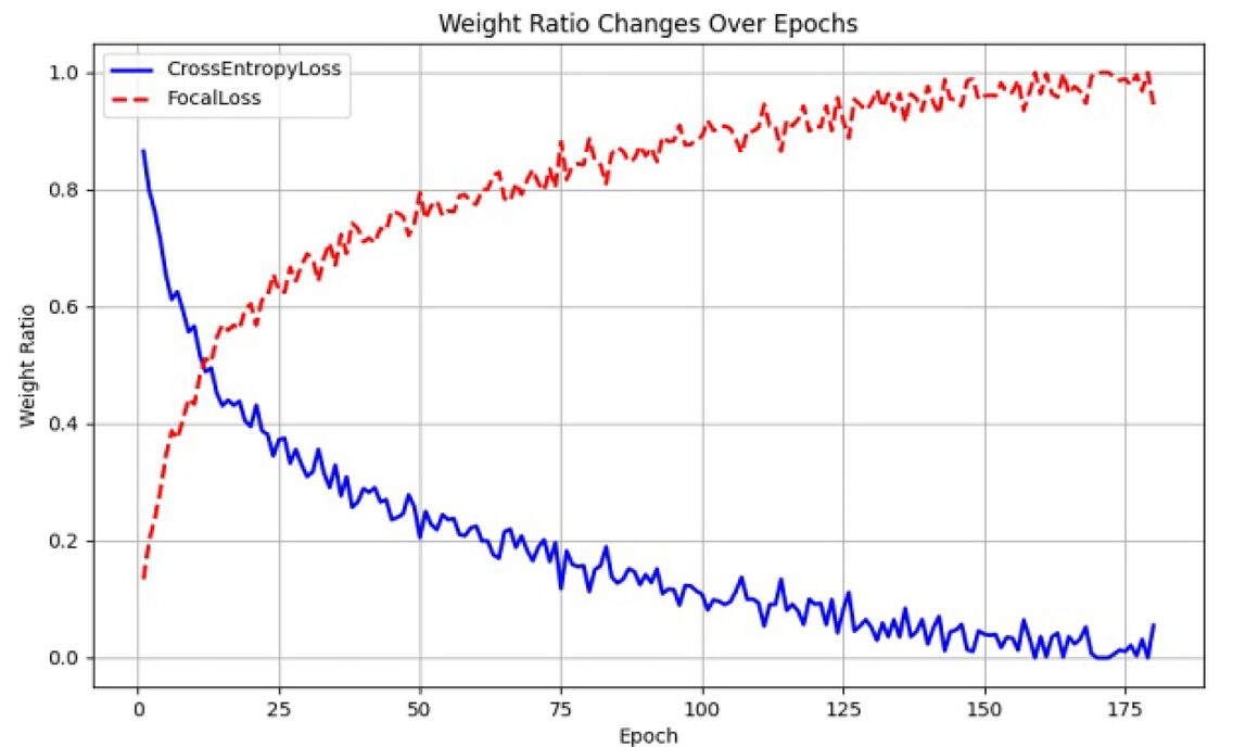
The Dual-Tailed Loss solves this by treating the training schedule itself as a design variable. At step \\(t\\) of a total \\(T\\)-step training run, the loss weights evolve linearly:
When \\(t \approx 0\\), the loss is almost entirely Cross-Entropy: stable gradients guide the model toward learning basic class separability. As training progresses and \\(t \to T\\), Focal Loss takes over, progressively redirecting the gradient budget toward hard-to-classify minority samples. The transition is smooth, automatic, and requires no tuning beyond the single Focal Loss parameter \\(\gamma\\) (set to 2 by default).
Ablation experiments validated this design rigorously. Against five alternative strategies — Cross-Entropy alone, Focal Loss alone, and three fixed-weight combinations (0.4/0.6, 0.5/0.5, 0.6/0.4) plus cosine, exponential, and step-wise schedules — the linear dynamic weighting consistently outperformed everything. Pure Focal Loss actually scored 3.52% lower than the best result, confirming the early-instability hypothesis.
The Dual-Tailed Loss achieves 97.87% accuracy on HAM10000 compared to 96.20% with Cross-Entropy alone and 94.35% with pure Focal Loss. The 3.52-percentage-point gap between BGPANet and the closest static weighting scheme underscores that loss schedule design is as important as architecture design in highly imbalanced medical settings.
Experimental Results: Dominating Both Benchmarks
HAM10000: Seven-Class Multi-Lesion Classification
HAM10000 contains 10,015 dermoscopic images across seven lesion categories, with class sizes ranging from 115 to 6,705 samples — a maximum imbalance ratio of over 58:1. This is a genuine clinical distribution, not a toy dataset, and it punishes models that fail to handle minority classes.
| Model | Accuracy (%) | Precision (%) | Recall (%) | F1-Score (%) | GFLOPs |
|---|---|---|---|---|---|
| ResNet101 | 86.34 | 80.44 | 69.30 | 73.51 | 7.5 |
| VGG16 | 84.87 | 76.86 | 68.14 | 70.81 | 15.5 |
| MobileNetV3-S | 89.46 | 85.01 | 77.84 | 80.87 | 0.6 |
| ViT-Base | 85.33 | 79.12 | 74.67 | 75.91 | 16.8 |
| Swin Transformer | 92.50 | 91.12 | 84.37 | 87.17 | 15.1 |
| HorNet-GF | 92.33 | 88.76 | 85.12 | 86.78 | 15.5 |
| CNN-ViT (Pacal et al., 2025) | 95.01 | 94.70 | 92.11 | 93.34 | — |
| Hybrid ConvNeXt (Aruk et al., 2025) | 94.30 | 93.00 | 89.59 | 91.11 | — |
| BGPANet (ours) | 97.87 | 97.65 | 97.18 | 97.03 | 15.3 |
Table 1: Performance comparison on HAM10000 (five-fold cross-validation). BGPANet surpasses the strongest baseline by 5.37 percentage points in Accuracy and 5.44 points in BMC. All performance differences are statistically significant at p < 0.05 by paired t-test.
ISIC2020: Extreme Binary Imbalance
ISIC2020 presents a different kind of challenge: a binary benign/malignant classification with a 71:1 imbalance ratio. This is a stress test for any loss function claiming to handle skewed distributions. BGPANet achieves 98.43% accuracy — slightly edging out CIFF-Net (98.30%) and MobileNet-V2 (98.20%) — while attaining 99.13% Precision, the highest reported on this dataset.
| Model | Accuracy (%) | Precision (%) | Recall (%) | F1-Score (%) | BMC (%) |
|---|---|---|---|---|---|
| ResNet101 | 92.04 | 93.75 | 90.57 | 90.82 | 56.37 |
| VGG16 | 85.89 | 77.51 | 78.16 | 77.82 | 53.69 |
| Swin Transformer | 90.24 | 90.85 | 81.72 | 79.77 | 57.71 |
| CIFF-Net | 98.30 | — | — | — | — |
| MobileNet-V2 | 98.20 | — | — | — | — |
| DenseNet121 | 95.30 | 94.20 | 93.80 | 95.50 | — |
| BGPANet (ours) | 98.43 | 99.13 | 94.19 | 93.85 | 61.32 |
Table 2: ISIC2020 results. BGPANet achieves the highest Accuracy and Precision, with 99.13% Precision indicating extremely few false positives — critical for clinical screening where unnecessary biopsies carry real patient cost.
Ablation: What Each Component Actually Contributes
The research team ran a thorough ablation study to isolate the contribution of each architectural component. The BGPA block alone (without the Dual-Tailed Loss) pushed HAM10000 accuracy from 92.50% to 96.20%, a 3.7-point gain purely from better feature representation. Adding the Dual-Tailed Loss brings it further to 97.87%. The synergy matters: the attention mechanism finds the right features, and the loss function ensures those features are learned from all classes, not just the majority.
Drilling further into the BGPA block itself, the team evaluated each branch incrementally. CPA alone (channel prior attention only) raised accuracy by 0.95 points. Adding SAR (spatial refinement guided by the channel prior) added another 1.30 points. Adding CDCA (the local contextual self-attention) contributed the final 1.45 points to reach the full BGPA performance. Each branch builds meaningfully on the last — this is cross-granularity collaboration working as intended, not redundant computation.
What BGPANet Gets Right That Others Don’t

What separates BGPANet from the many competing methods that also claim multi-scale or multi-granularity feature learning is the directionality of information flow. Most approaches either concatenate features from different scales or apply channel and spatial attention independently in sequence. BGPANet does something more specific: it uses a global semantic summary as a conditioning signal for both spatial and local contextual attention. The coarse-grained channel prior \\(\mathbf{g}\\) appears in the computation of \\(M_s\\) (spatial attention map) and in the contextual aggregation \\(X_{\text{ctx}}\\) — it’s not just computed and forgotten, it actively shapes the subsequent representations.
This is why the CAM visualizations tell such a clear story. The model isn’t randomly distributing attention across the image; it’s looking at the same regions a trained clinician would — the irregular pigment network, the asymmetric border, the atypical vascular structures — because it has learned to use the channel prior to direct its spatial attention to those high-relevance areas.
The Dual-Tailed Loss, meanwhile, represents a genuinely practical solution to a problem that has no clean theoretical fix. Imbalanced medical datasets are not going away. Collecting balanced datasets in dermatology requires the rarest lesions to appear with the same frequency as common ones — which is simply contrary to reality. A loss function that adapts its focus dynamically across the training curve, starting where the optimizer needs stability and finishing where the model needs to learn rare class boundaries, is far more practical than complex resampling pipelines or ensemble-based balancing strategies.
Complete End-to-End PyTorch Implementation
The following is a complete, self-contained PyTorch implementation of BGPANet, including the BGPA block (all three branches: CPA, SAR, CDCA), the Dual-Tailed Loss with dynamic weight scheduling, and the full model with Swin-B backbone integration. This code is structured for readability and direct training use.
# ═══════════════════════════════════════════════════════════════════════════
# BGPANet: Bi-Granular Progressive Attention for Imbalanced Skin Lesion
# Diagnosis
# Liu, Guo, Yu, et al. · Expert Systems With Applications 321 (2026) 132169
# Complete PyTorch Implementation
# ═══════════════════════════════════════════════════════════════════════════

import torch
import torch.nn as nn
import torch.nn.functional as F
import torchvision.transforms as transforms
from torchvision.models import swin_b, Swin_B_Weights
from torch.utils.data import DataLoader, Dataset
import math
from typing import Optional, List, Tuple


# ─── Section 1: Channel Prior Attention (CPA Branch) ──────────────────────

class ChannelPriorAttention(nn.Module):
    """
    Branch (a) of the BGPA block.
    Computes coarse-grained channel weights via global average pooling
    followed by a bottleneck fully-connected module (Eq. 2 in paper).

    Args:
        channels (int): Number of input feature channels C.
        reduction (int): Bottleneck reduction ratio r (default 16).
    """
    def __init__(self, channels: int, reduction: int = 16):
        super().__init__()
        mid = max(channels // reduction, 8)
        # Two-layer bottleneck: C → C//r → C
        self.fc1 = nn.Linear(channels, mid, bias=True)
        self.fc2 = nn.Linear(mid, channels, bias=True)
        self.sigmoid = nn.Sigmoid()

    def forward(self, x: torch.Tensor) -> Tuple[torch.Tensor, torch.Tensor]:
        """
        Args:
            x: Feature map of shape (B, C, H, W).
        Returns:
            g:   Channel attention vector (B, C, 1, 1) — the 'prior' g.
            x_c: Channel-reweighted features (B, C, H, W).
        """
        B, C, H, W = x.shape

        # Global average pooling: (B, C, H, W) → (B, C)
        z = x.mean(dim=[-2, -1])

        # Bottleneck with Swish activation (Eq. 4 in paper)
        h = F.silu(self.fc1(z))          # Swish ≡ SiLU in PyTorch
        g = self.sigmoid(self.fc2(h))   # (B, C)  — channel weights

        # Reshape for broadcasting: (B, C) → (B, C, 1, 1)
        g = g.view(B, C, 1, 1)

        # Reweight: X_c(i,j,c) = X(i,j,c) · g_c   (Eq. 5)
        x_c = x * g
        return g, x_c


# ─── Section 2: Spatial Attention Refinement (SAR Branch) ─────────────────

class SpatialAttentionRefinement(nn.Module):
    """
    Branch (b) of the BGPA block.
    Constructs a spatial attention map guided by the channel prior g,
    computing channel-weighted average and max statistics per location
    before a 7×7 convolution (Eq. 6–9 in paper).

    Args:
        kernel_size (int): Convolution kernel size for spatial map (default 7).
    """
    def __init__(self, kernel_size: int = 7):
        super().__init__()
        padding = kernel_size // 2
        # Takes concatenated [avg_stat, max_stat] → spatial attention map
        self.conv = nn.Conv2d(2, 1, kernel_size=kernel_size, padding=padding, bias=False)
        self.sigmoid = nn.Sigmoid()

    def forward(self, x_c: torch.Tensor, g: torch.Tensor) -> Tuple[torch.Tensor, torch.Tensor]:
        """
        Args:
            x_c: Channel-reweighted features (B, C, H, W).
            g:   Channel attention weights (B, C, 1, 1).
        Returns:
            M_s: Spatial attention map (B, 1, H, W).
            x_s: Spatially refined features (B, C, H, W).
        """
        # Channel-weighted statistics at each spatial location (Eq. 6, 7)
        # x_c already contains g_c * X_c(i,j,c)
        f_avg = x_c.mean(dim=1, keepdim=True)        # (B, 1, H, W)
        f_max = x_c.max(dim=1, keepdim=True).values  # (B, 1, H, W)

        # Concatenate and apply 7×7 conv → sigmoid (Eq. 8)
        combined = torch.cat([f_avg, f_max], dim=1)   # (B, 2, H, W)
        M_s = self.sigmoid(self.conv(combined))        # (B, 1, H, W)

        # Fine-grained spatial features: X_s = X_c · M_s  (Eq. 9)
        x_s = x_c * M_s
        return M_s, x_s


# ─── Section 3: Cross-Dimensional Collaborative Attention (CDCA Branch) ──

class CrossDimensionalCollaborativeAttention(nn.Module):
    """
    Branch (c) of the BGPA block.
    Performs conditional local self-attention within non-overlapping windows,
    conditioned on the channel prior g (Eq. 10–12 in paper).

    Args:
        channels (int):    Number of feature channels C.
        window_size (int): Local attention window size M (default 4).
    """
    def __init__(self, channels: int, window_size: int = 4):
        super().__init__()
        self.window_size = window_size
        # 1×1 conv for embedding before similarity computation (Eq. 10)
        self.embed = nn.Conv2d(channels, channels, kernel_size=1, bias=False)

    def _window_partition(self, x: torch.Tensor) -> Tuple[torch.Tensor, int, int]:
        """Partition (B, C, H, W) into non-overlapping windows of size M×M."""
        B, C, H, W = x.shape
        M = self.window_size
        # Pad if necessary
        H_pad = (M - H % M) % M
        W_pad = (M - W % M) % M
        if H_pad > 0 or W_pad > 0:
            x = F.pad(x, (0, W_pad, 0, H_pad))
        H_p, W_p = H + H_pad, W + W_pad
        # Reshape to (B * num_windows, C, M, M)
        x = x.view(B, C, H_p // M, M, W_p // M, M)
        x = x.permute(0, 2, 4, 1, 3, 5).contiguous()
        x = x.view(-1, C, M, M)
        return x, H_p, W_p

    def _window_reverse(self, windows: torch.Tensor, B: int, H_p: int, W_p: int) -> torch.Tensor:
        """Reverse window partitioning back to (B, C, H_p, W_p)."""
        M = self.window_size
        C = windows.shape[1]
        windows = windows.view(B, H_p // M, W_p // M, C, M, M)
        windows = windows.permute(0, 3, 1, 4, 2, 5).contiguous()
        return windows.view(B, C, H_p, W_p)

    def forward(self, x_s: torch.Tensor, g: torch.Tensor) -> torch.Tensor:
        """
        Args:
            x_s: Fine-grained spatial features (B, C, H, W).
            g:   Channel prior weights (B, C, 1, 1).
        Returns:
            X_ctx: Cross-dimensional contextual features (B, C, H, W).
        """
        B, C, H, W = x_s.shape
        M = self.window_size

        # 1×1 conv embedding E = Conv_1×1(X_s)  (Eq. 10)
        E = self.embed(x_s)  # (B, C, H, W)

        # Partition into windows
        E_win, H_p, W_p = self._window_partition(E)    # (N_win, C, M, M)
        xs_win, _, _    = self._window_partition(x_s)  # (N_win, C, M, M)
        g_exp = g.expand(B, C, H, W)
        g_win, _, _     = self._window_partition(g_exp)  # (N_win, C, M, M)

        N_win = E_win.shape[0]
        # Flatten spatial: (N_win, C, M, M) → (N_win, M*M, C)
        E_flat  = E_win.view(N_win, C, -1).permute(0, 2, 1)   # (N_win, M², C)
        xs_flat = xs_win.view(N_win, C, -1).permute(0, 2, 1)   # (N_win, M², C)
        g_flat  = g_win.view(N_win, C, -1).permute(0, 2, 1)    # (N_win, M², C)

        # Local self-attention: A = softmax(E @ E^T / scale) (Eq. 11)
        scale = math.sqrt(C)
        A = torch.bmm(E_flat, E_flat.transpose(1, 2)) / scale  # (N_win, M², M²)
        A = F.softmax(A, dim=-1)

        # Channel-prior conditioned aggregation  (Eq. 12)
        # g_flat * xs_flat = channel-conditioned values
        cond_vals = g_flat * xs_flat  # (N_win, M², C)
        ctx_delta = torch.bmm(A, cond_vals)  # (N_win, M², C)

        # Residual: X_ctx = X_s + aggregated context
        x_ctx_flat = xs_flat + ctx_delta  # (N_win, M², C)

        # Unflatten and reverse window partition
        x_ctx_win = x_ctx_flat.permute(0, 2, 1).view(N_win, C, M, M)
        x_ctx = self._window_reverse(x_ctx_win, B, H_p, W_p)  # (B, C, H_p, W_p)
        return x_ctx[:, :, :H, :W]  # remove any padding


# ─── Section 4: Full BGPA Block ────────────────────────────────────────────

class BGPABlock(nn.Module):
    """
    Bi-Granular Progressive Attention Block.
    Integrates CPA → SAR → CDCA branches with a learnable convex
    combination (α, β, γ) to fuse multi-granularity representations
    (Eq. 13 in paper).

    Args:
        channels (int):    Feature channel count C.
        reduction (int):   CPA bottleneck reduction ratio (default 16).
        window_size (int): CDCA local attention window M (default 4).
    """
    def __init__(self, channels: int, reduction: int = 16, window_size: int = 4):
        super().__init__()
        self.cpa  = ChannelPriorAttention(channels, reduction)
        self.sar  = SpatialAttentionRefinement()
        self.cdca = CrossDimensionalCollaborativeAttention(channels, window_size)

        # Learnable convex combination weights (α, β, γ) via softmax
        # Initialized equally; updated during training
        self.mix_logits = nn.Parameter(torch.zeros(3))

    def forward(self, x: torch.Tensor) -> torch.Tensor:
        """
        Args:
            x: Input features (B, C, H, W).
        Returns:
            Y: Fused bi-granular features (B, C, H, W).
        """
        # Branch (a): Channel Prior Attention
        g, x_c = self.cpa(x)           # g: (B,C,1,1), x_c: (B,C,H,W)

        # Branch (b): Spatial Attention Refinement
        M_s, x_s = self.sar(x_c, g)   # M_s: (B,1,H,W), x_s: (B,C,H,W)

        # Branch (c): Cross-Dimensional Collaborative Attention
        x_ctx = self.cdca(x_s, g)     # x_ctx: (B,C,H,W)

        # Learnable convex combination: α·X_c + β·X_s + γ·X_ctx  (Eq. 13)
        weights = F.softmax(self.mix_logits, dim=0)  # ensures α+β+γ=1, all >0
        alpha, beta, gamma = weights[0], weights[1], weights[2]

        Y = alpha * x_c + beta * x_s + gamma * x_ctx
        return Y


# ─── Section 5: Dual-Tailed Loss Function ────────────────────────────────

class DualTailedLoss(nn.Module):
    """
    Dynamic weighted combination of Cross-Entropy and Focal Loss.
    α(t) = 1 - t/T  (Cross-Entropy weight, starts high, decays)
    β(t) = t/T       (Focal Loss weight, starts zero, grows)
    (Eq. 18–20 in paper)

    Args:
        num_classes (int): Number of output classes.
        gamma (float):     Focal loss focusing parameter γ (default 2.0).
        total_steps (int): Total training steps T.
    """
    def __init__(self, num_classes: int, gamma: float = 2.0, total_steps: int = 10000):
        super().__init__()
        self.num_classes = num_classes
        self.gamma = gamma
        self.total_steps = total_steps
        self.current_step = 0

    def step(self):
        """Call after each optimizer.step() to advance the schedule."""
        self.current_step = min(self.current_step + 1, self.total_steps)

    def _cross_entropy(self, logits: torch.Tensor, targets: torch.Tensor) -> torch.Tensor:
        """Standard multi-class cross-entropy loss (Eq. 14)."""
        return F.cross_entropy(logits, targets)

    def _focal_loss(self, logits: torch.Tensor, targets: torch.Tensor) -> torch.Tensor:
        """
        Multi-class focal loss (Eq. 15).
        Reduces weight for well-classified samples via (1 - p_hat)^gamma.
        """
        log_probs = F.log_softmax(logits, dim=1)
        probs     = torch.exp(log_probs)

        # Gather the probability and log-probability for the true class
        batch_size = logits.size(0)
        p_hat = probs[torch.arange(batch_size), targets]      # (B,)
        log_p = log_probs[torch.arange(batch_size), targets]  # (B,)

        # Focal weight: (1 - p_hat)^gamma
        focal_weight = (1.0 - p_hat) ** self.gamma

        loss = -(focal_weight * log_p).mean()
        return loss

    def forward(self, logits: torch.Tensor, targets: torch.Tensor) -> torch.Tensor:
        """
        Args:
            logits:  Model output (B, num_classes).
            targets: Ground-truth class indices (B,).
        Returns:
            Scalar loss value.
        """
        t = self.current_step
        T = self.total_steps

        # Dynamic weights: α(t) = 1 - t/T, β(t) = t/T
        alpha_t = 1.0 - (t / T)
        beta_t  = t / T

        L_ce    = self._cross_entropy(logits, targets)
        L_focal = self._focal_loss(logits, targets)

        return alpha_t * L_ce + beta_t * L_focal


# ─── Section 6: BGPANet Model ─────────────────────────────────────────────

class BGPANet(nn.Module):
    """
    Bi-Granular Progressive Attention Network for skin lesion classification.

    Architecture:
      - Swin-B backbone (pretrained on ImageNet)
      - BGPA block inserted after each Swin stage's feature output
      - Dense classification head mapping to num_classes

    The Swin-B stages produce feature maps of channels:
        Stage 0: 128-ch (H/4  × W/4)
        Stage 1: 256-ch (H/8  × W/8)
        Stage 2: 512-ch (H/16 × W/16)
        Stage 3: 1024-ch (H/32 × W/32)

    BGPA blocks are applied at each stage. Final classification uses
    the last (Stage 3) features after global average pooling.

    Args:
        num_classes (int):  Number of skin lesion categories (7 for HAM10000,
                            2 for ISIC2020).
        reduction (int):    CPA bottleneck reduction ratio (default 16).
        window_size (int):  CDCA window size (default 4).
        pretrained (bool):  Use ImageNet pretrained Swin-B weights.
    """
    def __init__(self,
                 num_classes: int = 7,
                 reduction: int = 16,
                 window_size: int = 4,
                 pretrained: bool = True):
        super().__init__()

        # Load Swin-B backbone
        weights = Swin_B_Weights.DEFAULT if pretrained else None
        swin = swin_b(weights=weights)

        # Extract Swin stages. torchvision's swin_b .features contains:
        # [PatchEmbed, stage0, merge0, stage1, merge1, stage2, merge2, stage3, norm]
        self.patch_embed = swin.features[0]  # Patch partition + embedding

        # Stages and patch merging layers
        self.stage0 = swin.features[1]   # 128-ch, ×2 blocks
        self.merge0 = swin.features[2]   # PatchMerging: 128→256
        self.stage1 = swin.features[3]   # 256-ch, ×2 blocks
        self.merge1 = swin.features[4]   # PatchMerging: 256→512
        self.stage2 = swin.features[5]   # 512-ch, ×18 blocks
        self.merge2 = swin.features[6]   # PatchMerging: 512→1024
        self.stage3 = swin.features[7]   # 1024-ch, ×2 blocks
        self.norm   = swin.features[8]   # LayerNorm

        # BGPA blocks for each stage
        self.bgpa0 = BGPABlock(128,  reduction, window_size)
        self.bgpa1 = BGPABlock(256,  reduction, window_size)
        self.bgpa2 = BGPABlock(512,  reduction, window_size)
        self.bgpa3 = BGPABlock(1024, reduction, window_size)

        # Dense classification head
        self.classifier = nn.Linear(1024, num_classes)

    def _seq_to_spatial(self, x: torch.Tensor) -> torch.Tensor:
        """Convert (B, H*W, C) → (B, C, H, W) for BGPA processing."""
        B, L, C = x.shape
        H = W = int(math.isqrt(L))
        x = x.permute(0, 2, 1).view(B, C, H, W)
        return x

    def _spatial_to_seq(self, x: torch.Tensor) -> torch.Tensor:
        """Convert (B, C, H, W) → (B, H*W, C) for Swin merging layers."""
        B, C, H, W = x.shape
        x = x.view(B, C, H * W).permute(0, 2, 1)
        return x

    def forward(self, x: torch.Tensor) -> torch.Tensor:
        """
        Forward pass for BGPANet.

        Args:
            x: Input dermoscopic images (B, 3, 224, 224).
        Returns:
            logits: Class scores (B, num_classes).
        """
        # ── Patch Embedding ──────────────────────────────────────────────
        x = self.patch_embed(x)  # (B, 56*56, 128) — sequence format

        # ── Stage 0 (128-ch) + BGPA ──────────────────────────────────────
        x = self.stage0(x)                  # (B, 56²,  128)
        sp = self._seq_to_spatial(x)        # (B, 128,  56, 56)
        sp = self.bgpa0(sp)                 # BGPA: coarse→fine pass
        x  = self._spatial_to_seq(sp)       # (B, 56²,  128)
        x  = self.merge0(x)                 # (B, 28²,  256)

        # ── Stage 1 (256-ch) + BGPA ──────────────────────────────────────
        x = self.stage1(x)
        sp = self._seq_to_spatial(x)        # (B, 256, 28, 28)
        sp = self.bgpa1(sp)
        x  = self._spatial_to_seq(sp)
        x  = self.merge1(x)                 # (B, 14², 512)

        # ── Stage 2 (512-ch, ×18 blocks) + BGPA ──────────────────────────
        x = self.stage2(x)
        sp = self._seq_to_spatial(x)        # (B, 512, 14, 14)
        sp = self.bgpa2(sp)
        x  = self._spatial_to_seq(sp)
        x  = self.merge2(x)                 # (B, 7², 1024)

        # ── Stage 3 (1024-ch) + BGPA ─────────────────────────────────────
        x = self.stage3(x)
        sp = self._seq_to_spatial(x)        # (B, 1024, 7, 7)
        sp = self.bgpa3(sp)
        x  = self._spatial_to_seq(sp)

        # ── LayerNorm + Global Average Pool ──────────────────────────────
        x = self.norm(x)                    # (B, 49, 1024)
        x = x.mean(dim=1)                  # (B, 1024)

        # ── Dense Classification Head ─────────────────────────────────────
        logits = self.classifier(x)         # (B, num_classes)
        return logits


# ─── Section 7: Training Pipeline ────────────────────────────────────────

def get_transforms(train: bool = True) -> transforms.Compose:
    """
    Data transforms matching Section 4.3 of the paper.
    Training: augmentation (flip, brightness, hue, saturation, contrast) + normalize.
    Validation/Test: resize + normalize only.
    """
    normalize = transforms.Normalize(
        mean=[0.485, 0.456, 0.406],
        std=[0.229, 0.224, 0.225]
    )
    if train:
        return transforms.Compose([
            transforms.Resize((224, 224)),
            transforms.RandomHorizontalFlip(p=0.5),
            transforms.RandomVerticalFlip(p=0.5),
            transforms.ColorJitter(
                brightness=0.2,    # [0.8, 1.2]
                contrast=0.2,      # [0.8, 1.2]
                saturation=0.2,    # [0.8, 1.2]
                hue=0.1            # [-0.1, 0.1]
            ),
            transforms.ToTensor(),
            normalize
        ])
    else:
        return transforms.Compose([
            transforms.Resize((224, 224)),
            transforms.ToTensor(),
            normalize
        ])


def train_bgpanet(
    num_classes: int,
    train_loader: DataLoader,
    val_loader: DataLoader,
    num_epochs: int = 180,
    device: str = "cuda"
) -> BGPANet:
    """
    Full training loop for BGPANet following paper hyperparameters (Table 2):
      - AdamW optimizer, lr=1e-4, weight_decay=0.05
      - Cosine annealing with 5-epoch warm-up
      - Dual-Tailed Loss with linear dynamic weighting
      - Early stopping on validation loss
      - Total epochs: 180

    Args:
        num_classes:   7 (HAM10000) or 2 (ISIC2020).
        train_loader:  Training DataLoader.
        val_loader:    Validation DataLoader.
        num_epochs:    Maximum training epochs (default 180).
        device:        'cuda' or 'cpu'.

    Returns:
        Trained BGPANet model (best checkpoint).
    """
    device = torch.device(device if torch.cuda.is_available() else "cpu")
    print(f"Training on: {device}")

    # Model
    model = BGPANet(num_classes=num_classes, pretrained=True).to(device)

    # Compute total training steps for Dual-Tailed Loss schedule
    total_steps = num_epochs * len(train_loader)

    # Loss and optimizer
    criterion = DualTailedLoss(
        num_classes=num_classes,
        gamma=2.0,
        total_steps=total_steps
    )
    optimizer = torch.optim.AdamW(
        model.parameters(),
        lr=1e-4,
        weight_decay=0.05
    )

    # Cosine annealing LR scheduler
    scheduler = torch.optim.lr_scheduler.CosineAnnealingLR(
        optimizer,
        T_max=num_epochs,
        eta_min=1e-6
    )

    # Warm-up: linearly scale LR for first 5 epochs
    warmup_epochs = 5
    warmup_scheduler = torch.optim.lr_scheduler.LinearLR(
        optimizer, start_factor=0.01, end_factor=1.0, total_iters=warmup_epochs
    )

    best_val_loss = float("inf")
    best_val_acc  = 0.0
    patience      = 20
    no_improve    = 0
    best_state    = None

    for epoch in range(1, num_epochs + 1):
        # ── Training Phase ───────────────────────────────────────────
        model.train()
        total_loss = correct = total = 0

        for images, labels in train_loader:
            images = images.to(device)
            labels = labels.to(device)

            optimizer.zero_grad()
            logits = model(images)
            loss   = criterion(logits, labels)
            loss.backward()
            optimizer.step()
            criterion.step()  # advance Dual-Tailed Loss schedule

            total_loss += loss.item() * images.size(0)
            preds = logits.argmax(dim=1)
            correct += (preds == labels).sum().item()
            total += images.size(0)

        train_acc  = correct / total
        train_loss = total_loss / total

        # ── Validation Phase ─────────────────────────────────────────
        model.eval()
        val_loss = val_correct = val_total = 0

        with torch.no_grad():
            for images, labels in val_loader:
                images = images.to(device)
                labels = labels.to(device)
                logits = model(images)
                loss   = criterion(logits, labels)
                val_loss += loss.item() * images.size(0)
                preds = logits.argmax(dim=1)
                val_correct += (preds == labels).sum().item()
                val_total   += images.size(0)

        val_acc  = val_correct / val_total
        val_loss /= val_total

        # LR scheduling
        if epoch <= warmup_epochs:
            warmup_scheduler.step()
        else:
            scheduler.step()

        print(f"Epoch [{epoch:3d}/{num_epochs}] "
              f"Train Loss: {train_loss:.4f} Acc: {train_acc:.4f} | "
              f"Val Loss: {val_loss:.4f} Acc: {val_acc:.4f}")

        # Early stopping on best validation accuracy
        if val_acc > best_val_acc:
            best_val_acc = val_acc
            best_state   = {k: v.cpu().clone() for k, v in model.state_dict().items()}
            no_improve   = 0
        else:
            no_improve += 1
            if no_improve >= patience:
                print(f"Early stopping triggered at epoch {epoch}.")
                break

    # Restore best checkpoint
    model.load_state_dict(best_state)
    print(f"\nTraining complete. Best Val Accuracy: {best_val_acc:.4f}")
    return model


# ─── Section 8: Quick Sanity Check ────────────────────────────────────────

if __name__ == "__main__":
    print("=" * 65)
    print("BGPANet — Bi-Granular Progressive Attention Network")
    print("Liu et al. · Expert Systems With Applications 321 (2026)")
    print("=" * 65)

    device = "cuda" if torch.cuda.is_available() else "cpu"

    # ── 1. Model instantiation ────────────────────────────────────────
    print("\n[1] Building BGPANet for HAM10000 (7-class)...")
    model = BGPANet(num_classes=7, pretrained=False).to(device)

    total_params = sum(p.numel() for p in model.parameters())
    print(f"    Total parameters: {total_params / 1e6:.1f}M")

    # ── 2. Forward pass ───────────────────────────────────────────────
    print("\n[2] Running forward pass on synthetic batch...")
    dummy_input  = torch.randn(4, 3, 224, 224).to(device)  # batch of 4
    dummy_labels = torch.randint(0, 7, (4,)).to(device)

    with torch.no_grad():
        logits = model(dummy_input)
    print(f"    Input shape:  {dummy_input.shape}")
    print(f"    Output shape: {logits.shape}")
    print(f"    ✓ Forward pass successful")

    # ── 3. Dual-Tailed Loss ────────────────────────────────────────────
    print("\n[3] Testing Dual-Tailed Loss schedule...")
    criterion = DualTailedLoss(num_classes=7, gamma=2.0, total_steps=100)

    losses_at_steps = []
    for step in [0, 25, 50, 75, 100]:
        criterion.current_step = step
        alpha_t = 1.0 - step / 100
        beta_t  = step / 100
        losses_at_steps.append((step, alpha_t, beta_t))
        print(f"    Step {step:3d}/100 → α(CE)={alpha_t:.2f}, β(Focal)={beta_t:.2f}")

    # Reset and compute actual loss on dummy batch
    criterion.current_step = 50
    loss_val = criterion(logits, dummy_labels)
    print(f"    ✓ Loss at step 50: {loss_val.item():.4f}")

    # ── 4. BGPA Block ablation check ──────────────────────────────────
    print("\n[4] Individual branch outputs from BGPA block...")
    bgpa = BGPABlock(channels=128, reduction=16, window_size=4).to(device)
    feat = torch.randn(2, 128, 56, 56).to(device)  # Stage-0 feature map
    out  = bgpa(feat)
    print(f"    Input:  {feat.shape}")
    print(f"    Output: {out.shape}")
    alpha, beta, gamma = F.softmax(bgpa.mix_logits, dim=0).detach()
    print(f"    Fusion weights — α:{alpha:.3f}  β:{beta:.3f}  γ:{gamma:.3f}")
    print(f"    ✓ BGPA block verified")

    print("\n" + "=" * 65)
    print("All components verified. Ready for training on HAM10000/ISIC2020.")
    print("=" * 65)
Access the Paper and Dataset Resources
The full BGPANet framework is published in Expert Systems With Applications. Both datasets used in this study are publicly available. Contact the first author for model weights.
Liu, M., Guo, R., Yu, X., Yu, Z., Xiao, Z., & Jiang, X. (2026). BGPANet: Bi-Granular progressive attention for imbalanced skin lesion diagnosis. Expert Systems With Applications, 321, 132169. https://doi.org/10.1016/j.eswa.2026.132169
This article is an independent editorial analysis of peer-reviewed research published in Expert Systems With Applications. The PyTorch implementation is provided for educational and research purposes to illustrate the architectural principles described in the paper. The code is a faithful interpretation of the published method but has not been validated by the original authors. For the official implementation, contact the corresponding author at liuming@ccut.edu.cn. Always refer to the original publication for authoritative algorithmic details.