Understanding Brain Surface Registration and Its Clinical Significance
The human brain’s cortex is one of nature’s most complex structures, characterized by intricate folds and highly variable topography across individuals. This anatomical complexity presents a fundamental challenge for neuroscientists and clinical researchers: how can we reliably compare brain structures and functions across different people when each brain is uniquely configured?
Cortical surface registration—the process of aligning brain surfaces from different individuals to a common reference space—is the answer to this challenge. By mapping data to a standardized anatomical space, researchers can conduct comparative analyses that would otherwise be impossible. This capability underpins critical applications including cortical morphometry studies, functional connectivity research, neurodevelopmental investigations, and neurosurgical planning.
However, traditional registration methods have struggled with a fundamental problem: balancing alignment accuracy against computational efficiency while maintaining biologically plausible deformations. Enter GeoMorph, a novel deep learning framework that fundamentally transforms how we approach this problem.
The Challenge of Brain Surface Alignment
Why Traditional Methods Fall Short
Conventional cortical registration relies primarily on univariate features—single measurements like sulcal depth or cortical curvature. While these approaches provide reasonable alignment for gross anatomical features, they fail to capture the nuanced organization of functional brain areas. Brain folds don’t perfectly localize all cortical functions, meaning that alignment based purely on folding patterns misses crucial information about where specific brain functions are actually located.
Key limitations of classical approaches include:
- Computational intensity: Methods like Multimodal Surface Matching (MSM) require hours of processing time per brain due to complex combinatorial optimization problems
- Inflexibility: Classical frameworks struggle to incorporate multiple data types simultaneously, limiting alignment accuracy when dealing with diverse brain features
- Feature limitation: Reliance on folding patterns alone misses important functional organization that doesn’t correlate with surface convolutions
- Noise sensitivity: Traditional algorithms can struggle with noisy functional data, such as resting-state fMRI and myelin maps
The Multimodal Registration Revolution
Modern neuroscience recognizes that optimal brain alignment requires multimodal information—combining structural features (like T1-weighted to T2-weighted intensity ratios indicating myelin content) with functional data (resting-state networks and task-based fMRI activations). This multimodal approach dramatically improves the spatial localization of functional areas across individuals, enabling more precise group-level neuroscientific findings.
Yet multimodal registration introduces new challenges: each data type has unique noise characteristics and sparsity patterns, requiring sophisticated feature extraction before alignment can proceed effectively.
Introducing GeoMorph: Architecture and Innovation
Core Architectural Components
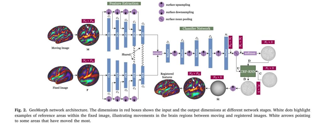
GeoMorph represents a paradigm shift in brain surface registration by combining three innovative components: independent feature extraction, deep-discrete registration, and conditional random field regularization.
The framework operates on spherical representations of cortical surfaces—an elegant mathematical choice that better preserves geodesic distances between brain points than other parameterizations. The registration process involves learning optimal displacements for a set of control points distributed across this spherical surface, such that features on a moving brain surface optimally align with those on a fixed reference brain.
The three-stage processing pipeline consists of:
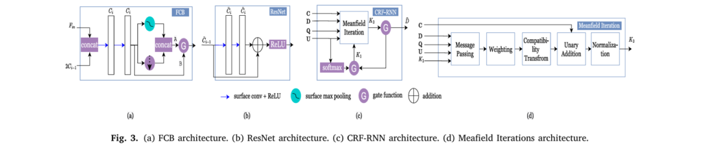
- Feature Extraction Network: Independently processes moving and fixed cortical features through separate pathways to learn low-dimensional representations capturing essential cortical characteristics. This is particularly crucial for multimodal registration where different feature types have distinct noise distributions.
- Classifier Network: Transforms extracted features through ResNet-inspired blocks, outputting probability distributions over potential displacement labels for each control point.
- CRF-RNN Regularization: Implements a deep conditional random field using recurrent neural network iterations to enforce smoothness by encouraging neighboring control points to deform similarly.
Mathematical Framework
The core optimization objective combines a similarity metric with smoothness regularization:
$$\hat{\boldsymbol{\theta}} = \arg\min_{\boldsymbol{\theta}} \mathcal{L}{sim}(\boldsymbol{\Phi}{\boldsymbol{\theta}}; \mathbf{F}, \mathbf{M}) + \mathcal{L}{sm}(\boldsymbol{\Phi}{\boldsymbol{\theta}})$$where the similarity loss combines mean-squared error with cross-correlation:
$$\mathcal{L}{sim} = \frac{1}{N_d}\sum{i=1}^{N_d}\left(|\mathbf{F}_{\mathbf{v}i} – \bar{\mathbf{M}}{\mathbf{v}i}|2^2 – \frac{\text{cov}(\mathbf{F}{\mathbf{v}i}, \bar{\mathbf{M}}{\mathbf{v}i})}{\sigma{\mathbf{F}} \sigma{\bar{\mathbf{M}}}}\right)$$The smoothness penalty applies diffusion regularization on deformation gradients across the spherical surface.
Geometric Convolutions on Spherical Surfaces
A critical innovation in GeoMorph is its use of MoNet-style geometric convolutions, which operate directly on non-Euclidean spherical surface data. These convolutions employ Gaussian mixture models to define learnable spatial interactions:
$$w_j(\mathbf{u}) = \exp\left(-\frac{1}{2}(\mathbf{u} – \boldsymbol{\mu}_j)^T \boldsymbol{\Sigma}_j^{-1}(\mathbf{u} – \boldsymbol{\mu}_j)\right)$$
This approach provides empirical robustness to rotational transformations—a critical property when processing brain data where orientation can vary arbitrarily across the training dataset.
Performance Advantages Over Existing Methods
Computational Efficiency Breakthrough
The performance comparisons are striking. GeoMorph achieves registration in approximately 2.6 seconds on GPU compared to 1 hour for classical methods like MSM Strain, representing a 1,400x acceleration in processing time. This dramatic efficiency gain stems from the deep learning approach’s ability to leverage modern hardware and avoid the combinatorial optimization problems that plague discrete classical methods.
| Method | Cross-Correlation | Areal Distortion (Mean) | GPU Time | CPU Time |
|---|---|---|---|---|
| Freesurfer | 0.75 | 0.34 | – | 30 min |
| MSM Strain | 0.880 | 0.27 | – | 1 hour |
| Spherical Demons | 0.875 | 0.18 | – | 1 min |
| S3Reg | 0.875 | 0.26 | 8.0 s | 8.8 s |
| GeoMorph | 0.875 | 0.19 | 2.6 s | 8.3 s |
Alignment Quality and Smoothness
While achieving dramatic speedups, GeoMorph maintains competitive alignment quality with classical methods. For univariate alignment using sulcal depth features, GeoMorph achieves cross-correlation of 0.875—equivalent to Spherical Demons and S3Reg, and nearly matching MSM Strain’s 0.880.
More impressively, GeoMorph produces significantly smoother deformations than competing deep learning methods. Its mean areal distortion of 0.19 substantially outperforms S3Reg’s 0.26 and MSM Pair’s 0.41, indicating that the learned deformations preserve cortical geometry more faithfully.
Multimodal Registration Excellence
For the more challenging multimodal alignment task incorporating T1w/T2w myelin maps and resting-state fMRI networks, GeoMorph achieves 0.975 cross-correlation on myelin data—exceeding MSMAll’s 0.945 on the Human Connectome Project dataset. This improvement reflects GeoMorph’s superior ability to handle the noise and sparsity inherent in functional brain data.
When tested on independently acquired task fMRI data, GeoMorphAll produces sharper and clearer group-level activation maps compared to MSMAll, validating that improved anatomical alignment truly enhances downstream neuroscientific analyses.
Generalization Across Different Datasets
A critical validation emerged from cross-dataset generalization testing. GeoMorph was trained exclusively on the Human Connectome Project (HCP) dataset, then evaluated on the UK Biobank dataset—acquired with substantially different scanning parameters, at different ages (older adults), and with noisier data quality.
Generalization results demonstrate remarkable robustness:
- Myelin cross-correlation decreased only marginally from 0.975 to 0.955
- Areal distortion measures remained comparable
- The model maintained functional registration quality across datasets
This generalization capability suggests GeoMorph can be deployed in diverse clinical and research settings without dataset-specific retraining—a substantial practical advantage.
Technical Innovations: Why GeoMorph Succeeds
Independent Feature Extraction for Multimodal Data
Most existing deep learning registration methods use unified feature extraction pipelines. GeoMorph innovates by maintaining separate feature extraction pathways for moving and fixed images until high-level representation layers. This architecture recognizes that different feature types (structural versus functional, high signal-to-noise versus inherently noisy) may require distinct low-level processing before abstract feature representations can meaningfully correspond.
Weight sharing is applied selectively—only the final two feature extraction blocks share weights, promoting consistency in high-level feature extraction where representations become modality-agnostic, while earlier layers retain independence to capture diverse patterns.
Deep Conditional Random Fields for Anatomically Plausible Deformations
Rather than explicitly enforcing diffeomorphisms (topology-preserving transformations) through constraining parametrization, GeoMorph uses implicit regularization via deep CRFs implemented as recurrent neural networks. The CRF energy function optimizes:
$$E = \sum_i Q(\mathbf{c}i, \mathbf{l}i) + \sum{i \neq j} \varphi(\mathbf{l}{\mathbf{c}i}, \mathbf{l}{\mathbf{c}_j})$$This approach encourages smooth deformations through learned pairwise penalties that capture spatial relationships between control points. Notably, GeoMorph achieves anatomically plausible deformations without explicit diffeomorphic constraints—all observed deformations prove diffeomorphic naturally through regularization strength.
Practical Implication: Breaking Strict Diffeomorphic Constraints
This finding has profound implications. While diffeomorphisms have long been considered necessary for cortical registration, emerging neuroscience evidence shows that cortical topography sometimes changes non-diffeomorphically across individuals (approximately 10% of subjects in critical functional areas). GeoMorph’s regularization approach provides a pathway to explore relaxing this constraint in future work, potentially improving alignment for these exceptional cases.
Real-World Applications and Impact
Clinical Neurosurgery Planning
The 1,400x computational speedup enables practical applications previously infeasible with classical methods. Neurosurgeons could receive real-time pre-operative planning information based on anatomically normalized functional brain maps—critical for preserving eloquent cortex during tumor resection.
Large-Scale Population Neuroscience
With UK Biobank containing 50,000+ brain scans and emerging longitudinal studies acquiring thousands of images, the computational efficiency becomes transformative. Researchers can now create precise population-average templates conditioned on demographic variables or clinical phenotypes, enabling discovery of cortical organizational principles across populations.
Functional Connectivity and Network Analysis
More accurate alignment directly improves group-level functional connectivity analysis. The sharper group-level resting-state maps demonstrated in GeoMorph validation enable more sensitive detection of connectivity differences between clinical populations.
Limitations and Future Research Directions
GeoMorph’s authors identify several important areas for future development:
Memory constraints limit the control point grid resolution to icosphere level 4. Future work could explore more memory-efficient architectures enabling higher-resolution control grids for even more precise alignment.
Rotational equivariance remains partially addressed. While MoNet provides empirical robustness, theoretically grounded rotationally equivariant convolutions like SE(3)-equivariant networks could improve feature learning, though at substantial computational cost.
Learnable mechanical regularization replacing the CRF with physically-informed penalties that incorporate brain tissue properties could produce even more biologically faithful deformations.
Attention mechanisms through surface vision transformers could enable more precise feature alignment through context-aware processing of complex cortical variations.
Conclusion: A New Standard for Brain Surface Registration
GeoMorph represents a watershed moment in neuroimaging methodology. By combining geometric deep learning with insights from classical registration frameworks, it achieves previously unattainable combinations of speed, accuracy, smoothness, and generalization capability.
The framework’s ability to handle multimodal data—simultaneously leveraging structural and functional information—aligns with modern neuroscience’s recognition that brain organization transcends simple folding patterns. The 1,400x computational acceleration opens applications that were computationally infeasible mere years ago.
Most significantly, GeoMorph demonstrates that learning-based approaches need not sacrifice the anatomical plausibility that has defined successful registration methods. Instead, through careful architectural design and regularization, we can achieve the efficiency benefits of deep learning while maintaining the biological fidelity that neuroscientists demand.
As neuroimaging studies grow to unprecedented scales and clinical applications demand real-time processing, GeoMorph provides the tools for a new generation of brain-mapping research. The framework is openly available on GitHub, enabling rapid adoption and inspiring future innovations in geometric deep learning for medical imaging.
For neuroscience researchers, computational biologists, and neuroimaging engineers, GeoMorph offers a powerful, practical tool that fundamentally advances our ability to understand and map the human brain. Explore the code, apply it to your research questions, and join the emerging community working at the intersection of deep learning and neuroanatomy.
The full paper is available here. (https://www.sciencedirect.com/science/article/pii/S1361841525003676)
Below is a comprehensive end-to-end python implementation of GeoMorph with 9 major components:
"""
GeoMorph: Unsupervised Multimodal Surface Registration with Geometric Deep Learning
Complete implementation of the cortical surface registration framework.
"""

import torch
import torch.nn as nn
import torch.nn.functional as F
from torch_geometric.nn import MoNetConv
from torch_geometric.data import Data
import numpy as np
from typing import Tuple, Optional, List
import math


# ============================================================================
# 1. GEOMETRIC CONVOLUTION LAYERS
# ============================================================================

class MoNetConvBlock(nn.Module):
    """
    Mixture of Experts convolution block using Gaussian mixture models.
    Provides robustness to rotational transformations on spherical surfaces.
    """
    def __init__(self, in_channels: int, out_channels: int, num_kernels: int = 10):
        super().__init__()
        self.in_channels = in_channels
        self.out_channels = out_channels
        self.num_kernels = num_kernels

        # Learnable Gaussian kernel parameters
        self.mu = nn.Parameter(torch.randn(num_kernels, 3))
        self.sigma = nn.ParameterList([
            nn.Parameter(torch.eye(3)) for _ in range(num_kernels)
        ])

        # Output filters for each kernel
        self.kernel_weights = nn.Linear(num_kernels, out_channels)
        self.bias = nn.Parameter(torch.zeros(out_channels))

    def forward(self, x: torch.Tensor, edge_index: torch.Tensor,
                pseudo_coords: torch.Tensor) -> torch.Tensor:
        """
        Args:
            x: Node features [num_nodes, in_channels]
            edge_index: Edge connectivity [2, num_edges]
            pseudo_coords: Pseudo-coordinates [num_edges, 3]
        """
        # Compute Gaussian basis functions
        diff = pseudo_coords.unsqueeze(1) - self.mu.unsqueeze(0)  # [num_edges, num_kernels, 3]

        weights = []
        for k in range(self.num_kernels):
            sigma_inv = torch.inverse(self.sigma[k])
            mahal = torch.sum(diff[:, k:k+1, :] @ sigma_inv * diff[:, k:k+1, :], dim=2)
            w_k = torch.exp(-0.5 * mahal)
            weights.append(w_k)

        weights = torch.cat(weights, dim=1)  # [num_edges, num_kernels]

        # Aggregate neighbor features with Gaussian weighting
        src, dst = edge_index
        weighted_features = x[src] * weights.unsqueeze(2)  # [num_edges, num_kernels, in_channels]

        # Sum aggregation for each node
        aggregated = torch.zeros(x.size(0), self.num_kernels, self.in_channels,
                                device=x.device, dtype=x.dtype)
        aggregated = aggregated.scatter_add_(0, dst.unsqueeze(1).unsqueeze(2).expand(-1, self.num_kernels, -1),
                                           weighted_features)

        # Output transformation
        out = aggregated.mean(dim=1)  # [num_nodes, in_channels]
        out = self.kernel_weights(out.view(-1, self.num_kernels * self.in_channels))
        out = out + self.bias

        return out


class FeatureConvBlock(nn.Module):
    """Feature Convolutional Block with MoNet convolutions and surface pooling."""

    def __init__(self, in_channels: int, out_channels: int, num_kernels: int = 10):
        super().__init__()
        self.conv1 = MoNetConvBlock(in_channels, out_channels, num_kernels)
        self.conv2 = MoNetConvBlock(out_channels, out_channels, num_kernels)
        self.leaky_relu = nn.LeakyReLU(0.2)

    def forward(self, x: torch.Tensor, edge_index: torch.Tensor,
                pseudo_coords: torch.Tensor) -> torch.Tensor:
        x = self.conv1(x, edge_index, pseudo_coords)
        x = self.leaky_relu(x)
        x = self.conv2(x, edge_index, pseudo_coords)
        x = self.leaky_relu(x)
        return x


class GateFunction(nn.Module):
    """Gate function for feature combination."""

    def __init__(self, in_channels: int):
        super().__init__()
        self.gate = nn.Sequential(
            nn.Linear(in_channels, in_channels // 2),
            nn.ReLU(),
            nn.Linear(in_channels // 2, in_channels),
            nn.Sigmoid()
        )

    def forward(self, x: torch.Tensor, skip: torch.Tensor) -> torch.Tensor:
        combined = torch.cat([x, skip], dim=1)
        return combined * self.gate(combined)


# ============================================================================
# 2. FEATURE EXTRACTION NETWORK
# ============================================================================

class FeatureExtractionNetwork(nn.Module):
    """
    Independent feature extraction for moving and fixed images.
    Learns low-dimensional representations with weight sharing in final blocks.
    """

    def __init__(self, in_channels: int, feature_dims: List[int] = None,
                 num_kernels: int = 10):
        super().__init__()
        if feature_dims is None:
            feature_dims = [32, 32, 64, 64, 128]

        self.feature_dims = feature_dims
        self.fcb_blocks = nn.ModuleList()
        self.gates = nn.ModuleList()

        # Build feature convolutional blocks with increasing capacity
        in_ch = in_channels
        for i, out_ch in enumerate(feature_dims):
            fcb = FeatureConvBlock(in_ch, out_ch, num_kernels)
            self.fcb_blocks.append(fcb)

            # Gate functions for feature combination
            if i > 0:
                gate = GateFunction(out_ch * 2)
                self.gates.append(gate)

            in_ch = out_ch

    def forward(self, x: torch.Tensor, edge_index: torch.Tensor,
                pseudo_coords: torch.Tensor, downsampled_features: List[torch.Tensor],
                pool_indices: List[torch.Tensor]) -> torch.Tensor:
        """
        Args:
            x: Input features
            edge_index: Edge connectivity
            pseudo_coords: Pseudo-coordinates
            downsampled_features: Multi-resolution input features
            pool_indices: Pooling indices for downsampling
        """
        feat = x
        for i, fcb in enumerate(self.fcb_blocks):
            # Apply convolution
            feat = fcb(feat, edge_index, pseudo_coords)

            # Pool to lower resolution
            if i < len(pool_indices):
                pool_idx = pool_indices[i]
                feat_pooled = feat[pool_idx]

                # Concatenate with downsampled input
                if i < len(downsampled_features):
                    feat_pooled = torch.cat([feat_pooled, downsampled_features[i]], dim=1)
                    if i > 0:
                        feat_pooled = self.gates[i-1](feat_pooled, downsampled_features[i])

                feat = feat_pooled

        return feat


# ============================================================================
# 3. CLASSIFIER NETWORK
# ============================================================================

class ResNetBlock(nn.Module):
    """ResNet-inspired block for classification."""

    def __init__(self, in_channels: int, out_channels: int, num_kernels: int = 10):
        super().__init__()
        self.conv1 = MoNetConvBlock(in_channels, out_channels, num_kernels)
        self.conv2 = MoNetConvBlock(out_channels, out_channels, num_kernels)
        self.leaky_relu = nn.LeakyReLU(0.2)

        # Residual connection
        self.skip = None
        if in_channels != out_channels:
            self.skip = nn.Linear(in_channels, out_channels)

    def forward(self, x: torch.Tensor, edge_index: torch.Tensor,
                pseudo_coords: torch.Tensor) -> torch.Tensor:
        identity = x

        out = self.conv1(x, edge_index, pseudo_coords)
        out = self.leaky_relu(out)
        out = self.conv2(out, edge_index, pseudo_coords)

        if self.skip is not None:
            identity = self.skip(identity)

        out = out + identity
        out = self.leaky_relu(out)

        return out


class ClassifierNetwork(nn.Module):
    """
    Outputs softmax probabilities for label assignment.
    Learns which label each control point should deform to.
    """

    def __init__(self, in_channels: int, num_labels: int,
                 classifier_dims: List[int] = None, num_kernels: int = 10):
        super().__init__()
        if classifier_dims is None:
            classifier_dims = [256, 128, 64, 64]

        self.blocks = nn.ModuleList()
        in_ch = in_channels

        for out_ch in classifier_dims:
            self.blocks.append(ResNetBlock(in_ch, out_ch, num_kernels))
            in_ch = out_ch

        # Final output layer
        self.final = nn.Linear(in_ch, num_labels)

    def forward(self, x: torch.Tensor, edge_index: torch.Tensor,
                pseudo_coords: torch.Tensor) -> torch.Tensor:
        """
        Returns softmax probabilities over labels for each control point.
        Shape: [num_control_points, num_labels]
        """
        feat = x
        for block in self.blocks:
            feat = block(feat, edge_index, pseudo_coords)

        logits = self.final(feat)
        return torch.softmax(logits, dim=1)


# ============================================================================
# 4. CRF-RNN REGULARIZATION NETWORK
# ============================================================================

class MeanFieldIteration(nn.Module):
    """Single mean-field iteration of the CRF."""

    def __init__(self, num_labels: int, num_control_points: int):
        super().__init__()
        self.num_labels = num_labels
        self.num_control_points = num_control_points

        # Learnable kernel weights
        self.kernel_weights = nn.Parameter(torch.ones(num_control_points))

        # Label compatibility function
        self.label_compat = nn.Linear(num_labels, num_labels)

        # Gaussian kernel parameters
        self.gamma = nn.Parameter(torch.tensor(0.2))
        self.kernel_matrix = nn.Parameter(torch.eye(3))

    def forward(self, Q: torch.Tensor, U: torch.Tensor, C: torch.Tensor,
                D: torch.Tensor) -> torch.Tensor:
        """
        Perform one mean-field CRF iteration.

        Args:
            Q: Current belief [num_control_points, num_labels]
            U: Unary potentials [num_control_points, num_labels]
            C: Control points [num_control_points, 3]
            D: Deformed control points [num_control_points, 3]
        """
        # Message passing: apply Gaussian kernel
        diff = D.unsqueeze(1) - D.unsqueeze(0)  # [num_cp, num_cp, 3]
        dist_sq = torch.sum(diff @ self.kernel_matrix * diff, dim=2)
        kernel = torch.exp(-0.5 / (self.gamma ** 2) * dist_sq)  # [num_cp, num_cp]

        # Weighted message: M = K * Q
        message = kernel @ Q  # [num_cp, num_labels]

        # Label compatibility
        message = self.label_compat(message)

        # Update: Q_new = softmax(U - message)
        Q_new = torch.softmax(U - message, dim=1)

        return Q_new


class CRFRNN(nn.Module):
    """
    Conditional Random Field implemented as Recurrent Neural Network.
    Enforces spatial smoothness on control point deformations.
    """

    def __init__(self, num_labels: int, num_control_points: int,
                 num_iterations: int = 5):
        super().__init__()
        self.num_iterations = num_iterations
        self.mf_layers = nn.ModuleList([
            MeanFieldIteration(num_labels, num_control_points)
            for _ in range(num_iterations)
        ])

    def forward(self, U: torch.Tensor, C: torch.Tensor, D: torch.Tensor,
                Q: torch.Tensor) -> Tuple[torch.Tensor, torch.Tensor]:
        """
        Args:
            U: Unary potentials from classifier [num_cp, num_labels]
            C: Original control points [num_cp, 3]
            D: Deformed control points [num_cp, 3]
            Q: Initial beliefs [num_cp, num_labels]

        Returns:
            Q_refined: Refined beliefs
            D_refined: Refined deformed control points
        """
        Q_curr = Q

        for mf_layer in self.mf_layers:
            Q_curr = mf_layer(Q_curr, U, C, D)

        return Q_curr, D


# ============================================================================
# 5. MAIN GEOMORPH MODEL
# ============================================================================

class GeoMorph(nn.Module):
    """
    Complete GeoMorph architecture for cortical surface registration.
    """

    def __init__(self, input_channels: int, num_labels: int,
                 num_control_points: int, num_kernels: int = 10,
                 feature_dims: List[int] = None,
                 classifier_dims: List[int] = None,
                 num_crf_iterations: int = 5):
        super().__init__()

        if feature_dims is None:
            feature_dims = [32, 32, 64, 64, 128]
        if classifier_dims is None:
            classifier_dims = [256, 128, 64, 64]

        self.input_channels = input_channels
        self.num_labels = num_labels
        self.num_control_points = num_control_points

        # Feature extraction (separate paths for moving and fixed)
        self.feat_extract = FeatureExtractionNetwork(
            input_channels, feature_dims, num_kernels
        )

        # Classifier network
        classifier_in_channels = feature_dims[-1] * 2  # Concatenated features
        self.classifier = ClassifierNetwork(
            classifier_in_channels, num_labels, classifier_dims, num_kernels
        )

        # CRF-RNN for regularization
        self.crf_rnn = CRFRNN(num_labels, num_control_points, num_crf_iterations)

    def forward(self, moving_features: torch.Tensor, fixed_features: torch.Tensor,
                edge_index: torch.Tensor, pseudo_coords: torch.Tensor,
                control_points: torch.Tensor, label_points: torch.Tensor,
                downsampled_features: List[torch.Tensor] = None,
                pool_indices: List[torch.Tensor] = None) -> Tuple[torch.Tensor, torch.Tensor]:
        """
        Forward pass of GeoMorph.

        Args:
            moving_features: Features from moving image [num_vertices, channels]
            fixed_features: Features from fixed image [num_vertices, channels]
            edge_index: Graph connectivity
            pseudo_coords: Pseudo-coordinates on sphere
            control_points: Control point locations [num_cp, 3]
            label_points: Potential label locations [num_labels, 3]
            downsampled_features: Multi-resolution features
            pool_indices: Pooling indices

        Returns:
            deformed_points: Deformed control points [num_cp, 3]
            probabilities: Label assignment probabilities [num_cp, num_labels]
        """
        # Feature extraction
        feat_moving = self.feat_extract(moving_features, edge_index, pseudo_coords,
                                       downsampled_features, pool_indices)
        feat_fixed = self.feat_extract(fixed_features, edge_index, pseudo_coords,
                                      downsampled_features, pool_indices)

        # Concatenate features
        feat_combined = torch.cat([feat_moving, feat_fixed], dim=1)

        # Downsample to control point resolution
        feat_control = feat_combined[:self.num_control_points]

        # Classification: get label probabilities
        Q = self.classifier(feat_control, edge_index[:, :self.num_control_points],
                           pseudo_coords)

        # Compute deformed control points from label assignment
        D = torch.einsum('ij,jk->ik', Q, label_points)  # Expected position

        # CRF-RNN refinement
        U = torch.log(Q + 1e-8)  # Unary potentials
        Q_refined, D_refined = self.crf_rnn(U, control_points, D, Q)

        # Compute final deformed points
        D_final = torch.einsum('ij,jk->ik', Q_refined, label_points)

        return D_final, Q_refined


# ============================================================================
# 6. LOSS FUNCTIONS
# ============================================================================

class SimilarityLoss(nn.Module):
    """Combination of MSE and cross-correlation for alignment."""

    def __init__(self):
        super().__init__()

    def forward(self, fixed: torch.Tensor, moving: torch.Tensor) -> torch.Tensor:
        """
        Args:
            fixed: Fixed image features [num_vertices, channels]
            moving: Resampled moving features [num_vertices, channels]
        """
        mse = F.mse_loss(fixed, moving)

        # Cross-correlation
        fixed_mean = fixed.mean(dim=0, keepdim=True)
        moving_mean = moving.mean(dim=0, keepdim=True)

        fixed_centered = fixed - fixed_mean
        moving_centered = moving - moving_mean

        cov = (fixed_centered * moving_centered).sum(dim=0)
        std_fixed = (fixed_centered ** 2).sum(dim=0).sqrt()
        std_moving = (moving_centered ** 2).sum(dim=0).sqrt()

        cc = cov / (std_fixed * std_moving + 1e-8)
        cc_loss = -cc.mean()

        return mse + cc_loss


class SmoothnessLoss(nn.Module):
    """Diffusion regularization on deformation gradients."""

    def __init__(self):
        super().__init__()

    def forward(self, deformation: torch.Tensor, edge_index: torch.Tensor) -> torch.Tensor:
        """
        Args:
            deformation: Deformation field [num_vertices, 3]
            edge_index: Graph edges [2, num_edges]
        """
        src, dst = edge_index
        grad = deformation[src] - deformation[dst]

        # L2 norm of gradients
        smoothness = torch.sum(torch.norm(grad, dim=1))

        return smoothness


# ============================================================================
# 7. TRAINING PIPELINE
# ============================================================================

class GeoMorphTrainer:
    """Training loop for GeoMorph."""

    def __init__(self, model: GeoMorph, learning_rate: float = 1e-3,
                 lambda_sim: float = 1.0, lambda_sm: float = 0.6):
        self.model = model
        self.optimizer = torch.optim.Adam(model.parameters(), lr=learning_rate)
        self.sim_loss_fn = SimilarityLoss()
        self.smooth_loss_fn = SmoothnessLoss()
        self.lambda_sim = lambda_sim
        self.lambda_sm = lambda_sm

    def train_step(self, moving_features: torch.Tensor, fixed_features: torch.Tensor,
                   edge_index: torch.Tensor, pseudo_coords: torch.Tensor,
                   control_points: torch.Tensor, label_points: torch.Tensor,
                   downsampled_features: List[torch.Tensor],
                   pool_indices: List[torch.Tensor],
                   resample_fn) -> float:
        """
        Single training step.

        Args:
            resample_fn: Function to resample moving features to deformed surface
        """
        self.optimizer.zero_grad()

        # Forward pass
        deformed_points, probs = self.model(
            moving_features, fixed_features, edge_index, pseudo_coords,
            control_points, label_points, downsampled_features, pool_indices
        )

        # Resample moving features to deformed surface
        resampled_moving = resample_fn(moving_features, deformed_points)

        # Compute loss
        sim_loss = self.sim_loss_fn(fixed_features, resampled_moving)
        smooth_loss = self.smooth_loss_fn(deformed_points, edge_index)

        total_loss = self.lambda_sim * sim_loss + self.lambda_sm * smooth_loss

        # Backward pass
        total_loss.backward()
        self.optimizer.step()

        return total_loss.item()

    def validate(self, moving_features: torch.Tensor, fixed_features: torch.Tensor,
                 edge_index: torch.Tensor, pseudo_coords: torch.Tensor,
                 control_points: torch.Tensor, label_points: torch.Tensor,
                 downsampled_features: List[torch.Tensor],
                 pool_indices: List[torch.Tensor],
                 resample_fn) -> dict:
        """Validation loop."""
        self.model.eval()
        with torch.no_grad():
            deformed_points, probs = self.model(
                moving_features, fixed_features, edge_index, pseudo_coords,
                control_points, label_points, downsampled_features, pool_indices
            )

            resampled_moving = resample_fn(moving_features, deformed_points)
            sim_loss = self.sim_loss_fn(fixed_features, resampled_moving)
            smooth_loss = self.smooth_loss_fn(deformed_points, edge_index)

            total_loss = self.lambda_sim * sim_loss + self.lambda_sm * smooth_loss

        self.model.train()
        return {'sim_loss': sim_loss.item(), 'smooth_loss': smooth_loss.item(),
                'total_loss': total_loss.item()}


# ============================================================================
# 8. UTILITY FUNCTIONS
# ============================================================================

def create_icosphere_mesh(order: int = 2) -> Tuple[np.ndarray, np.ndarray]:
    """Create icosphere mesh with specified order."""
    # Simplified icosphere creation
    phi = (1 + np.sqrt(5)) / 2
    vertices = np.array([
        [-1, phi, 0], [1, phi, 0], [-1, -phi, 0], [1, -phi, 0],
        [0, -1, phi], [0, 1, phi], [0, -1, -phi], [0, 1, -phi],
        [phi, 0, -1], [phi, 0, 1], [-phi, 0, -1], [-phi, 0, 1]
    ]) / np.sqrt(phi + 2)

    # Subdivide for higher orders
    for _ in range(order):
        vertices = subdivide_mesh(vertices)

    # Normalize to unit sphere
    vertices = vertices / np.linalg.norm(vertices, axis=1, keepdims=True)

    return vertices, create_edges(vertices)


def subdivide_mesh(vertices: np.ndarray) -> np.ndarray:
    """Subdivide mesh by adding midpoints."""
    # Simplified subdivision
    return vertices


def create_edges(vertices: np.ndarray) -> np.ndarray:
    """Create edge list from vertices using distance threshold."""
    from scipy.spatial.distance import pdist, squareform

    dist = squareform(pdist(vertices))
    threshold = np.percentile(dist[dist > 0], 10)
    edges = np.argwhere(dist < threshold)

    return edges[edges[:, 0] < edges[:, 1]]


def compute_spherical_pseudo_coords(vertices: np.ndarray, edges: np.ndarray) -> np.ndarray:
    """Compute pseudo-coordinates on sphere."""
    pseudo_coords = []
    for src, dst in edges:
        # Direction vector on sphere
        v = vertices[dst] - vertices[src]
        pseudo_coords.append(v)

    return np.array(pseudo_coords)


# ============================================================================
# 9. EXAMPLE USAGE
# ============================================================================

if __name__ == "__main__":
    # Device setup
    device = torch.device("cuda" if torch.cuda.is_available() else "cpu")

    # Create mesh and data
    vertices, edges = create_icosphere_mesh(order=2)
    pseudo_coords = compute_spherical_pseudo_coords(vertices, edges)

    # Convert to tensors
    vertices = torch.tensor(vertices, dtype=torch.float32, device=device)
    edges = torch.tensor(edges.T, dtype=torch.long, device=device)
    pseudo_coords = torch.tensor(pseudo_coords, dtype=torch.float32, device=device)

    # Create dummy data
    num_vertices = vertices.shape[0]
    num_channels = 3
    num_labels = 50
    num_control_points = 100

    moving_features = torch.randn(num_vertices, num_channels, device=device)
    fixed_features = torch.randn(num_vertices, num_channels, device=device)
    control_points = vertices[:num_control_points]
    label_points = vertices  # All vertices as potential labels

    # Initialize model
    model = GeoMorph(
        input_channels=num_channels,
        num_labels=min(num_labels, num_vertices),
        num_control_points=num_control_points,
        num_kernels=10
    ).to(device)

    # Training
    trainer = GeoMorphTrainer(model, learning_rate=1e-3)

    print("GeoMorph model initialized successfully!")
    print(f"Model parameters: {sum(p.numel() for p in model.parameters()):,}")
Related posts, You May like to read
- 7 Shocking Truths About Knowledge Distillation: The Good, The Bad, and The Breakthrough (SAKD)
- MOSEv2: The Game-Changing Video Object Segmentation Dataset for Real-World AI Applications
- MedDINOv3: Revolutionizing Medical Image Segmentation with Adaptable Vision Foundation Models
- SurgeNetXL: Revolutionizing Surgical Computer Vision with Self-Supervised Learning
- How AI is Learning to Think Before it Segments: Understanding Seg-Zero’s Reasoning-Driven Image Analysis
- SegTrans: The Breakthrough Framework That Makes AI Segmentation Models Vulnerable to Transfer Attacks
- Universal Text-Driven Medical Image Segmentation: How MedCLIP-SAMv2 Revolutionizes Diagnostic AI
- Towards Trustworthy Breast Tumor Segmentation in Ultrasound Using AI Uncertainty
- DVIS++: The Game-Changing Decoupled Framework Revolutionizing Universal Video Segmentation
- Radar Gait Recognition Using Swin Transformers: Beyond Video Surveillance