In an era where privacy concerns and environmental limitations increasingly challenge traditional video-based biometric systems, a sophisticated new approach to human identification is emerging from the intersection of radar technology and deep learning. Video-based gait recognition, while successful in many applications, suffers from significant limitations including potential privacy issues and performance degradation due to dim environments, partial occlusions, or camera view changes.
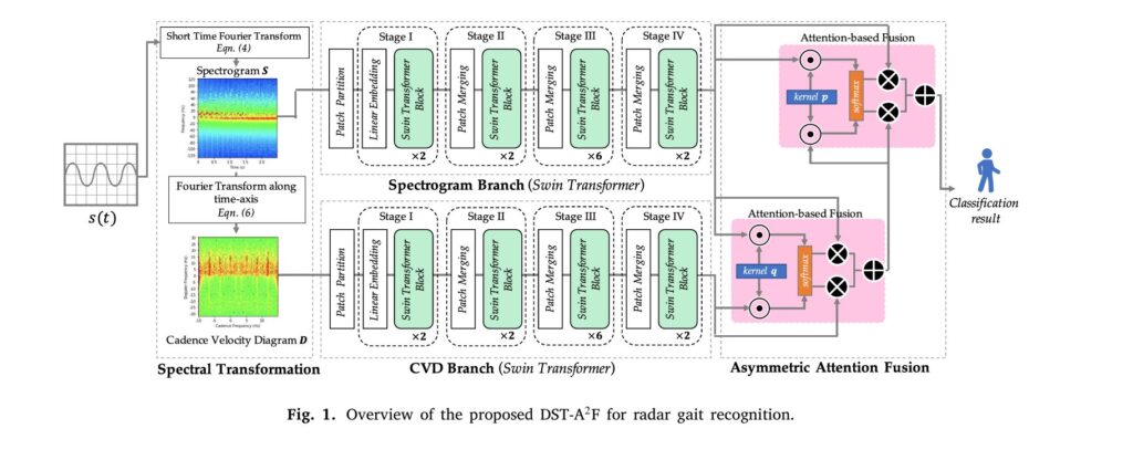
The solution lies in an unexpected direction: using radar signals to create biometric signatures based on human walking patterns. Researchers have developed a groundbreaking method called the Dual-branch Swin Transformer with Asymmetric Attention Fusion (DST-A²F), which represents a fundamental shift in how machines can identify individuals without ever recording their image. This article explores the technical innovation, practical implications, and future applications of this transformative technology.
Understanding Radar-Based Gait Recognition: The Fundamentals
Why Radar Over Video Cameras?
The advantages of radar-based gait recognition extend far beyond privacy protection. Radar has recently become increasingly popular and overcome various challenges presented by vision sensors, offering multiple compelling benefits that traditional approaches simply cannot match:
- Privacy preservation: No facial features, clothing details, or identifying visual information is recorded
- Environmental robustness: Radars work well in dim light or extreme weather conditions while video cameras cannot
- Frontal-view capability: Unlike cameras, radar effectively captures gait patterns when individuals move directly toward or away from the sensor
- Clothing invariance: Walking patterns detected through radar are unaffected by what a person is wearing
- Rapid feature extraction: Instantaneous human gait features can be extracted from radar signals, while GEIs are extracted from video sequences
Micro-Doppler Signatures: The Gait Fingerprint
At the heart of radar-based identification lies the concept of micro-Doppler signatures. When a person walks toward or away from a radar antenna, different body parts (arms, legs, torso) move at varying velocities. Each micro-motion produces distinct frequency shifts in the reflected radar signal—a phenomenon called the micro-Doppler effect. Radar micro-Doppler signature (mDS) has been widely utilized for automatic target recognition, e.g., UAV detection, pose estimation, activity recognition, and gait recognition.
Signal Processing Pipeline: From Raw Data to Spectral Representations
The transformation from raw radar signals to interpretable representations involves a sophisticated mathematical pipeline. The radar signal s(t)s(t) s(t) captured from a walking person undergoes segmentation into MM M non-overlapping segments:
where each segment xi = {xi [n],n=0,1,…,N−1} is a vector of length N. These segments form a synthetic image of size M×N. The Fourier transform is computed for each segment:
\[ f_{i,k} = \sum_{n=0}^{N-1} x_i[n] \exp\left\{-j2\pi\frac{kn}{N}\right\} \]where F{⋅} denotes the Fourier transform. The magnitude spectrum forms the spectrogram:
\[ \mathbf{S} = \{|f_{i,k}|^2, \quad i = 0, 1, \ldots, M-1, \quad k = 0, 1, \ldots, N-1\} \]For the dataset described in the paper, N=128 with a Hamming window applied. Notably, no zero-padding or window overlapping is applied to preserve temporal resolution.
The Cadence Velocity Diagram (CVD) is generated by applying a Fourier transform along the time axis of the spectrogram:
\[ \mathbf{D} = \mathcal{F}_t\{\mathbf{S}\} \]where Ft{⋅} denotes the Fourier transform along the time axis. In implementation, M=115 with a rectangle window size of 128 and zero-padding applied. The CVD describes the periodic patterns of micro-Doppler components.
Table 1: Signal Processing Parameters and Specifications
\[ \begin{array}{|l|c|c|l|} \hline \textbf{Parameter} & \textbf{Spectrogram} & \textbf{CVD} & \textbf{Physical Interpretation} \\ \hline \text{Time axis segments (M)} & 115 & 115 & \text{Number of time windows during capture} \\ \hline \text{Frequency bins (N)} & 128 & 128 & \text{Doppler frequency resolution} \\ \hline \text{Window function} & \text{Hamming} & \text{Rectangle} & \text{Spectral leakage suppression} \\ \hline \text{Sampling rate (original)} & 125\,\text{kHz} & 125\,\text{kHz} & \text{Raw signal sampling frequency} \\ \hline \text{Sampling rate (decimated)} & 1.95\,\text{kHz} & 1.95\,\text{kHz} & \text{After decimation factor of 64} \\ \hline \text{Input image size} & 115\times115 & 115\times115 & \text{Processed representation dimensions} \\ \hline \text{Resized to} & 224\times224 & 224\times224 & \text{Network input requirement} \\ \hline \text{Zero-padding} & \text{No} & \text{Yes} & \text{Temporal/frequency padding} \\ \hline \text{Window overlap} & \text{No} & \text{Yes} & \text{Spectral analysis property} \\ \hline \end{array} \]The Dual-Branch Architecture: Extracting Complementary Features
Spectrogram and Cadence Velocity Diagram Representations
The DST-A²F system processes radar data into two complementary visual representations, each capturing different aspects of gait characteristics:
Spectrograms represent the time-varying frequency content of the radar signal, showing how micro-Doppler signatures evolve throughout a complete walking cycle. They reveal fine-grained details about micro-motion patterns—the subtle velocity changes of individual body segments as a person walks.
Cadence Velocity Diagrams (CVDs), conversely, emphasize the periodic and repetitive nature of human gait. Generated by applying a Fourier transform along the time axis of the spectrogram, the CVD describes the periodic patterns of micro-Doppler components and measures how frequently different Doppler frequencies appear in the spectrogram over the observation window.
The paper illustrates this complementarity through compelling visual examples. Two individuals with superficially similar spectrograms—indicating comparable micro-motion patterns—may display distinctly different cadence patterns in their CVDs. Conversely, two people with similar cadence frequencies may reveal their differences through spectrogram details. This synergy motivated the dual-branch design.
Why Swin Transformers Excel for Radar Data
Traditional convolutional neural networks treat spectrograms as natural images, applying operations designed for photographs. However, radar representations fundamentally differ from natural images. In a photograph, objects can be translated, rotated, or scaled, but in a spectrogram, the spatial coordinates carry precise physical meaning: one axis represents Doppler frequency (velocity), and the other represents time. Feature pooling operations in DCNNs may lose this critical global positional information.
The Swin Transformer addresses this architectural mismatch through its hierarchical design and local attention mechanisms:
- Patch-based processing: The spectrogram or CVD is divided into patches, each representing a specific frequency band during a specific time interval—preserving physical meaning
- Multi-scale feature extraction: Through hierarchical stages, the network learns features at different temporal and frequency resolutions
- Shifted window attention: Instead of full self-attention across the entire image, the Swin Transformer computes attention within local windows and shifts these windows cyclically, enabling cross-window interactions while maintaining computational efficiency
- Receptive field hierarchy: Swin-T can better model local and global time–frequency features through its hierarchical design that splits and merges patches at multiple scales to extract features from multiple receptive fields
Swin Transformer Architecture Specifications
Table 2: Swin Transformer Architecture Configuration
\[ \begin{array}{|c|c|c|c|c|c|} \hline \textbf{Stage} & \textbf{Input Resolution} & \textbf{Window Size} & \textbf{Swin Block Layers} & \textbf{Heads} & \textbf{Embed Dim / Output Channels} \\ \hline 1 & 56 \times 56 & 7 \times 7 & 2 & 3 & 96 \\ \hline 2 & 28 \times 28 & 7 \times 7 & 2 & 6 & 192 \\ \hline 3 & 14 \times 14 & 7 \times 7 & 6 & 12 & 384 \\ \hline 4 & 7 \times 7 & 7 \times 7 & 2 & 24 & 768 \\ \hline \end{array} \]The patch partition mechanism divides the input spectrogram/CVD of size 224×224224 \times 224 224×224 into non-overlapping patches of size 4×44 \times 4 4×4, resulting in 56×5656 \times 56 56×56 patches. The linear embedding layer projects each patch to the embedding dimension.
Window-Based Multi-Head Self-Attention
The Swin Transformer computes attention within local windows rather than globally across the entire feature map. The attention mechanism operates as:
\[ text{Attention}(\mathbf{Q}, \mathbf{K}, \mathbf{V}) = \text{softmax}\left(\frac{\mathbf{Q}\mathbf{K}^T}{\sqrt{d_k}} + B\right)\mathbf{V} \]where Q, K, V are the query, key, and value projections, dk is the embedding dimension, and B is the relative position bias specific to each window. This local attention reduces computational complexity from O(N2) to O(NM2), where N is the number of patches and M is the window size.
Shifted window partitioning enables cross-window connections by alternating between regular and shifted window arrangements across consecutive blocks:
\[ \text{Attention}_{\text{shifted}} = \text{Attention}(\text{Shifted-Patches}) \]This mechanism allows patches to attend to neighbors in adjacent windows while maintaining the computational efficiency of local attention.
Table 3: Computational Complexity Comparison
\[ \begin{array}{|l|c|c|c|} \hline \textbf{Operation} & \textbf{Standard ViT} & \textbf{Swin Transformer} & \textbf{Reduction Factor} \\ \hline \text{Attention complexity} & O(4N^{2}) & O(4NM^{2}) & M^{2} / N \\ \hline \text{FLOPs (224 x 224 input)} & \sim 16.5\,G & \sim 5.95\,G & 2.77\times \\ \hline \text{Inference time (s)} & 109.545 & 52.16 & 2.10\times \\ \hline \text{Training time (s/epoch)} & 292.33 & 140.80 & 2.07\times \\ \hline \end{array} \]The Asymmetric Attention Fusion Mechanism
Beyond Equal-Weight Feature Combination
A critical innovation in DST-A²F lies in how it combines features from the spectrogram and CVD branches. Traditional fusion approaches treat both feature sources equally, learning to weight them based solely on input data. However, this data-driven approach overlooks valuable prior knowledge about feature importance.
Empirical studies show that the spectrogram outperforms the CVD for radar target recognition, and hence larger weights should be assigned to the spectrogram features for a better performance. Rather than forcing the network to re-discover this relationship during training, the DST-A²F architecture explicitly incorporates this knowledge.
Mathematical Framework of Asymmetric Attention Fusion
The fusion mechanism builds upon Element-wise Attention Fusion (EAF), which uses Hadamard products rather than matrix multiplication. For traditional attention-based fusion, learnable weights are derived as:
\[ w_i = \sigma(\mathbf{q}^T\mathbf{a}_i) = \frac{\exp(\mathbf{q}^T\mathbf{a}_i)}{\sum_{j}\exp(\mathbf{q}^T\mathbf{a}_j)} \]where σ(⋅) is the softmax function and q is a learnable kernel. The fusion output is derived as:
\[ \mathbf{a}_{AF} = \sum_{i=1}^{B} w_i\mathbf{a}_i \]where aAF contains partial attentive information from all B sets of features, and the optimal weights are automatically determined by the input features.
Element-wise Attention Fusion (EAF)
The EAF mechanism improves upon this by replacing matrix multiplication with Hadamard product:
\[ \mathbf{w}_i = \tilde{\sigma}(\mathbf{q} \odot \mathbf{a}_i) = \frac{\exp (\mathbf{q} \odot \mathbf{a}_i)}{\sum_{j} \exp(\mathbf{q} \odot \mathbf{a}_j)} \]where ⊙ denotes element-wise (Hadamard) production and ⊘ denotes element-wise division. The softmax function σ~ is also conducted element-wise. The fused feature is derived as:
\[ \mathbf{a}_{EAF} = \sum_{i=1}^{B} \mathbf{w}_i \odot \mathbf{a}_i \]where B=2 in the dual-branch task.
Asymmetric Attention Fusion (A²F)
The balanced fusion mechanism is well-suited when features carry equal or similar importance. However, in many tasks, prior knowledge about feature importance exists. Let EAF (fS, fD) denote the Element-wise Attention Fusion for spectrogram features fS and CVD features fD. The features fa after the proposed A²F are derived as:
\[ \mathbf{f}_a = \text{EAF}(\mathbf{f}_S, \text{EAF}(\mathbf{f}_S, \mathbf{f}_D)) \]This iterative application applies EAF with the prior knowledge that spectrogram features are more important. Since spectrogram features are weighted twice in the proposed A²F, they are assigned a higher importance than CVD features, which appear once.
Table 4: Fusion Mechanism Comparison
\[ \small \begin{array}{|l|c|c|c|c|} \hline \textbf{Fusion Method} & \textbf{Formula} & \textbf{Params} & \textbf{Weighting} & \textbf{Prior} \\ \hline \text{Concatenation} & [\mathbf{a}_1,\mathbf{a}_2] & \text{None} & \text{Equal} & \text{None} \\ \hline \text{Averaging} & \frac{1}{2}(\mathbf{a}_1+\mathbf{a}_2) & \text{None} & \text{Equal} & \text{None} \\ \hline \text{Max Pooling} & \max(\mathbf{a}_1,\mathbf{a}_2) & \text{None} & \text{Data-dep.} & \text{None} \\ \hline \text{Attention Fusion} & \sum_i w_i\mathbf{a}_i & 1 \text{ vector} & \text{Per-sample} & \text{None} \\ \hline \text{EAF} & \sum_i\mathbf{w}_i\odot\mathbf{a}_i & D & \text{Per-dim} & \text{None} \\ \hline \text{A}^{2}\text{F (Proposed)} & \text{EAF}(\mathbf{f}_S,\text{EAF}(\mathbf{f}_S,\mathbf{f}_D)) & D & \text{Per-dim} & \text{Spec.\ dom.} \\ \hline \end{array} \]The key advantage of A²F is the explicit incorporation of domain knowledge through iterative fusion, which empirical studies confirm produces superior results compared to balanced fusion approaches.
The NTU-RGR Dataset: A Large-Scale Benchmark
Dataset Construction and Protocol Design
A large-scale NTU-RGR dataset is constructed, containing 45,768 radar frames of 98 subjects. This represents a substantial resource for radar gait recognition research, collected under carefully controlled experimental conditions.
The data collection employed a 24.125 GHz K-MC1 FMCW radar transceiver in a 40-meter corridor. Each participant walked away from the radar from a starting point 0.5 meters away until reaching 25 meters distance, then returned, completing one full recording. Each recording lasted approximately 30 seconds, during which individuals were encouraged to walk naturally.
The dataset uniquely features two recording sessions separated by 7 to 62 days, deliberately introducing intra-class variations from changes in clothing, physical condition, and environmental factors—simulating real-world deployment scenarios.
Table 5: NTU-RGR Dataset Specifications
\[ \begin{array}{|l|c|l|} \hline \textbf{Property} & \textbf{Value} & \textbf{Description} \\ \hline \text{Total subjects} & 98 & \text{Diverse population (age 19–56, avg. 24)} \\ \hline \text{Recording sessions} & 2 & \text{Session 1: 98 subjects; Session 2: 69 subjects} \\ \hline \text{Total recordings} & 1,670 & \text{Complete walking sequences} \\ \hline \text{Total frames} & 45,768 & \text{After extraction with stride 10} \\ \hline \text{Frame dimensions} & 115\times115 & \text{After spectral processing} \\ \hline \text{Radar frequency} & 24.125\ \text{GHz} & \text{K-MC1 FMCW transceiver} \\ \hline \text{Radar sampling rate} & 125\ \text{kHz} & \text{Original sampling frequency} \\ \hline \text{Decimation factor} & 64 & \text{Reduces effective SR to 1.95 kHz} \\ \hline \text{Recording duration} & \sim30\ \text{s} & \text{Per complete walk cycle} \\ \hline \text{Walking distance} & 0.5{-}25\ \text{m} & \text{Away and back toward radar} \\ \hline \text{Corridor length} & 40\ \text{m} & \text{Controlled indoor environment} \\ \hline \text{Frame stride} & 10 & \text{Controls temporal overlap} \\ \hline \text{Inter-session interval} & 7{-}62\ \text{days} & \text{Clothing / condition variation} \\ \hline \end{array} \]Evaluation Protocols: Closed-Set and Open-Set Recognition
Two distinct evaluation protocols address different security scenarios:
Table 6: Evaluation Protocols and Metrics
\[ \begin{array}{|l|c|c|} \hline \textbf{Aspect} & \textbf{Closed-Set Recognition} & \textbf{Open-Set Recognition} \\ \hline \text{Description} & \text{All test subjects appear in training data} & \text{Test includes unknown imposters} \\ \hline \text{Real-world application} & \text{Authorized personnel identification} & \text{Border security, threat detection} \\ \hline \text{Training set} & \text{50\% of recordings per person (random)} & \text{Remaining recordings from Session 1} \\ \hline \text{Test set (genuine)} & \text{50\% of recordings per person} & \text{All recordings from Session 2} \\ \hline \text{Imposter set} & \text{None} & \text{Session 1 recordings not in training} \\ \hline \text{Training frames} & 18,950 & 18,950 \\ \hline \text{Test frames (genuine)} & \text{Variable} & \text{Variable} \\ \hline \text{Test frames (imposter)} & \text{N/A} & 7,868 \\ \hline \text{Evaluation metric} & \text{Rank-1 accuracy} & \text{\% genuine accepted + imposters rejected} \\ \hline \text{Difficulty level} & \text{Moderate} & \text{High (confidence-based rejection)} \\ \hline \text{Practical challenge} & \text{Recognizing known individuals} & \text{Distinguishing known vs unknown} \\ \hline \text{Number of trials} & 5\ (\text{avg.}) & 2\ (\text{protocol-specific}) \\ \hline \end{array} \]Closed-set recognition is simpler—the network only needs to correctly classify among known subjects. Open-set recognition is significantly more challenging, as it requires the model to not only recognize genuine subjects but also reject unknown imposters based on relatively low confidence scores.
Experimental Results: Achieving State-of-the-Art Performance
Comprehensive Benchmark Comparisons
The DST-A²F architecture substantially outperformed established baselines and recent methods. The proposed DST-A²F achieved 95.96% accuracy on Protocol I (closed-set) and 54.46% on Protocol II (open-set). The 7.53% improvement over ADS-ViT on Protocol I and 6.89% on Protocol II demonstrates the effectiveness of combining Swin Transformer architecture with asymmetric attention fusion.
Performance Analysis by Architecture Component
Table 8: Ablation Study Results – Component Contribution Analysis
\[ \small \begin{array}{|l|c|c|c|c|c|c|} \hline \textbf{Model Config.} & \textbf{Backbone} & \textbf{Spec} & \textbf{CVD} & \textbf{Fusion} & \textbf{Protocol I (\%)} & \textbf{Protocol II (\%)} \\ \hline \text{Baseline: Spec+ViT} & \text{ViT} & \checkmark & \times & \text{N/A} & 84.64 \pm 1.66 & 46.06 \pm 2.49 \\ \hline \text{CVD+ViT} & \text{ViT} & \times & \checkmark & \text{N/A} & 80.27 \pm 2.47 & 41.31 \pm 1.06 \\ \hline \text{Spec+Swin-T} & \text{Swin-T} & \checkmark & \times & \text{N/A} & 94.25 \pm 0.62 & 49.38 \pm 0.48 \\ \hline \text{CVD+Swin-T} & \text{Swin-T} & \times & \checkmark & \text{N/A} & 87.12 \pm 0.75 & 43.42 \pm 0.18 \\ \hline \text{ADS-ViT} & \text{ViT} & \checkmark & \checkmark & \text{EAF} & 88.43 \pm 1.03 & 47.57 \pm 0.50 \\ \hline \text{Dual-branch ViT + A^{2}F} & \text{ViT} & \checkmark & \checkmark & A^{2}F & 89.26 \pm 0.89 & 48.31 \pm 0.75 \\ \hline \text{Dual-branch Swin-T + EAF} & \text{Swin-T} & \checkmark & \checkmark & \text{EAF} & 95.01 \pm 0.45 & 52.41 \pm 0.53 \\ \hline \text{Full DST-A^{2}F} & \text{Swin-T} & \checkmark & \checkmark & A^{2}F & 95.96 \pm 0.42 & 54.46 \pm 0.67 \\ \hline \end{array} \]Key observations from the ablation study:
- Swin-T superiority: Upgrading from ViT to Swin-T improves accuracy by 9.61% on spectrograms alone and 6.85% on CVDs alone
- Fusion complementarity: Combining spectrogram and CVD branches provides 4.62% improvement over spectrogram-only with ViT and 1.71% with Swin-T
- Asymmetric advantage: A²F adds 0.95% improvement over balanced EAF on Swin-T, validating the value of incorporating prior knowledge
Backbone Architecture Comparative Analysis
Table 9: Backbone Architecture Performance Comparison
\[ \begin{array}{|l|l|c|c|c|c|} \hline \text{Backbone} & \text{Input Type} & \text{Protocol I (\%)} & \text{Protocol II (\%)} & \text{Spec vs. CVD Gap} & \text{Dual-branch Gain} \\ \hline \text{AlexNet} & \text{Spec} & 72.49 \pm 1.54 & 32.55 \pm 1.15 & -10.00 & +13.24 \\ & \text{CVD} & 82.49 \pm 1.49 & 34.29 \pm 2.93 & – & – \\ & \text{Dual} & 85.73 \pm 1.16 & 37.05 \pm 2.55 & – & – \\ \hline \text{VGG} & \text{Spec} & 78.90 \pm 1.96 & 46.38 \pm 2.09 & +6.01 & +5.19 \\ & \text{CVD} & 72.89 \pm 1.40 & 36.14 \pm 0.86 & – & – \\ & \text{Dual} & 84.09 \pm 1.07 & 46.73 \pm 1.49 & – & – \\ \hline \text{ResNet} & \text{Spec} & 86.05 \pm 1.27 & 46.48 \pm 1.69 & +5.38 & +4.63 \\ & \text{CVD} & 80.67 \pm 1.11 & 39.28 \pm 0.45 & – & – \\ & \text{Dual} & 90.68 \pm 0.91 & 47.53 \pm 1.93 & – & – \\ \hline \text{EfficientNet} & \text{Spec} & 90.92 \pm 1.07 & 47.91 \pm 1.12 & +4.81 & +2.88 \\ & \text{CVD} & 86.11 \pm 0.53 & 41.24 \pm 1.63 & – & – \\ & \text{Dual} & 93.80 \pm 0.68 & 50.01 \pm 0.45 & – & – \\ \hline \text{ViT} & \text{Spec} & 84.64 \pm 1.66 & 46.06 \pm 2.49 & +4.37 & +4.62 \\ & \text{CVD} & 80.27 \pm 2.47 & 41.31 \pm 1.06 & – & – \\ & \text{Dual} & 89.26 \pm 0.89 & 48.31 \pm 0.75 & – & – \\ \hline \text{Swin-T} & \text{Spec} & 94.25 \pm 0.62 & 49.38 \pm 0.48 & +7.13 & +1.71 \\ & \text{CVD} & 87.12 \pm 0.75 & 43.42 \pm 0.18 & – & – \\ & \text{Dual} & 95.96 \pm 0.42 & 54.46 \pm 0.67 & – & – \\ \hline \end{array} \]The analysis reveals that Swin-T achieves the best balance of accuracy and computational efficiency, with the largest spectrogram-to-CVD performance gap suggesting that the hierarchical architecture particularly benefits spectrogram feature extraction.
Fusion Mechanism Detailed Comparison
Table 10: Fusion Mechanism Performance on Dual-branch Swin-T
\[ \small \begin{array}{|l|c|c|c|c|} \hline \text{Fusion Mechanism} & \text{Protocol I Accuracy } & \text{Protocol II Accuracy } & \text{Accuracy Improvement (P1)} & \text{Accuracy Improvement (P2)} \\ \hline \text{Feature max pooling} & 94.44 \pm 0.56 & 48.85 \pm 3.88 & -1.52 & -5.61 \\ \text{Feature min pooling} & 94.42 \pm 0.63 & 49.16 \pm 2.05 & -1.54 & -5.30 \\ \text{Feature concatenation} & 94.99 \pm 0.73 & 51.87 \pm 1.63 & -0.97 & -2.59 \\ \text{Feature averaging} & 94.19 \pm 0.44 & 49.67 \pm 0.83 & -1.77 & -4.79 \\ \text{Attention-based fusion} & 93.49 \pm 2.72 & 46.89 \pm 2.19 & -2.47 & -7.57 \\ \text{EAF (Element-wise Attention)} & 95.01 \pm 0.45 & 52.41 \pm 0.53 & -0.95 & -2.05 \\ \text{A²F (Asymmetric Attention)} & 95.96 \pm 0.42 & 54.46 \pm 0.67 & \text{Baseline} & \text{Baseline} \\ \hline \end{array} \]The A²F mechanism significantly outperforms all alternatives, with the largest margins over simple fusion strategies (concatenation, averaging) and meaningful improvements over the previously best method (EAF). This validates the theoretical expectation that incorporating prior knowledge about feature importance enhances fusion effectiveness.
Cross-Dataset Validation: MMRGait-1.0 Performance
To validate generalization beyond the NTU-RGR dataset, researchers evaluated DST-A²F on the public MMRGait-1.0 benchmark.
Table 11: Multi-View Recognition Performance on MMRGait-1.0 Dataset
\[ \small \begin{array}{|l|c|c|c|c|c|} \hline \text{Wearing Condition} & \text{View Angles} & \text{ResNet50 (%)} & \text{EfficientNet (%)} & \text{ADS-ViT (%)} & \text{MS-R18-LST-SA (%)} & \text{DST-A²F (%)} \\ \hline \text{NM (Normal Wearing)} & 0^\circ & 95.74 & 93.62 & 95.74 & 91.86 & 97.87 \\ & 30^\circ & 93.62 & 89.36 & 94.68 & 94.19 & 96.80 \\ & 45^\circ & 91.49 & 96.80 & 94.68 & 96.51 & 97.87 \\ & 60^\circ & 93.62 & 92.55 & 93.62 & 94.19 & 96.80 \\ & 90^\circ & 84.04 & 82.98 & 86.17 & 91.86 & 86.17 \\ & 300^\circ & 89.36 & 90.43 & 93.62 & 98.84 & 96.80 \\ & 315^\circ & 93.62 & 91.49 & 93.62 & 91.86 & 98.94 \\ & 330^\circ & 92.55 & 90.43 & 94.68 & 96.51 & 95.74 \\ \hline \text{NM Average} & – & 91.76 & 90.96 & 93.35 & 94.48 & 95.88 \\ \hline \text{BG (Carrying Bags) Average} & – & 77.53 & 81.38 & 76.33 & 81.25 & 88.03 \\ \hline \text{CT (Wearing Coats) Average} & – & 75.80 & 76.86 & 77.93 & 79.21 & 82.98 \\ \hline \end{array} \]The proposed DST-A²F significantly outperforms others, achieving an average performance gain of 1.4% on normal wearing (NM), 6.78% on carrying bags (BG), and 3.77% on wearing coats (CT) compared to the previous best method MS-R18-LST-SA. Notably, the method struggles at 90° viewing angle where side-view gait contains fewer discriminative features, suggesting a direction for future improvement through multi-modal fusion.
Key Takeaways: Why This Matters
🎯 Privacy-First Biometrics: Unlike facial recognition or gait videos, radar-based identification requires no visual data storage, addressing the privacy concerns that plague modern surveillance systems.
🎯 All-Weather Reliability: The robustness to lighting conditions, fog, rain, and other environmental factors makes radar gait recognition viable for outdoor security applications where video fails.
🎯 Technical Innovation: The combination of Swin Transformers with asymmetric attention fusion demonstrates how architectural design can encode domain knowledge and improve performance meaningfully.
🎯 Practical Validation: Achievement of 95%+ accuracy on closed-set recognition suggests deployment readiness for authorized personnel identification in controlled environments.
Conclusion: The Future of Biometric Security
The DST-A²F architecture represents a paradigm shift in biometric authentication, prioritizing privacy, robustness, and technical sophistication over traditional video-centric approaches. By leveraging radar micro-Doppler signatures through advanced deep learning architectures, researchers have demonstrated that human identification can occur without any visual data—addressing fundamental privacy concerns while maintaining competitive accuracy.
As security systems increasingly grapple with balancing identification capability against privacy rights, radar-based gait recognition offers a compelling alternative worthy of serious consideration for access control, border security, and personnel identification applications.
What aspects of radar-based security interest you most? Are you concerned about privacy implications of traditional surveillance systems? Share your thoughts in the comments below—let’s discuss how emerging technologies can reshape security for a more privacy-respecting future.
Download the full paper and read it to click this link.
Below is the comprehensive implementation of the Dual-branch Swin Transformer with Asymmetric Attention Fusion (DST-A²F) model for radar gait recognition.
# config.py
"""
Configuration management for DST-A2F model
"""
from dataclasses import dataclass
from typing import Tuple, Optional
import yaml
import os

@dataclass
class RadarSignalConfig:
    """Radar signal processing configuration"""
    sampling_rate: int = 125000  # Original sampling rate in Hz
    decimation_factor: int = 64   # Decimation for computational efficiency
    fft_size: int = 128           # FFT window size for spectrogram
    n_segments: int = 115         # Number of time segments
    window_function: str = "hamming"  # Window type for FFT

    @property
    def effective_sampling_rate(self) -> int:
        return self.sampling_rate // self.decimation_factor

@dataclass
class DataProcessingConfig:
    """Data processing configuration"""
    spectrogram_size: Tuple[int, int] = (115, 115)
    cvd_size: Tuple[int, int] = (115, 115)
    input_size: Tuple[int, int] = (224, 224)  # Resized input for network
    num_classes: int = 98  # NTU-RGR dataset
    train_split: float = 0.5
    frame_stride: int = 10  # Stride for frame extraction

@dataclass
class ModelConfig:
    """Model architecture configuration"""
    # Swin Transformer parameters
    patch_size: int = 4
    window_size: int = 7
    embed_dim: int = 96
    depths: Tuple[int, ...] = (2, 2, 6, 2)  # Layers per stage
    num_heads: Tuple[int, ...] = (3, 6, 12, 24)  # Attention heads per stage
    mlp_ratio: float = 4.0
    dropout: float = 0.1
    attention_dropout: float = 0.0
    drop_path_rate: float = 0.2

    # Fusion parameters
    fusion_type: str = "asymmetric_attention"  # "concatenation", "attention", "asymmetric_attention"
    num_branches: int = 2

@dataclass
class TrainingConfig:
    """Training configuration"""
    batch_size: int = 32
    num_epochs: int = 150
    initial_lr: float = 1e-4
    weight_decay: float = 5e-2
    optimizer: str = "sgd"
    warmup_epochs: int = 10
    device: str = "cuda"
    num_workers: int = 4
    seed: int = 42

    # Learning rate scheduler
    scheduler: str = "cosine"  # "cosine", "step", "exponential"

    # Checkpointing
    checkpoint_dir: str = "./checkpoints"
    log_dir: str = "./logs"
    save_interval: int = 10

@dataclass
class DST_A2FConfig:
    """Complete configuration for DST-A²F model"""
    radar_signal: RadarSignalConfig = None
    data_processing: DataProcessingConfig = None
    model: ModelConfig = None
    training: TrainingConfig = None

    def __post_init__(self):
        if self.radar_signal is None:
            self.radar_signal = RadarSignalConfig()
        if self.data_processing is None:
            self.data_processing = DataProcessingConfig()
        if self.model is None:
            self.model = ModelConfig()
        if self.training is None:
            self.training = TrainingConfig()

    @classmethod
    def from_yaml(cls, yaml_path: str) -> 'DST_A2FConfig':
        """Load configuration from YAML file"""
        with open(yaml_path, 'r') as f:
            config_dict = yaml.safe_load(f)

        return cls(
            radar_signal=RadarSignalConfig(**config_dict.get('radar_signal', {})),
            data_processing=DataProcessingConfig(**config_dict.get('data_processing', {})),
            model=ModelConfig(**config_dict.get('model', {})),
            training=TrainingConfig(**config_dict.get('training', {}))
        )

    def to_yaml(self, yaml_path: str) -> None:
        """Save configuration to YAML file"""
        config_dict = {
            'radar_signal': self.radar_signal.__dict__,
            'data_processing': self.data_processing.__dict__,
            'model': self.model.__dict__,
            'training': self.training.__dict__,
        }

        os.makedirs(os.path.dirname(yaml_path), exist_ok=True)
        with open(yaml_path, 'w') as f:
            yaml.dump(config_dict, f, default_flow_style=False)


# config.yaml
radar_signal:
  sampling_rate: 125000
  decimation_factor: 64
  fft_size: 128
  n_segments: 115
  window_function: "hamming"

data_processing:
  spectrogram_size: [115, 115]
  cvd_size: [115, 115]
  input_size: [224, 224]
  num_classes: 98
  train_split: 0.5
  frame_stride: 10

model:
  patch_size: 4
  window_size: 7
  embed_dim: 96
  depths: [2, 2, 6, 2]
  num_heads: [3, 6, 12, 24]
  mlp_ratio: 4.0
  dropout: 0.1
  attention_dropout: 0.0
  drop_path_rate: 0.2
  fusion_type: "asymmetric_attention"
  num_branches: 2

training:
  batch_size: 32
  num_epochs: 150
  initial_lr: 0.0001
  weight_decay: 0.05
  optimizer: "sgd"
  warmup_epochs: 10
  device: "cuda"
  num_workers: 4
  seed: 42
  scheduler: "cosine"
  checkpoint_dir: "./checkpoints"
  log_dir: "./logs"
  save_interval: 10
# signal_processing.py
"""
Radar signal processing utilities for generating spectrograms and CVDs
"""
import numpy as np
from scipy import signal
from scipy.fft import fft, fftfreq
from typing import Tuple, Optional
import torch
class RadarSignalProcessor:
"""
Process raw radar signals into spectrograms and Cadence Velocity Diagrams
"""
def __init__(
self,
sampling_rate: int = 125000,
decimation_factor: int = 64,
fft_size: int = 128,
n_segments: int = 115,
window_type: str = "hamming"
):
"""
Initialize radar signal processor
Args:
sampling_rate: Original sampling rate in Hz
decimation_factor: Decimation factor
fft_size: FFT window size
n_segments: Number of time segments
window_type: Window function type
"""
self.sampling_rate = sampling_rate
self.decimation_factor = decimation_factor
self.effective_sr = sampling_rate // decimation_factor
self.fft_size = fft_size
self.n_segments = n_segments
self.window_type = window_type
# Create window function
self.window = signal.get_window(window_type, fft_size)
def generate_spectrogram(
self,
raw_signal: np.ndarray,
overlap: bool = False
) -> np.ndarray:
"""
Generate spectrogram from raw radar signal
Mathematical formulation:
S = {|F{x_i}|^2, i = 0, 1, ..., M-1}
where F{·} denotes Fourier transform and M is number of segments
Args:
raw_signal: Raw radar signal (1D array)
overlap: Whether to use overlapping windows
Returns:
Spectrogram of shape (n_segments, fft_size)
"""
# Decimate signal
decimated_signal = raw_signal[::self.decimation_factor]
# Segment signal
segment_length = self.fft_size
segments = []
for i in range(self.n_segments):
start_idx = i * segment_length
end_idx = start_idx + segment_length
if end_idx <= len(decimated_signal):
segment = decimated_signal[start_idx:end_idx]
segments.append(segment)
else:
# Pad with zeros if necessary
segment = np.zeros(segment_length)
valid_len = len(decimated_signal) - start_idx
if valid_len > 0:
segment[:valid_len] = decimated_signal[start_idx:]
segments.append(segment)
# Stack segments
signal_matrix = np.array(segments) # Shape: (n_segments, fft_size)
# Apply window function
windowed_signal = signal_matrix * self.window[np.newaxis, :]
# Compute FFT for each segment
fft_result = np.fft.fft(windowed_signal, axis=1)
# Compute magnitude squared
spectrogram = np.abs(fft_result) ** 2
return spectrogram.astype(np.float32)
def generate_cvd(
self,
spectrogram: np.ndarray,
zero_pad: bool = True
) -> np.ndarray:
"""
Generate Cadence Velocity Diagram (CVD) from spectrogram
Mathematical formulation:
D = F_t{S}
where F_t{·} denotes Fourier transform along time axis
Args:
spectrogram: Input spectrogram
zero_pad: Whether to apply zero-padding
Returns:
CVD of shape (n_segments, fft_size)
"""
# Apply FFT along time axis (axis 0)
if zero_pad:
# Zero-pad for spectral analysis
padded_spec = np.pad(spectrogram, ((0, self.fft_size), (0, 0)), mode='constant')
cvd_result = np.fft.fft(padded_spec, axis=0)
else:
cvd_result = np.fft.fft(spectrogram, axis=0)
# Compute magnitude
cvd = np.abs(cvd_result) ** 2
# Truncate to match input dimensions
cvd = cvd[:spectrogram.shape[0], :spectrogram.shape[1]]
return cvd.astype(np.float32)
def process_radar_frame(
self,
raw_signal: np.ndarray
) -> Tuple[np.ndarray, np.ndarray]:
"""
Process raw radar signal into spectrogram and CVD
Args:
raw_signal: Raw radar signal
Returns:
Tuple of (spectrogram, cvd)
"""
spectrogram = self.generate_spectrogram(raw_signal)
cvd = self.generate_cvd(spectrogram)
return spectrogram, cvd
def normalize_image(
self,
image: np.ndarray,
method: str = "minmax"
) -> np.ndarray:
"""
Normalize image to [0, 1] range
Args:
image: Input image
method: Normalization method ("minmax" or "standardize")
Returns:
Normalized image
"""
if method == "minmax":
min_val = image.min()
max_val = image.max()
if max_val > min_val:
return (image - min_val) / (max_val - min_val)
else:
return image
elif method == "standardize":
return (image - image.mean()) / (image.std() + 1e-7)
else:
raise ValueError(f"Unknown normalization method: {method}")
def resize_image(
self,
image: np.ndarray,
target_size: Tuple[int, int],
method: str = "bilinear"
) -> np.ndarray:
"""
Resize image to target size
Args:
image: Input image
target_size: Target size (height, width)
method: Interpolation method
Returns:
Resized image
"""
from scipy import ndimage
# Handle different interpolation methods
if method == "bilinear":
order = 1
elif method == "nearest":
order = 0
elif method == "bicubic":
order = 3
else:
order = 1
# Compute scaling factors
scale_h = target_size[0] / image.shape[0]
scale_w = target_size[1] / image.shape[1]
# Resize using scipy
resized = ndimage.zoom(image, (scale_h, scale_w), order=order)
return resized.astype(np.float32)
# Example usage
if __name__ == "__main__":
# Create processor
processor = RadarSignalProcessor(
sampling_rate=125000,
decimation_factor=64,
fft_size=128,
n_segments=115,
window_type="hamming"
)
# Generate synthetic radar signal for testing
duration = 30 # seconds
t = np.linspace(0, duration, int(125000 * duration))
# Simulate micro-Doppler signatures with multiple frequency components
raw_signal = (
np.sin(2 * np.pi * 10 * t) + # 10 Hz walking frequency
0.5 * np.sin(2 * np.pi * 20 * t) + # Arm swing
0.3 * np.sin(2 * np.pi * 30 * t) + # Torso motion
0.1 * np.random.randn(len(t)) # Noise
)
# Process signal
spectrogram, cvd = processor.process_radar_frame(raw_signal)
print(f"Spectrogram shape: {spectrogram.shape}")
print(f"CVD shape: {cvd.shape}")
# Normalize and resize
spec_norm = processor.normalize_image(spectrogram)
spec_resized = processor.resize_image(spec_norm, (224, 224))
print(f"Resized spectrogram shape: {spec_resized.shape}")# fusion.py
"""
Asymmetric Attention Fusion (A²F) mechanism
"""
import torch
import torch.nn as nn
import torch.nn.functional as F
from typing import Tuple
class ElementwiseAttentionFusion(nn.Module):
"""
Element-wise Attention Fusion (EAF)
Weights features element-wise rather than using scalar weights,
allowing different feature dimensions to have different importance.
Mathematical formulation:
w_i = σ̃(q ⊙ a_i) = exp(q ⊙ a_i) ⊘ Σ_j exp(q ⊙ a_j)
a_EAF = Σ_i w_i ⊙ a_i
where ⊙ is element-wise product, ⊘ is element-wise division,
and σ̃ is element-wise softmax
"""
def __init__(self, feature_dim: int):
"""
Initialize Element-wise Attention Fusion
Args:
feature_dim: Dimension of feature vectors
"""
super().__init__()
self.feature_dim = feature_dim
self.learnable_kernel = nn.Parameter(torch.ones(1, feature_dim))
def forward(self, features: Tuple[torch.Tensor, torch.Tensor]) -> torch.Tensor:
"""
Fuse two sets of features using element-wise attention
Args:
features: Tuple of (feature1, feature2), each of shape (B, D)
where B is batch size and D is feature dimension
Returns:
Fused features of shape (B, D)
"""
f1, f2 = features
batch_size = f1.shape[0]
# Element-wise product with learnable kernel
# w_1 = σ̃(q ⊙ f1)
w1_logits = self.learnable_kernel * f1 # (B, D)
w2_logits = self.learnable_kernel * f2 # (B, D)
# Element-wise softmax normalization
all_logits = torch.stack([w1_logits, w2_logits], dim=2) # (B, D, 2)
weights = F.softmax(all_logits, dim=2) # (B, D, 2)
w1 = weights[:, :, 0] # (B, D)
w2 = weights[:, :, 1] # (B, D)
# Fuse using element-wise products
fused = w1 * f1 + w2 * f2
return fused
class AsymmetricAttentionFusion(nn.Module):
"""
Asymmetric Attention Fusion (A²F)
Iteratively applies EAF to assign higher importance to the first branch.
This incorporates prior knowledge that one feature source is more
discriminative than the other.
Mathematical formulation:
f_a = EAF(f_S, EAF(f_S, f_D))
By applying spectrogram features (f_S) twice and CVD features (f_D) once,
spectrogram features are assigned higher importance.
"""
def __init__(self, feature_dim: int):
"""
Initialize Asymmetric Attention Fusion
Args:
feature_dim: Dimension of feature vectors
"""
super().__init__()
self.eaf = ElementwiseAttentionFusion(feature_dim)
def forward(
self,
features_primary: torch.Tensor,
features_secondary: torch.Tensor
) -> torch.Tensor:
"""
Fuse features asymmetrically, emphasizing primary features
Args:
features_primary: Primary features (e.g., spectrogram), shape (B, D)
features_secondary: Secondary features (e.g., CVD), shape (B, D)
Returns:
Fused features with asymmetric emphasis, shape (B, D)
"""
# First fusion: fuse primary and secondary
fused_1 = self.eaf((features_primary, features_secondary))
# Second fusion: fuse primary with first result
# This effectively weights primary features twice
fused_2 = self.eaf((features_primary, fused_1))
return fused_2
class AdaptiveFusion(nn.Module):
"""
Adaptive fusion mechanism that learns optimal combination strategy
"""
def __init__(
self,
feature_dim: int,
fusion_type: str = "asymmetric_attention"
):
"""
Initialize adaptive fusion
Args:
feature_dim: Dimension of feature vectors
fusion_type: Type of fusion ("concatenation", "attention",
"asymmetric_attention", "weighted_sum")
"""
super().__init__()
self.feature_dim = feature_dim
self.fusion_type = fusion_type
if fusion_type == "asymmetric_attention":
self.fusion_module = AsymmetricAttentionFusion(feature_dim)
elif fusion_type == "attention":
self.fusion_module = ElementwiseAttentionFusion(feature_dim)
elif fusion_type == "weighted_sum":
self.weight1 = nn.Parameter(torch.tensor(0.5))
self.weight2 = nn.Parameter(torch.tensor(0.5))
elif fusion_type == "concatenation":
self.fusion_module = None
else:
raise ValueError(f"Unknown fusion type: {fusion_type}")
def forward(
self,
features_1: torch.Tensor,
features_2: torch.Tensor
) -> torch.Tensor:
"""
Fuse two feature sets
Args:
features_1: First set of features
features_2: Second set of features
Returns:
Fused features
"""
if self.fusion_type == "asymmetric_attention":
return self.fusion_module(features_1, features_2)
elif self.fusion_type == "attention":
return self.fusion_module((features_1, features_2))
elif self.fusion_type == "weighted_sum":
# Normalize weights
w1 = F.softmax(torch.stack([self.weight1, self.weight2]), dim=0)[0]
w2 = F.softmax(torch.stack([self.weight1, self.weight2]), dim=0)[1]
return w1 * features_1 + w2 * features_2
elif self.fusion_type == "concatenation":
return torch.cat([features_1, features_2], dim=1)
else:
raise ValueError(f"Unknown fusion type: {self.fusion_type}")
# Test fusion modules
if __name__ == "__main__":
device = torch.device("cuda" if torch.cuda.is_available() else "cpu")
# Create test tensors
batch_size = 8
feature_dim = 768
f1 = torch.randn(batch_size, feature_dim).to(device)
f2 = torch.randn(batch_size, feature_dim).to(device)
# Test EAF
eaf = ElementwiseAttentionFusion(feature_dim).to(device)
fused_eaf = eaf((f1, f2))
print(f"EAF output shape: {fused_eaf.shape}")
# Test A²F
a2f = AsymmetricAttentionFusion(feature_dim).to(device)
fused_a2f = a2f(f1, f2)
print(f"A²F output shape: {fused_a2f.shape}")
# Test Adaptive Fusion
adaptive = AdaptiveFusion(feature_dim, "asymmetric_attention").to(device)
fused_adaptive = adaptive(f1, f2)
print(f"Adaptive fusion output shape: {fused_adaptive.shape}")# swin_transformer.py
"""
Swin Transformer implementation for radar gait recognition
"""
import torch
import torch.nn as nn
from timm.models.swin_transformer import SwinTransformer
from typing import Tuple, Optional
import torch.nn.functional as F
class SwinTransformerExtractor(nn.Module):
"""
Swin Transformer feature extractor
Extracts multi-scale features from spectrograms/CVDs using hierarchical
Swin Transformer architecture with shifted window attention.
"""
def __init__(
self,
image_size: int = 224,
patch_size: int = 4,
embed_dim: int = 96,
depths: Tuple[int, ...] = (2, 2, 6, 2),
num_heads: Tuple[int, ...] = (3, 6, 12, 24),
window_size: int = 7,
mlp_ratio: float = 4.0,
drop_rate: float = 0.0,
attn_drop_rate: float = 0.0,
drop_path_rate: float = 0.1,
num_classes: int = 1000, # Will be replaced with feature extraction
return_all_tokens: bool = False
):
"""
Initialize Swin Transformer feature extractor
Args:
image_size: Input image size
patch_size: Patch size for patch embedding
embed_dim: Embedding dimension
depths: Number of transformer blocks in each stage
num_heads: Number of attention heads in each stage
window_size: Window size for local attention
mlp_ratio: MLP hidden dim ratio
drop_rate: Dropout rate
attn_drop_rate: Attention dropout rate
drop_path_rate: Drop path rate
num_classes: Number of classes (not used, kept for compatibility)
return_all_tokens: Whether to return all feature tokens
"""
super().__init__()
# Use timm's SwinTransformer as backbone
self.swin = SwinTransformer(
img_size=image_size,
patch_size=patch_size,
embed_dim=embed_dim,
depths=depths,
num_heads=num_heads,
window_size=window_size,
mlp_ratio=mlp_ratio,
drop_rate=drop_rate,
attn_drop_rate=attn_drop_rate,
drop_path_rate=drop_path_rate,
num_classes=num_classes
)
self.return_all_tokens = return_all_tokens
self.feature_dim = embed_dim * (2 ** (len(depths) - 1)) # Final feature dimension
def forward(self, x: torch.Tensor) -> torch.Tensor:
"""
Extract features using Swin Transformer
Args:
x: Input tensor of shape (B, 3, H, W) or (B, 1, H, W)
Returns:
Feature tensor of shape (B, feature_dim) or (B, num_tokens, feature_dim)
"""
# Swin transformer expects 3-channel input, so repeat if necessary
if x.shape[1] == 1:
x = x.repeat(1, 3, 1, 1)
# Forward through swin transformer
# Remove classification head and return features
x = self.swin.patch_embed(x)
x = self.swin._pos_embed(x)
x = self.swin.patch_drop(x)
x = self.swin.layers(x)
x = self.swin.norm(x)
# Global average pooling
features = x.mean(dim=1) # (B, feature_dim)
return features
class DualBranchSwinTransformer(nn.Module):
"""
Dual-branch Swin Transformer for radar gait recognition
Processes spectrogram and CVD in parallel branches, each with
independent Swin Transformer feature extraction.
"""
def __init__(
self,
image_size: int = 224,
patch_size: int = 4,
embed_dim: int = 96,
depths: Tuple[int, ...] = (2, 2, 6, 2),
num_heads: Tuple[int, ...] = (3, 6, 12, 24),
window_size: int = 7,
mlp_ratio: float = 4.0,
drop_rate: float = 0.0,
attn_drop_rate: float = 0.0,
drop_path_rate: float = 0.1,
num_classes: int = 98
):
"""
Initialize dual-branch Swin Transformer
Args:
image_size: Input image size
patch_size: Patch size
embed_dim: Embedding dimension
depths: Depths for each stage
num_heads: Number of heads for each stage
window_size: Window size for local attention
mlp_ratio: MLP ratio
drop_rate: Dropout rate
attn_drop_rate: Attention dropout rate
drop_path_rate: Drop path rate
num_classes: Number of gait classes
"""
super().__init__()
# Spectrogram branch
self.spectrogram_branch = SwinTransformerExtractor(
image_size=image_size,
patch_size=patch_size,
embed_dim=embed_dim,
depths=depths,
num_heads=num_heads,
window_size=window_size,
mlp_ratio=mlp_ratio,
drop_rate=drop_rate,
attn_drop_rate=attn_drop_rate,
drop_path_rate=drop_path_rate,
num_classes=num_classes
)
# CVD branch
self.cvd_branch = SwinTransformerExtractor(
image_size=image_size,
patch_size=patch_size,
embed_dim=embed_dim,
depths=depths,
num_heads=num_heads,
window_size=window_size,
mlp_ratio=mlp_ratio,
drop_rate=drop_rate,
attn_drop_rate=attn_drop_rate,
drop_path_rate=drop_path_rate,
num_classes=num_classes
)
self.feature_dim = self.spectrogram_branch.feature_dim
def forward(
self,
spectrogram: torch.Tensor,
cvd: torch.Tensor
) -> Tuple[torch.Tensor, torch.Tensor]:
"""
Forward pass through dual branches
Args:
spectrogram: Spectrogram input of shape (B, 1, H, W)
cvd: CVD input of shape (B, 1, H, W)
Returns:
Tuple of (spectrogram_features, cvd_features), each of shape (B, feature_dim)
"""
spec_features = self.spectrogram_branch(spectrogram)
cvd_features = self.cvd_branch(cvd)
return spec_features, cvd_features
if __name__ == "__main__":
device = torch.device("cuda" if torch.cuda.is_available() else "cpu")
# Create dual-branch model
model = DualBranchSwinTransformer(
image_size=224,
patch_size=4,
embed_dim=96,
depths=(2, 2, 6, 2),
num_heads=(3, 6, 12, 24),
window_size=7,
num_classes=98
).to(device)
# Test with dummy inputs
batch_size = 4
spec = torch.randn(batch_size, 1, 224, 224).to(device)
cvd = torch.randn(batch_size, 1, 224, 224).to(device)
spec_feat, cvd_feat = model(spec, cvd)
print(f"Spectrogram features shape: {spec_feat.shape}")
print(f"CVD features shape: {cvd_feat.shape}")
# Count parameters
total_params = sum(p.numel() for p in model.parameters())
trainable_params = sum(p.numel() for p in model.parameters() if p.requires_grad)
print(f"Total parameters: {total_params:,}")
print(f"Trainable parameters: {trainable_params:,}")# model.py
"""
Complete DST-A²F model combining dual-branch Swin Transformer
with Asymmetric Attention Fusion
"""
import torch
import torch.nn as nn
from typing import Tuple, Optional
from swin_transformer import DualBranchSwinTransformer
from fusion import AsymmetricAttentionFusion, AdaptiveFusion
class DST_A2F(nn.Module):
"""
Dual-branch Swin Transformer with Asymmetric Attention Fusion
Complete architecture for radar gait recognition:
1. Dual-branch Swin Transformer extracts features from spectrogram and CVD
2. Asymmetric Attention Fusion combines features with prior knowledge
3. Classification head for gait identity prediction
"""
def __init__(
self,
image_size: int = 224,
patch_size: int = 4,
embed_dim: int = 96,
depths: Tuple[int, ...] = (2, 2, 6, 2),
num_heads: Tuple[int, ...] = (3, 6, 12, 24),
window_size: int = 7,
mlp_ratio: float = 4.0,
drop_rate: float = 0.0,
attn_drop_rate: float = 0.0,
drop_path_rate: float = 0.1,
num_classes: int = 98,
fusion_type: str = "asymmetric_attention",
feature_fusion_dim: Optional[int] = None
):
"""
Initialize DST-A²F model
Args:
image_size: Input image size
patch_size: Patch size
embed_dim: Embedding dimension
depths: Depths per stage
num_heads: Heads per stage
window_size: Window size
mlp_ratio: MLP ratio
drop_rate: Dropout rate
attn_drop_rate: Attention dropout rate
drop_path_rate: Drop path rate
num_classes: Number of identity classes
fusion_type: Type of fusion mechanism
feature_fusion_dim: Dimension for fusion (if None, use Swin output dim)
"""
super().__init__()
# Dual-branch Swin Transformer
self.backbone = DualBranchSwinTransformer(
image_size=image_size,
patch_size=patch_size,
embed_dim=embed_dim,
depths=depths,
num_heads=num_heads,
window_size=window_size,
mlp_ratio=mlp_ratio,
drop_rate=drop_rate,
attn_drop_rate=attn_drop_rate,
drop_path_rate=drop_path_rate,
num_classes=num_classes
)
feature_dim = self.backbone.feature_dim
fusion_dim = feature_fusion_dim if feature_fusion_dim is not None else feature_dim
# Feature projection if needed
if fusion_dim != feature_dim:
self.feature_projection = nn.Linear(feature_dim, fusion_dim)
else:
self.feature_projection = None
# Asymmetric Attention Fusion
if fusion_type == "asymmetric_attention":
self.fusion = AsymmetricAttentionFusion(fusion_dim)
else:
self.fusion = AdaptiveFusion(fusion_dim, fusion_type)
# Classification head
self.classifier = nn.Sequential(
nn.Linear(fusion_dim, fusion_dim // 2),
nn.ReLU(inplace=True),
nn.Dropout(drop_rate),
nn.Linear(fusion_dim // 2, num_classes)
)
self.num_classes = num_classes
self.feature_dim = fusion_dim
def extract_features(
self,
spectrogram: torch.Tensor,
cvd: torch.Tensor
) -> Tuple[torch.Tensor, torch.Tensor, torch.Tensor]:
"""
Extract and fuse features
Args:
spectrogram: Spectrogram input (B, 1, H, W)
cvd: CVD input (B, 1, H, W)
Returns:
Tuple of (spec_features, cvd_features, fused_features)
"""
# Extract features from both branches
spec_features, cvd_features = self.backbone(spectrogram, cvd)
# Project features if needed
if self.feature_projection is not None:
spec_features = self.feature_projection(spec_features)
cvd_features = self.feature_projection(cvd_features)
# Fuse features
if isinstance(self.fusion, AsymmetricAttentionFusion):
fused_features = self.fusion(spec_features, cvd_features)
else:
fused_features = self.fusion(spec_features, cvd_features)
return spec_features, cvd_features, fused_features
def forward(
self,
spectrogram: torch.Tensor,
cvd: torch.Tensor,
return_features: bool = False
) -> torch.Tensor | Tuple[torch.Tensor, torch.Tensor]:
"""
Forward pass
Args:
spectrogram: Spectrogram input (B, 1, H, W)
cvd: CVD input (B, 1, H, W)
return_features: Whether to return intermediate features
Returns:
Logits of shape (B, num_classes) or
Tuple of (logits, features) if return_features=True
"""
# Extract and fuse features
spec_features, cvd_features, fused_features = self.extract_features(
spectrogram, cvd
)
# Classification
logits = self.classifier(fused_features)
if return_features:
return logits, {
'spectrogram_features': spec_features,
'cvd_features': cvd_features,
'fused_features': fused_features
}
else:
return logits
# Test complete model
if __name__ == "__main__":
device = torch.device("cuda" if torch.cuda.is_available() else "cpu")
# Create model
model = DST_A2F(
image_size=224,
patch_size=4,
embed_dim=96,
depths=(2, 2, 6, 2),
num_heads=(3, 6, 12, 24),
window_size=7,
num_classes=98,
fusion_type="asymmetric_attention"
).to(device)
# Test forward pass
batch_size = 4
spec = torch.randn(batch_size, 1, 224, 224).to(device)
cvd = torch.randn(batch_size, 1, 224, 224).to(device)
# Without features
logits = model(spec, cvd)
print(f"Logits shape: {logits.shape}")
# With features
logits, features = model(spec, cvd, return_features=True)
print(f"Logits shape: {logits.shape}")
print(f"Spectrogram features shape: {features['spectrogram_features'].shape}")
print(f"CVD features shape: {features['cvd_features'].shape}")
print(f"Fused features shape: {features['fused_features'].shape}")
# Count parameters
total_params = sum(p.numel() for p in model.parameters())
print(f"\nTotal parameters: {total_params:,}")Related posts, You May like to read
- 7 Shocking Truths About Knowledge Distillation: The Good, The Bad, and The Breakthrough (SAKD)
- MOSEv2: The Game-Changing Video Object Segmentation Dataset for Real-World AI Applications
- MedDINOv3: Revolutionizing Medical Image Segmentation with Adaptable Vision Foundation Models
- HiPerformer: A New Benchmark in Medical Image Segmentation with Modular Hierarchical Fusion
- How AI is Learning to Think Before it Segments: Understanding Seg-Zero’s Reasoning-Driven Image Analysis
- SegTrans: The Breakthrough Framework That Makes AI Segmentation Models Vulnerable to Transfer Attacks
- Universal Text-Driven Medical Image Segmentation: How MedCLIP-SAMv2 Revolutionizes Diagnostic AI
- Towards Trustworthy Breast Tumor Segmentation in Ultrasound Using AI Uncertainty
- DVIS++: The Game-Changing Decoupled Framework Revolutionizing Universal Video Segmentation