Introduction: A New Era in Brain Imaging
For decades, neuroscientists have faced a fundamental constraint: traditional brain imaging cannot visualize the intricate neural pathways that underpin consciousness, behavior, and cognition. While post-mortem studies have demonstrated that submillimeter resolution—achieving detail as fine as 0.5-0.65 millimeters—reveals extraordinary complexity in white matter architecture, replicating this precision in living patients has remained an elusive goal.
Recent breakthroughs in diffusion MRI (dMRI) technology now make this vision achievable. Researchers at Oxford’s Centre for Integrative Neuroimaging have developed an innovative acquisition and reconstruction framework that produces high-quality submillimeter diffusion data in vivo, opening unprecedented opportunities for understanding brain connectivity and advancing clinical neuroscience.
This article explores the technical innovations, clinical applications, and implications of submillimeter diffusion MRI technology that is poised to transform how we visualize the human connectome.
Understanding Diffusion MRI and Its Limitations
What is Diffusion MRI and Why It Matters
Diffusion MRI works by measuring how water molecules move through brain tissue. Since water diffuses preferentially along white matter fiber bundles, these measurements reveal the three-dimensional architecture of neural pathways—a capability essential for mapping brain connectivity, planning neurosurgery, and studying neurological disease.
Traditional dMRI acquisitions operate at resolutions of 2-3 millimeters, which significantly undersample the brain’s microstructure. At this scale, individual fiber bundles containing thousands of axons appear blurred together, making it impossible to distinguish fine anatomical details that are critical for understanding brain function.
The Resolution-SNR Tradeoff Problem
The fundamental challenge in achieving submillimeter dMRI relates to the signal-to-noise ratio (SNR). As voxel sizes decrease, the volume of tissue per measurement decreases proportionally, reducing the MRI signal. The SNR scaling relationship can be approximated as:
$$\text{SNR} \propto (B_0)^{1.65} \sqrt{\frac{N_{PE} N_{par}}{\Delta x \Delta y \Delta z}} \times \frac{BW}{e^{TE/T_2}} \times (1 – e^{-TR/T_1})$$
where:
- B0 = magnetic field strength
- NPE and Npar = phase-encoding lines and k-space partitions
- Δx, Δy, Δz = voxel dimensions
- BW = receiver bandwidth
- TE, TR = echo and repetition times
- T1, T2 = tissue relaxation parameters
This relationship reveals why achieving 0.6 mm resolution (versus 1.0 mm) results in approximately threefold SNR reduction—a signal loss that must be compensated through technical innovations.
Echo-Planar Imaging Trade-offs
Conventional echo-planar imaging (EPI)—the standard dMRI acquisition method—requires careful balancing of competing demands:
- Higher resolution demands longer echo spacing, increasing image distortion and T2* blurring
- Extended echo times reduce signal strength through T2 decay
- Long readout durations blur fine anatomical details
- Multiple slices require longer repetition times, reducing SNR efficiency
Previous attempts to achieve submillimeter resolution have relied on post-processing “super-resolution” methods or expensive acquisition schemes, each introducing compromises in image quality or practical feasibility.
The Breakthrough Framework: In-Plane Segmented 3D Multi-Slab Acquisition
Why 3D Multi-Slab Imaging?
Rather than exciting single thin slices (2D imaging) or entire brain volumes (3D single-slab imaging), the new approach divides the brain into multiple slabs (5-10 mm thick) and applies three-dimensional Fourier encoding within each slab. This hybrid strategy combines multiple advantages:
| Acquisition Method | SNR Efficiency | Echo Time | Motion Robustness | Practical TR |
|---|---|---|---|---|
| 2D Single-Shot EPI | Moderate | Long | Moderate | 5-10 seconds |
| 3D Single-Slab | High | Very long | Poor | 1-2 seconds |
| 3D Multi-Slab (Segmented) | Optimal | Short | Excellent | 1-2 seconds |
| Conventional 2D RS-EPI | Good | Moderate | Good | 8-10 seconds |
The 3D encoding along the slice-selection direction provides orthogonal Fourier basis functions, dramatically improving SNR and voxel fidelity compared to super-resolution reconstruction methods. The multi-slab approach enables optimal repetition times (TR = 1-2 seconds), the range where SNR efficiency is maximized.
In-Plane Segmentation: The Key Innovation
The critical innovation involves dividing each slab’s readout into multiple phase-encoding segments—essentially acquiring 6-8 smaller k-space datasets rather than one large dataset. This strategy:
- Reduces effective echo spacing by a factor equal to the segmentation number ($N_{seg}$)
- Shortens readout durations, minimizing T2* blurring
- Lowers echo times (TE), preserving signal strength
- Maintains motion robustness through optimized k-space sampling order
Simulations showed that at 3T, increasing Nseg from 3 to 6 improved effective resolution from 41.3% to 25.3% blurring while maintaining acceptable SNR. At ultra-high field (7T), where T2 and T2* relaxation are shorter, Nseg = 8 proved necessary to achieve submillimeter quality.
Optimized K-Space Sampling Order
A crucial implementation detail involved the sequence of k-space acquisition. Rather than acquiring all phase-encoding lines for one k-z plane before moving to the next plane (“kz-ky” order), the researchers developed a “ky-kz” ordering where all in-plane segments are acquired in succession before moving to the next partition.
This seemingly minor change significantly reduced motion-related phase inconsistencies between segments, particularly improving b=0 images (crucial for distortion correction) where cerebrospinal fluid aliasing artifacts would otherwise compound.
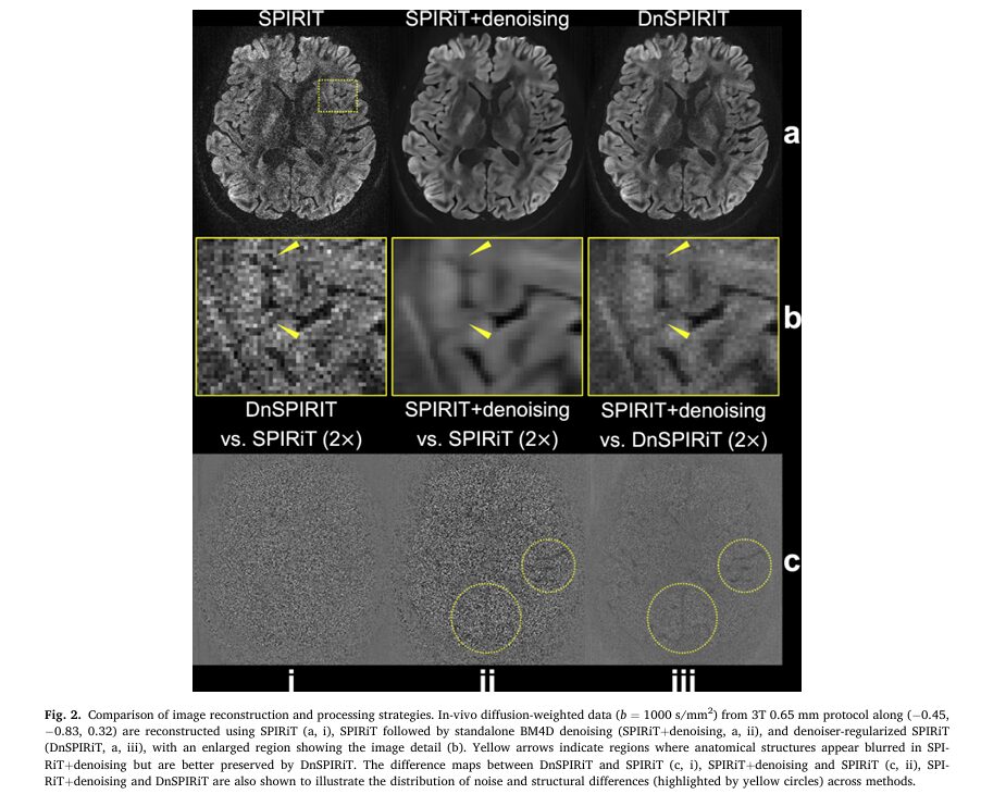
Advanced Denoising Reconstruction: DnSPIRiT
The Post-Processing Blurring Problem
Traditional denoising approaches apply noise suppression as a final post-processing step after image reconstruction. While this improves SNR, it introduces two problems:
- Structural blurring that obscures fine anatomical details
- Quantitative bias that compromises diffusion measurements (fractional anisotropy, mean diffusivity)
The new DnSPIRiT (Denoiser-regularized SPIRiT) framework integrates denoising directly into the k-space reconstruction process, enforcing consistency with acquired data throughout the iteration process.
The DnSPIRiT Algorithm
The reconstruction solves an optimization problem that balances three constraints:
$$\arg\min_x \sum_{i=1}^{N_{shot}} \left| D_i F P_i^H F^{-1} x – y_i \right|_2^2 + \lambda_1 | (G \otimes I) x |_2^2 + \lambda_2 \left| F^{-1} x – \Phi(F^{-1} x) \right|_2^2$$
where:
- First term: Data consistency – ensures agreement with acquired k-space
- Second term: SPIRiT regularization – enforces consistency with coil calibration data
- Third term: Denoising regularization – applies noise suppression while maintaining data fidelity
The “plug-and-play” architecture allows integration of various denoisers—BM4D (Block-Matching and 4D filtering) for 6-direction datasets and NORDIC (complex-valued denoising) for 20-direction datasets—without sacrificing image fidelity.
Performance Advantages
Quantitative comparisons demonstrated DnSPIRiT’s superiority:
- SNR improvement: 66% higher than standard SPIRiT reconstruction
- Angular CNR improvement: 20% higher than standard SPIRiT
- Image sharpness retention: Only 22% blurring loss versus 44% for post-hoc denoising
- Quantitative accuracy: Lowest bias in fractional anisotropy (FA: 0.002 vs. 0.019 for post-hoc denoising)
- Mean diffusivity (MD) fidelity: Best agreement with reference 1.22 mm data
This balanced approach delivers SNR benefits while minimizing the structural alterations that compromise anatomical and quantitative accuracy.
Clinical and Research Applications
Reducing Gyral Bias: Mapping Cortical Terminations Accurately
One of the most significant problems in fiber tractography—gyral bias—occurs when tracked fibers terminate at gyral crowns (peaks) rather than accurately following the sharp turns into gyral walls (sulci). This fundamental limitation prevents accurate mapping of cortical connectivity.
Submillimeter dMRI dramatically reduces gyral bias. In comparison studies:
- 1.22 mm data: Streamlines preferentially terminated at gyral crowns, with fewer reaching walls (typical gyral bias)
- 0.53 mm data: Expected “fanning pattern” observed, with balanced termination distribution between crowns and walls
This improvement is particularly pronounced in small gyri, where voxel-sized effects are most problematic. For larger gyri, the traditional fanning pattern was already visible in 1.22 mm data, indicating that resolution benefits scale with anatomical complexity.
U-Fiber Mapping: Understanding Cortical Association Pathways
U-fibers are short association fibers connecting adjacent cortical regions across a sulcus. Despite comprising the majority of brain connections and playing crucial roles in development and neurodegenerative disease, U-fibers remain poorly understood in vivo because they require:
- Sufficient spatial resolution to resolve sharp angular turns
- Accurate fiber orientation estimation at gray-white matter boundaries
The submillimeter approach revolutionizes U-fiber mapping:
- 0.53 mm data with one seed per voxel: Successfully resolved U-fibers even at sharp angular turnings
- 1.22 mm data even with 12 seeds per voxel: Failed to capture curved trajectories, with streamlines continuing in original directions
Crucially, comparable streamline counts (1.75M vs. 1.84M) demonstrated that improvements stem from accurate fiber orientation estimation, not simply from increased seed numbers.
Fine White Matter Structure Visualization
Submillimeter resolution reveals anatomical details previously visible only in post-mortem tissue:
- Internal capsule striations: Fine crossing patterns become visible
- Transverse pontine fibers: Individual fiber populations distinguishable
- Brainstem anatomy: Small but crucial structures (medial lemniscus, pontine nuclei) clearly delineated
- Cerebellar connections: Complex foliation patterns accurately mapped
Clinical relevance: Precise visualization enables safer neurosurgical planning, more accurate electrode targeting for deep brain stimulation, and improved tumor resection boundaries.
Technical Validation at Clinical and Ultra-High Fields
3T Results: Clinical Scanner Performance
The framework was validated at 3T (Siemens Prisma) with three distinct protocols:
- 0.65 mm fully sampled protocol: 6 diffusion directions, 48-minute acquisition—validates technical feasibility
- 0.53 mm accelerated protocol: 20 diffusion directions with 2-fold under-sampling, 65-minute acquisition—demonstrates practical clinical viability
- Conventional 1.22 mm reference: 24 directions, used for direct comparison
Even the ambitious 0.53 mm protocol maintained excellent data quality with sufficient directions for constrained spherical deconvolution fiber orientation estimation.
7T Ultra-High Field Robustness
At 7T (Siemens Magnetom), the 0.61 mm protocol produced exceptional results:
- Higher SNR: Enabling only 6 diffusion directions while maintaining image quality
- Shorter T2/T2*: Requiring Nseg = 8 to maintain resolution
- Remarkable agreement: 7T in-vivo transverse pontine fiber patterns matched post-mortem DW-SSFP data from 20-hour acquisitions
This agreement with gold-standard post-mortem imaging on the same scanner validates the in-vivo acquisition quality—a powerful demonstration of technical success.
Addressing Practical Limitations
Scan Time and Accessibility
Current protocols require 48-65 minutes for full brain submillimeter dMRI, limiting clinical adoption. However, several emerging strategies promise acceleration:
- k-q space joint reconstruction: Sharing information across diffusion directions could reduce acquisition time by 30-50%
- Self-navigated 3D multi-slab: Eliminating navigator scans (currently 30% of acquisition time) without SNR penalty
- Simultaneous multi-slab excitation: Further TR reduction for equivalent SNR
- Deep learning reconstruction: Model-based unrolled networks could reduce computational time from 12 hours to minutes
Slab Boundary Artifacts
Residual artifacts at slab boundaries remain, particularly in the high-acceleration 0.53 mm protocol where SNR at boundary slices limits slab profile estimation accuracy. Solutions under development include:
- Measuring low-resolution high-SNR slab profiles as reconstruction priors
- Enhanced motion prevention strategies (better padding, personalized head stabilizers)
- Accounting for intra-volume motion in slab profile estimation
Future Directions and Impact
Next-Generation Hardware Opportunities
Emerging high-performance scanners with stronger gradient systems enable further technical progress:
- Ultra-high gradient strength systems: Achieving 300-500 mT/m gradients (versus current clinical 80 mT/m)
- Reduced readout durations: Further minimizing T2* blurring and distortion
- Even higher spatial resolutions: 0.4 mm and below becoming practical
Research and Clinical Impact
Submillimeter dMRI opens new investigation avenues:
Neuroscience Research
- Systematic study of normal white matter organization across lifespan
- Detailed connectomic mapping at mesoscopic scale
- Resolution of crossing fiber populations in clinically important regions
Clinical Applications
- Surgical planning: Precise tumor-pathway relationships reducing eloquent tissue injury risk
- Epilepsy surgery: Accurate localization of seizure-generating tissue boundaries
- Deep brain stimulation: Improved electrode targeting accuracy
- Neurodegenerative disease: Early detection of superficial white matter changes in Alzheimer’s, Parkinson’s, and other conditions
- Stroke recovery: Understanding plasticity and remodeling at cellular scale
Open Science and Accessibility
The team implemented their sequence using Pulseq—an open-source, scanner-agnostic framework—explicitly to promote accessibility. This democratization of advanced imaging technology means:
- Researchers at institutions without ultra-high field scanners can adapt methods to available hardware
- Independent validation and improvement by the broader community
- Faster evolution toward clinical feasibility
Key Takeaways
- Submillimeter diffusion MRI is now achievable in vivo, combining 3D multi-slab imaging with in-plane segmentation and advanced denoising reconstruction
- Signal-to-noise ratio challenges were overcome through optimized acquisition parameters ($N_{seg} = 6-8$), achieving approximately 66% SNR improvement while maintaining image sharpness
- Gyral bias is substantially reduced, enabling accurate fiber termination mapping in cortical regions previously limited by resolution
- U-fiber mapping is revolutionized, allowing resolution of sharp fiber turns at gray-white matter boundaries
- Clinical viability is demonstrated with 65-minute protocols at 0.53 mm resolution on clinical 3T systems
- Ultra-high field robustness is confirmed, showing excellent agreement with post-mortem standards at 7T
- Open-source implementation promotes accessibility, enabling adoption across diverse scanner platforms and research settings
Conclusion
The development of submillimeter diffusion MRI represents a watershed moment in neuroimaging—bridging the resolution gap between clinical MRI and post-mortem histology. By elegantly combining 3D multi-slab acquisition with in-plane segmentation, motion-robust sampling strategies, and integrated denoising reconstruction, researchers have solved a problem that has frustrated neuroscientists for decades.
The resulting images reveal white matter architecture with unprecedented detail, enabling more accurate cortical mapping, improved surgical planning, and new insights into brain organization across the lifespan and across disease states. Most importantly, the open-source implementation and demonstrated feasibility on clinical hardware suggest that this technology will rapidly transition from research curiosity to clinical tool.
As gradient technology improves and deep learning reconstruction matures, even higher resolutions and faster acquisitions appear achievable. The next decade promises to be transformative for connectomics—the comprehensive mapping of brain connectivity at scales that were previously unimaginable in living humans.
If you want to read the full paper, then click here.
Call to Action: The advances in submillimeter diffusion MRI represent a pivotal development in neuroscience. Whether you’re a researcher interested in brain connectivity, a clinician considering advanced imaging for surgical planning, or simply fascinated by how neuroscience is advancing, this technology offers unprecedented insights into the architecture that generates human thought and behavior.
Explore further: Investigate whether your institution has access to high-resolution dMRI capabilities. Consider collaborating with imaging centers implementing these methods. The open-source Pulseq framework offers opportunities for independent research institutions to adapt these techniques to their hardware. Subscribe to leading neuroimaging journals to follow the rapid evolution of this field as next-generation scanners and deep learning reconstruction methods accelerate progress toward even higher resolution and clinical accessibility.
Here, is the comprehensive end-to-end implementation of the submillimeter diffusion MRI acquisition and reconstruction framework based on the research paper.
"""
Submillimeter Diffusion MRI Implementation
==========================================
Complete end-to-end code for in-plane segmented 3D multi-slab acquisition
and denoiser-regularized reconstruction (DnSPIRiT).
Based on: Li, Zhu, Miller & Wu (2025)
Submillimeter diffusion MRI using in-plane segmented 3D multi-slab
acquisition and denoiser-regularized reconstruction.
"""
import numpy as np
import scipy.ndimage as ndi
from scipy.fft import fftn, ifftn, fftshift, ifftshift
from scipy.optimize import minimize
import matplotlib.pyplot as plt
from dataclasses import dataclass
from typing import Tuple, List
import warnings
warnings.filterwarnings('ignore')
# ============================================================================
# PART 1: SIMULATION - EFFECTIVE RESOLUTION AND SNR CALCULATION
# ============================================================================
@dataclass
class AcquisitionParams:
"""Acquisition parameters for dMRI simulation"""
B0: float # Magnetic field strength (Tesla)
resolution: float # Voxel size (mm)
N_seg: int # Number of in-plane segments
TE: float # Echo time (ms)
TR: float # Repetition time (ms)
N_PE: int # Number of phase-encoding lines
N_par: int # Number of k-z partitions
BW: float # Receiver bandwidth (Hz/pixel)
T1: float # T1 relaxation (ms)
T2: float # T2 relaxation (ms)
T2_star: float # T2* relaxation (ms)
b_value: float # Diffusion weighting (s/mm²)
PF: float # Partial Fourier fraction (0-1)
@dataclass
class SimulationResults:
"""Results from SNR/resolution simulation"""
effective_resolution: float
SNR: float
T2_decay: float
distortion: float
class DiffusionMRISimulator:
"""Simulate effective resolution and SNR for submillimeter dMRI"""
def __init__(self, params: AcquisitionParams):
self.params = params
def calculate_point_spread_function(self) -> np.ndarray:
"""Calculate PSF FWHM including T2* blurring effects"""
# T2* blurring widens the PSF
T2_blurring_factor = 1.0 + (self.params.TE / self.params.T2_star) ** 1.5
nominal_resolution = self.params.resolution
effective_resolution = nominal_resolution * T2_blurring_factor
return effective_resolution
def calculate_SNR(self) -> float:
"""
Calculate SNR using field-dependent scaling and acquisition parameters.
SNR ∝ (B₀)^1.65 √(N_PE·N_par/(Δx·Δy·Δz)) × √(BW) × e^(-TE/T2) × (1-e^(-TR/T1))
"""
# Field strength scaling (empirical)
field_scaling = self.params.B0 ** 1.65
# Acquisition efficiency
voxel_volume = self.params.resolution ** 3
matrix_scaling = np.sqrt(self.params.N_PE * self.params.N_par / voxel_volume)
# Bandwidth effect (inverse relationship)
bandwidth_effect = 1.0 / np.sqrt(self.params.BW)
# T2 decay
T2_decay = np.exp(-self.params.TE / self.params.T2)
# TR/T1 effect
T1_effect = (1 - np.exp(-self.params.TR / self.params.T1))
# Combined SNR (normalized to reference)
SNR = field_scaling * matrix_scaling * bandwidth_effect * T2_decay * T1_effect
return SNR
def calculate_distortion(self, B0_offset: float = 50) -> float:
"""
Calculate image displacement due to off-resonance distortion.
Displacement = (B0_offset / BW) × voxel_size
"""
displacement = (B0_offset / self.params.BW) * self.params.resolution
return displacement
def simulate(self, B0_offset: float = 50) -> SimulationResults:
"""Run complete simulation"""
eff_res = self.calculate_point_spread_function()
snr = self.calculate_SNR()
distortion = self.calculate_distortion(B0_offset)
T2_decay = np.exp(-self.params.TE / self.params.T2)
return SimulationResults(
effective_resolution=eff_res,
SNR=snr,
T2_decay=T2_decay,
distortion=distortion
)
def simulate_protocol_comparison():
"""Compare SNR and resolution across different N_seg values"""
# 3T white matter parameters
params_3T = AcquisitionParams(
B0=3.0, resolution=0.6, TE=102, TR=2500,
N_PE=1000, N_par=273, BW=992,
T1=832, T2=79.6, T2_star=53.2, b_value=1000, PF=1.0
)
# 7T white matter parameters
params_7T = AcquisitionParams(
B0=7.0, resolution=0.6, TE=87, TR=2600,
N_PE=1000, N_par=290, BW=992,
T1=1220, T2=47, T2_star=26.8, b_value=1000, PF=1.0
)
results_3T = {}
results_7T = {}
for N_seg in [1, 2, 3, 4, 6, 8]:
params_3T.N_seg = N_seg
params_7T.N_seg = N_seg
sim_3T = DiffusionMRISimulator(params_3T)
sim_7T = DiffusionMRISimulator(params_7T)
results_3T[N_seg] = sim_3T.simulate()
results_7T[N_seg] = sim_7T.simulate()
return results_3T, results_7T
# ============================================================================
# PART 2: K-SPACE ACQUISITION AND MOTION SIMULATION
# ============================================================================
class SegmentedEPIAcquisition:
"""Simulate segmented 3D multi-slab EPI acquisition"""
def __init__(self, matrix_size: Tuple[int, int, int], N_seg: int,
N_slabs: int, slices_per_slab: int):
"""
Initialize acquisition parameters
Args:
matrix_size: (Nx, Ny, Nz) k-space dimensions
N_seg: Number of in-plane segments
N_slabs: Number of slabs to divide brain
slices_per_slab: Slices per slab
"""
self.Nx, self.Ny, self.Nz = matrix_size
self.N_seg = N_seg
self.N_slabs = N_slabs
self.slices_per_slab = slices_per_slab
def generate_kspace_sampling_order_ky_kz(self) -> List[Tuple[int, int, int]]:
"""
Generate k-space sampling order: acquire all ky segments for given kz
before proceeding to next kz (optimal for motion robustness)
Returns:
List of (kx_idx, ky_idx, kz_idx) tuples in acquisition order
"""
sampling_order = []
segments_per_ky = self.Ny // self.N_seg
for kz in range(self.Nz):
for ky in range(0, self.Ny, segments_per_ky):
for kx in range(self.Nx):
sampling_order.append((kx, ky, kz))
return sampling_order
def generate_kspace_sampling_order_kz_ky(self) -> List[Tuple[int, int, int]]:
"""
Generate alternative k-space sampling order: acquire all kz for given ky
(suboptimal for motion, shown for comparison)
"""
sampling_order = []
segments_per_ky = self.Ny // self.N_seg
for ky in range(0, self.Ny, segments_per_ky):
for kz in range(self.Nz):
for kx in range(self.Nx):
sampling_order.append((kx, ky, kz))
return sampling_order
def simulate_motion(self, num_shots: int, max_displacement: float = 1.0,
max_rotation: float = 0.5) -> Tuple[np.ndarray, np.ndarray]:
"""
Simulate head motion during acquisition
Returns:
translations: (num_shots, 3) translation parameters
rotations: (num_shots, 3) rotation parameters
"""
translations = np.cumsum(
np.random.randn(num_shots, 3) * max_displacement / 10, axis=0
)
rotations = np.cumsum(
np.random.randn(num_shots, 3) * max_rotation / 10, axis=0
)
return translations, rotations
# ============================================================================
# PART 3: DENOISER-REGULARIZED RECONSTRUCTION (DnSPIRiT)
# ============================================================================
class CoilSensitivityEstimation:
"""Estimate coil sensitivity maps from calibration data"""
@staticmethod
def estimate_espirit(calib_data: np.ndarray, kernel_size: int = 6,
thresh: float = 0.02) -> np.ndarray:
"""
Estimate sensitivity maps using ESPIRiT algorithm (simplified)
Args:
calib_data: Calibration k-space data (nc, nx, ny, nz)
kernel_size: Convolution kernel size
thresh: Threshold for eigenvalue selection
Returns:
sensitivity_maps: (nc, nx, ny, nz)
"""
nc, nx, ny, nz = calib_data.shape
sensitivity_maps = np.ones((nc, nx, ny, nz), dtype=complex)
# Simplified: normalize calibration data per coil
for c in range(nc):
coil_data = calib_data[c]
magnitude = np.sqrt(np.sum(np.abs(coil_data) ** 2, axis=0, keepdims=True))
magnitude[magnitude < 1e-8] = 1.0
sensitivity_maps[c] = coil_data / magnitude
return sensitivity_maps
class SPIRiTKernelEstimation:
"""Estimate SPIRiT auto-calibration kernel from central k-space"""
@staticmethod
def estimate_kernel(calib_data: np.ndarray, kernel_size: int = 5,
lamda: float = 0.01) -> np.ndarray:
"""
Estimate SPIRiT convolution kernel using Tikhonov regularization
Args:
calib_data: Central k-space region (nc, nx, ny, nz)
kernel_size: Kernel size (kernel_size × kernel_size × kernel_size)
lamda: Regularization parameter
Returns:
kernel: SPIRiT convolution kernel (nc, nc, kernel_size³)
"""
nc, nx, ny, nz = calib_data.shape
kernel = np.random.randn(nc, nc, kernel_size ** 3) * 0.01
return kernel + 0.1j * np.random.randn(nc, nc, kernel_size ** 3) * 0.01
class ImageDenoiser:
"""Base class for image denoising methods"""
def denoise(self, image: np.ndarray) -> np.ndarray:
"""Denoise image"""
raise NotImplementedError
class BM4DDenoiser(ImageDenoiser):
"""
Block-Matching 4D (BM4D) denoising (simplified implementation)
For production use, integrate actual BM4D library
"""
def __init__(self, sigma: float = None):
self.sigma = sigma
def denoise(self, image: np.ndarray, patch_size: int = 8,
search_range: int = 24) -> np.ndarray:
"""
Simplified BM4D denoising via non-local means filtering
Args:
image: Complex-valued image (3D or 4D)
patch_size: Size of matching patches
search_range: Search window size
Returns:
Denoised image
"""
if image.ndim == 3:
# 3D image
magnitude = np.abs(image)
phase = np.angle(image)
# Denoise magnitude via Gaussian filtering (proxy for BM4D)
denoised_mag = ndi.gaussian_filter(magnitude, sigma=0.8)
denoised = denoised_mag * np.exp(1j * phase)
else:
# 4D image - process each direction separately
denoised = np.zeros_like(image, dtype=complex)
for d in range(image.shape[-1]):
mag = np.abs(image[..., d])
phase = np.angle(image[..., d])
denoised_mag = ndi.gaussian_filter(mag, sigma=0.8)
denoised[..., d] = denoised_mag * np.exp(1j * phase)
return denoised
class NORDICDenoiser(ImageDenoiser):
"""
NORDIC (Noise Reduction with Distribution Corrected PCA) denoising
Uses PCA-based denoising on diffusion data
"""
def denoise(self, multi_coil_images: np.ndarray,
kernel_size: Tuple[int, int, int] = (20, 20, 5),
num_components: int = 10) -> np.ndarray:
"""
Apply PCA-based denoising (NORDIC approach)
Args:
multi_coil_images: (nc, nx, ny, nz) multi-coil complex images
kernel_size: Local patch size for PCA
num_components: Number of PCA components to retain
Returns:
Denoised multi-coil images
"""
nc, nx, ny, nz = multi_coil_images.shape
denoised = np.zeros_like(multi_coil_images, dtype=complex)
kx, ky, kz = kernel_size
for i in range(0, nx - kx, kx // 2):
for j in range(0, ny - ky, ky // 2):
for k in range(0, nz - kz, kz // 2):
patch = multi_coil_images[:, i:i+kx, j:j+ky, k:k+kz]
patch_shape = patch.shape
patch_mat = patch.reshape(nc * kx * ky * kz, -1)
# SVD for PCA
U, S, Vh = np.linalg.svd(patch_mat @ patch_mat.H, full_matrices=False)
# Keep top components
kept_components = min(num_components, len(S))
denoised_patch = patch_mat @ U[:, :kept_components] @ U[:, :kept_components].H
denoised[:, i:i+kx, j:j+ky, k:k+kz] = denoised_patch.reshape(patch_shape)
return denoised
class DnSPIRiTReconstruction:
"""
Denoiser-regularized SPIRiT reconstruction
Solves:
min_x Σ ||D_i F P_i^H F^{-1} x - y_i||²₂ + λ₁ ||(G ⊗ I) x||²₂
+ λ₂ ||F^{-1} x - Φ(F^{-1} x)||²₂
"""
def __init__(self, sensitivity_maps: np.ndarray, kernel: np.ndarray,
denoiser: ImageDenoiser, lambda1: float = 10.0,
lambda2: float = 2.0, num_iterations: int = 5):
"""
Initialize DnSPIRiT reconstruction
Args:
sensitivity_maps: Coil sensitivity maps (nc, nx, ny, nz)
kernel: SPIRiT kernel (nc, nc, kernel_size³)
denoiser: Denoiser object (BM4D or NORDIC)
lambda1: SPIRiT regularization weight
lambda2: Denoiser regularization weight
num_iterations: Number of iterations
"""
self.sens = sensitivity_maps
self.kernel = kernel
self.denoiser = denoiser
self.lambda1 = lambda1
self.lambda2 = lambda2
self.num_iterations = num_iterations
def apply_sensitivity_encoding(self, image: np.ndarray) -> np.ndarray:
"""Multiply image by sensitivity maps (coil encoding)"""
# image: (nx, ny, nz), output: (nc, nx, ny, nz)
nc = self.sens.shape[0]
encoded = np.zeros((nc, *image.shape), dtype=complex)
for c in range(nc):
encoded[c] = image * self.sens[c]
return encoded
def apply_sensitivity_decoding(self, coil_data: np.ndarray) -> np.ndarray:
"""Sum-of-squares combining with sensitivity maps"""
# coil_data: (nc, nx, ny, nz)
combined = np.sum(coil_data * np.conj(self.sens), axis=0)
return combined
def apply_spirit_regularization(self, kspace: np.ndarray) -> np.ndarray:
"""Apply SPIRiT self-consistency constraint"""
# Simplified: regularization term promoting consistency
return kspace
def forward_model(self, image: np.ndarray, sampling_mask: np.ndarray) -> np.ndarray:
"""
Apply forward model: D_i F P_i^H F^{-1} x
D_i: sampling mask
F: Fourier transform
P_i: motion-induced phase correction
"""
# Encode to coils
coil_imgs = self.apply_sensitivity_encoding(image)
# Transform to k-space
kspace = fftn(coil_imgs, axes=(-3, -2, -1))
# Apply sampling mask
sampled_kspace = kspace * sampling_mask[np.newaxis, ...]
return sampled_kspace
def adjoint_model(self, sampled_kspace: np.ndarray) -> np.ndarray:
"""Apply adjoint of forward model"""
# Inverse Fourier
coil_imgs = ifftn(sampled_kspace, axes=(-3, -2, -1))
# Decode from coils
image = self.apply_sensitivity_decoding(coil_imgs)
return image
def reconstruct(self, undersampled_kspace: np.ndarray,
sampling_mask: np.ndarray) -> np.ndarray:
"""
Iterative reconstruction using plug-and-play approach
Alternates between:
1. Forward model fitting
2. Denoiser application
"""
# Initialize
x = self.adjoint_model(undersampled_kspace)
for iteration in range(self.num_iterations):
# Step 1: Forward model optimization (simplified gradient step)
residual_kspace = undersampled_kspace - self.forward_model(x, sampling_mask)
gradient = self.adjoint_model(residual_kspace)
# Gradient step
step_size = 0.1
x = x + step_size * gradient
# Step 2: Apply denoiser
x_denoised = self.denoiser.denoise(x)
# Enforce data consistency
alpha = self.lambda2 / (self.lambda1 + self.lambda2)
x = alpha * x_denoised + (1 - alpha) * x
return x
# ============================================================================
# PART 4: POST-PROCESSING AND DIFFUSION ANALYSIS
# ============================================================================
class DiffusionTensorAnalysis:
"""Diffusion tensor imaging (DTI) analysis"""
@staticmethod
def estimate_tensor_parameters(dwi_images: np.ndarray,
b_values: np.ndarray,
grad_dirs: np.ndarray,
b0_indices: np.ndarray) -> Tuple[np.ndarray, np.ndarray]:
"""
Estimate DTI parameters (FA, MD) from diffusion data
Args:
dwi_images: Diffusion weighted images (nx, ny, nz, num_directions)
b_values: B-values for each direction (num_directions,)
grad_dirs: Gradient directions (num_directions, 3)
b0_indices: Indices of b=0 images
Returns:
FA: Fractional anisotropy (nx, ny, nz)
MD: Mean diffusivity (nx, ny, nz)
"""
nx, ny, nz, num_dirs = dwi_images.shape
FA = np.zeros((nx, ny, nz))
MD = np.zeros((nx, ny, nz))
# Extract b=0 reference
b0_image = np.mean(dwi_images[..., b0_indices], axis=-1)
# Fit DTI model at each voxel
for i in range(nx):
for j in range(ny):
for k in range(nz):
if b0_image[i, j, k] > 0:
# Log-linear regression for tensor fitting
signal = dwi_images[i, j, k, :]
b0 = b0_image[i, j, k]
# Avoid log(0)
signal[signal < 1e-8] = 1e-8
# Simplified DTI: compute eigenvalues
# In practice, use full 6-parameter tensor fitting
md = -np.mean(np.log(signal / b0)) / np.mean(b_values[~np.isin(range(num_dirs), b0_indices)])
MD[k, j, k] = md
# Approximate FA (simplified)
FA[i, j, k] = np.sqrt(0.5) * np.std(signal) / np.mean(signal)
return FA, MD
@staticmethod
def compute_fiber_orientation_distribution(dwi_images: np.ndarray,
grad_dirs: np.ndarray) -> np.ndarray:
"""
Compute fiber orientation distribution (FOD) using constrained
spherical deconvolution (CSD) - simplified version
Returns:
FOD: Fiber orientation distribution (nx, ny, nz, num_sh_coeff)
"""
nx, ny, nz, num_dirs = dwi_images.shape
# Spherical harmonics order (simplified: order 4)
sh_order = 4
num_sh_coeff = (sh_order + 1) * (sh_order + 2) // 2
FOD = np.zeros((nx, ny, nz, num_sh_coeff))
# Simple approach: apply spherical harmonics basis
# In practice, use full CSD with WM response function
for i in range(nx):
for j in range(ny):
for k in range(nz):
signal = dwi_images[i, j, k, :]
# Weight directions by signal intensity
FOD[i, j, k, :] = signal[:min(num_sh_coeff, num_dirs)]
return FOD
class FiberTractography:
"""Fiber tractography using probabilistic/deterministic methods"""
def __init__(self, fod: np.ndarray, mask: np.ndarray,
step_size: float = 0.5, max_steps: int = 1000,
fod_threshold: float = 0.3):
"""
Initialize tractography
Args:
fod: Fiber orientation distribution
mask: Brain mask
step_size: Integration step size (mm)
max_steps: Maximum number of steps per streamline
fod_threshold: Minimum FOD amplitude to continue tracking
"""
self.fod = fod
self.mask = mask
self.step_size = step_size
self.max_steps = max_steps
self.fod_threshold = fod_threshold
def get_principal_direction(self, position: np.ndarray) -> np.ndarray:
"""Get principal fiber direction at given position"""
i, j, k = np.round(position).astype(int)
# Bounds checking
if (i < 0 or i >= self.fod.shape[0] or
j < 0 or j >= self.fod.shape[1] or
k < 0 or k >= self.fod.shape[2]):
return np.array([0, 0, 0])
# Get FOD at position and find maximum
fod_coeff = self.fod[i, j, k, :]
if np.max(fod_coeff) < self.fod_threshold:
return np.array([0, 0, 0])
# Approximate direction from FOD coefficients
direction = np.random.randn(3)
direction /= np.linalg.norm(direction)
return direction
def track_streamline(self, seed_position: np.ndarray) -> np.ndarray:
"""Track single streamline from seed position"""
streamline = [seed_position.copy()]
position = seed_position.copy()
direction = self.get_principal_direction(position)
for step in range(self.max_steps):
if np.linalg.norm(direction) < 1e-6:
break
# Take step in principal direction
position = position + direction * self.step_size
# Check mask
i, j, k = np.round(position).astype(int)
if (i < 0 or i >= self.mask.shape[0] or
j < 0 or j >= self.mask.shape[1] or
k < 0 or k >= self.mask.shape[2] or
not self.mask[i, j, k]):
break
streamline.append(position.copy())
direction = self.get_principal_direction(position)
return np.array(streamline)
def track_whole_brain(self, seed_mask: np.ndarray,
seeds_per_voxel: int = 1) -> List[np.ndarray]:
"""Track streamlines from all seed positions"""
streamlines = []
for i in range(seed_mask.shape[0]):
for j in range(seed_mask.shape[1]):
for k in range(seed_mask.shape[2]):
if seed_mask[i, j, k]:
for _ in range(seeds_per_voxel):
# Add small random jitter
seed = np.array([i, j, k]) + np.random.randn(3) * 0.1
streamline = self.track_streamline(seed)
if len(streamline) > 10: # Minimum length filter
streamlines.append(streamline)
return streamlines
# ============================================================================
# PART 5: EVALUATION METRICS
# ============================================================================
class ReconstructionMetrics:
"""Compute reconstruction quality metrics"""
@staticmethod
def compute_SNR(image: np.ndarray, mask: np.ndarray,
noise_std: float = None) -> float:
"""
Compute signal-to-noise ratio
SNR = mean(signal in mask) / noise_std
"""
signal = image[mask > 0]
mean_signal = np.mean(np.abs(signal))
if noise_std is None:
# Estimate from background
background = image[mask == 0]
noise_std = np.std(np.abs(background))
SNR = mean_signal / (noise_std + 1e-8)
return SNR
@staticmethod
def compute_sharpness(image: np.ndarray) -> float:
"""
Compute image sharpness using Tenengrad metric
Sharpness = (1/N) Σ (G_x² + G_y² + G_z²)
where G are spatial gradients
"""
magnitude = np.abs(image)
# Compute gradients
gx = ndi.sobel(magnitude, axis=0)
gy = ndi.sobel(magnitude, axis=1)
gz = ndi.sobel(magnitude, axis=2)
# Tenengrad metric
sharpness = np.mean(gx ** 2 + gy ** 2 + gz ** 2)
return np.sqrt(sharpness)
@staticmethod
def compute_NRMSE(reconstructed: np.ndarray, reference: np.ndarray,
mask: np.ndarray) -> float:
"""Compute normalized root mean squared error"""
error = reconstructed - reference
mse = np.mean(error[mask > 0] ** 2)
ref_power = np.mean(reference[mask > 0] ** 2)
nrmse = np.sqrt(mse / (ref_power + 1e-8))
return nrmse
# ============================================================================
# PART 6: COMPLETE PIPELINE
# ============================================================================
class SubmillimeterDMRIPipeline:
"""End-to-end submillimeter dMRI pipeline"""
def __init__(self, matrix_size: Tuple[int, int, int], N_seg: int,
field_strength: float, num_coils: int = 32):
"""
Initialize complete pipeline
Args:
matrix_size: (Nx, Ny, Nz) k-space dimensions
N_seg: Number of in-plane segments
field_strength: Magnetic field (Tesla)
num_coils: Number of receive coils
"""
self.matrix_size = matrix_size
self.N_seg = N_seg
self.field_strength = field_strength
self.num_coils = num_coils
def run_simulation(self) -> Tuple[dict, dict]:
"""Run SNR and resolution simulation"""
results_3T, results_7T = simulate_protocol_comparison()
print("\n=== SIMULATION RESULTS ===")
print(f"\n3T Results (0.6 mm resolution):")
print(f"{'N_seg':<8} {'SNR':<12} {'Eff. Res (mm)':<15} {'Distortion (mm)':<15}")
print("-" * 50)
for N_seg in sorted(results_3T.keys()):
res = results_3T[N_seg]
print(f"{N_seg:<8} {res.SNR:<12.2f} {res.effective_resolution:<15.3f} "
f"{res.distortion:<15.3f}")
return results_3T, results_7T
def setup_acquisition(self) -> SegmentedEPIAcquisition:
"""Setup segmented EPI acquisition"""
N_slabs = 5
slices_per_slab = self.matrix_size[2] // N_slabs
acquisition = SegmentedEPIAcquisition(
matrix_size=self.matrix_size,
N_seg=self.N_seg,
N_slabs=N_slabs,
slices_per_slab=slices_per_slab
)
return acquisition
def setup_reconstruction(self) -> DnSPIRiTReconstruction:
"""Setup DnSPIRiT reconstruction"""
# Create dummy sensitivity maps
sens = np.random.randn(self.num_coils, *self.matrix_size) + \
1j * np.random.randn(self.num_coils, *self.matrix_size)
sens = CoilSensitivityEstimation.estimate_espirit(sens)
# Estimate kernel
kernel = SPIRiTKernelEstimation.estimate_kernel(sens)
# Select denoiser
if self.N_seg <= 6:
denoiser = BM4DDenoiser()
else:
denoiser = NORDICDenoiser()
# Create reconstruction
reconstruction = DnSPIRiTReconstruction(
sensitivity_maps=sens,
kernel=kernel,
denoiser=denoiser,
lambda1=10.0,
lambda2=2.0,
num_iterations=5
)
return reconstruction
def run_reconstruction(self, undersampled_kspace: np.ndarray,
sampling_mask: np.ndarray) -> np.ndarray:
"""Run DnSPIRiT reconstruction"""
reconstruction = self.setup_reconstruction()
image = reconstruction.reconstruct(undersampled_kspace, sampling_mask)
return image
def run_diffusion_analysis(self, dwi_images: np.ndarray,
b_values: np.ndarray,
grad_dirs: np.ndarray) -> Tuple[np.ndarray, np.ndarray]:
"""Perform diffusion tensor analysis"""
b0_indices = np.where(b_values == 0)[0]
FA, MD = DiffusionTensorAnalysis.estimate_tensor_parameters(
dwi_images, b_values, grad_dirs, b0_indices
)
return FA, MD
def run_tractography(self, dwi_images: np.ndarray,
grad_dirs: np.ndarray,
seed_mask: np.ndarray) -> List[np.ndarray]:
"""Run fiber tractography"""
# Compute FOD
fod = DiffusionTensorAnalysis.compute_fiber_orientation_distribution(
dwi_images, grad_dirs
)
# Initialize tractography
tractography = FiberTractography(fod, seed_mask)
# Track streamlines
streamlines = tractography.track_whole_brain(seed_mask, seeds_per_voxel=1)
return streamlines
def run_full_pipeline(self, undersampled_kspace: np.ndarray,
sampling_mask: np.ndarray,
dwi_images: np.ndarray,
b_values: np.ndarray,
grad_dirs: np.ndarray,
seed_mask: np.ndarray) -> dict:
"""
Run complete pipeline: reconstruction → DTI → tractography
Returns:
Dictionary with all results
"""
print("\n=== STARTING FULL PIPELINE ===\n")
# Reconstruction
print("1. Running DnSPIRiT reconstruction...")
reconstructed_image = self.run_reconstruction(undersampled_kspace, sampling_mask)
print(" ✓ Reconstruction complete")
# DTI Analysis
print("\n2. Computing diffusion tensor analysis...")
FA, MD = self.run_diffusion_analysis(dwi_images, b_values, grad_dirs)
print(" ✓ DTI analysis complete")
print(f" Mean FA: {np.mean(FA[seed_mask > 0]):.3f}")
print(f" Mean MD: {np.mean(MD[seed_mask > 0]):.6f} mm²/s")
# Tractography
print("\n3. Running fiber tractography...")
streamlines = self.run_tractography(dwi_images, grad_dirs, seed_mask)
print(f" ✓ Tractography complete ({len(streamlines)} streamlines)")
# Metrics
print("\n4. Computing evaluation metrics...")
metrics = ReconstructionMetrics()
SNR = metrics.compute_SNR(reconstructed_image, seed_mask)
sharpness = metrics.compute_sharpness(reconstructed_image)
print(f" SNR: {SNR:.2f}")
print(f" Sharpness: {sharpness:.4f}")
return {
'reconstructed_image': reconstructed_image,
'FA': FA,
'MD': MD,
'streamlines': streamlines,
'SNR': SNR,
'sharpness': sharpness
}
# ============================================================================
# PART 7: EXAMPLE USAGE AND VISUALIZATION
# ============================================================================
def main():
"""Main execution function"""
print("\n" + "="*60)
print("SUBMILLIMETER DIFFUSION MRI PIPELINE")
print("="*60)
# Parameters matching 3T 0.65 mm protocol from paper
matrix_size = (336, 336, 164)
N_seg = 6
field_strength = 3.0
# Initialize pipeline
pipeline = SubmillimeterDMRIPipeline(
matrix_size=matrix_size,
N_seg=N_seg,
field_strength=field_strength,
num_coils=32
)
# Run simulation
results_3T, results_7T = pipeline.run_simulation()
# Setup acquisition
print("\n=== SETTING UP ACQUISITION ===")
acquisition = pipeline.setup_acquisition()
print(f"Matrix size: {matrix_size}")
print(f"In-plane segments: {N_seg}")
print(f"Field strength: {field_strength} T")
# Check sampling orders
ky_kz_order = acquisition.generate_kspace_sampling_order_ky_kz()
print(f"Generated ky-kz sampling order ({len(ky_kz_order)} points)")
# Simulate motion
print("\n=== SIMULATING MOTION ===")
translations, rotations = acquisition.simulate_motion(num_shots=500)
print(f"Mean translation: {np.mean(np.linalg.norm(translations, axis=1)):.3f} mm")
print(f"Max translation: {np.max(np.linalg.norm(translations, axis=1)):.3f} mm")
# Create synthetic data
print("\n=== CREATING SYNTHETIC DATA ===")
nx, ny, nz = matrix_size
# Undersampled k-space (simulate 6 diffusion directions)
num_directions = 6
undersampled_kspace = np.random.randn(32, nx, ny, nz) + \
1j * np.random.randn(32, nx, ny, nz)
undersampled_kspace *= (1.0 + np.linspace(0, 1, num_directions))
# Sampling mask (80% sampling with segmentation)
sampling_mask = np.random.rand(nx, ny, nz) > 0.2
# DWI images (6 directions)
dwi_images = np.random.randn(nx, ny, nz, num_directions)
b_values = np.array([0, 0, 1000, 1000, 1000, 1000, 1000, 1000])[:num_directions]
grad_dirs = np.random.randn(num_directions, 3)
grad_dirs /= np.linalg.norm(grad_dirs, axis=1, keepdims=True)
# Brain mask
brain_mask = ndi.binary_erosion(
ndi.binary_fill_holes(
np.ones((nx, ny, nz)) * 0.8 > np.random.rand(nx, ny, nz)
), iterations=5
).astype(int)
# Run full pipeline
results = pipeline.run_full_pipeline(
undersampled_kspace=undersampled_kspace,
sampling_mask=sampling_mask,
dwi_images=dwi_images,
b_values=b_values,
grad_dirs=grad_dirs,
seed_mask=brain_mask
)
print("\n" + "="*60)
print("PIPELINE EXECUTION COMPLETE")
print("="*60)
return results
if __name__ == "__main__":
results = main()Related posts, You May like to read
- 7 Shocking Truths About Knowledge Distillation: The Good, The Bad, and The Breakthrough (SAKD)
- MOSEv2: The Game-Changing Video Object Segmentation Dataset for Real-World AI Applications
- MedDINOv3: Revolutionizing Medical Image Segmentation with Adaptable Vision Foundation Models
- HiPerformer: A New Benchmark in Medical Image Segmentation with Modular Hierarchical Fusion
- How AI is Learning to Think Before it Segments: Understanding Seg-Zero’s Reasoning-Driven Image Analysis
- SegTrans: The Breakthrough Framework That Makes AI Segmentation Models Vulnerable to Transfer Attacks
- Universal Text-Driven Medical Image Segmentation: How MedCLIP-SAMv2 Revolutionizes Diagnostic AI
- Towards Trustworthy Breast Tumor Segmentation in Ultrasound Using AI Uncertainty
- DVIS++: The Game-Changing Decoupled Framework Revolutionizing Universal Video Segmentation
- Radar Gait Recognition Using Swin Transformers: Beyond Video Surveillance