TRINet: How Advanced AI Is Revolutionizing Personalized Breast Cancer Risk Prediction

Introduction

Breast cancer remains one of the most prevalent health concerns affecting women worldwide, yet early detection through personalized screening can dramatically improve outcomes. Traditional breast cancer screening protocols rely on generic, one-size-fits-all approaches that often result in either unnecessary anxiety through false positives or dangerous delays in detection. A groundbreaking new deep learning system called TRINet (Time-decay Radiomics Integrated Network) is transforming how artificial intelligence predicts individual breast cancer risk by incorporating temporal changes in breast tissue, radiomic biomarkers, and machine learning sophistication previously unseen in cancer screening applications.

Unlike conventional models that analyze individual mammograms in isolation, TRINet examines the progression of breast tissue over multiple screening intervals, enabling radiologists to recommend truly personalized screening schedules that protect high-risk patients while sparing low-risk individuals from unnecessary radiation exposure. Recent evaluation demonstrates that TRINet achieves AUC (Area Under the Receiver Operating Characteristic Curve) scores of 0.851 for one-year predictions and maintains performance above 0.789 across five-year forecasting intervals—representing a meaningful advancement in clinical decision-making accuracy.

Understanding the Limitations of Current Breast Cancer Screening

The One-Size-Fits-All Problem

Current screening mammography guidelines, while well-intentioned, struggle with a fundamental contradiction. Healthcare organizations like the American Cancer Society and American College of Physicians recommend regular screening on fixed schedules, yet these standardized protocols fail to account for individual risk variation. This creates two equally problematic scenarios:

Over-screening: Low-risk women undergo unnecessary mammograms, accumulating radiation exposure, experiencing false-positive anxiety, and facing potential overtreatment
Under-screening: High-risk women miss critical early detection windows when intervention is most effective, leading to cancers discovered at advanced stages

Traditional statistical risk models, including the Tyrer-Cuzick model, Gail model, and Breast Cancer Surveillance Consortium assessments, incorporate demographic factors and family history but achieve only moderate discriminatory power with AUC results below 70 percent. These models cannot capture the dynamic nature of breast tissue changes that occur throughout a woman’s life due to hormone therapy, lifestyle modifications, aging, and other physiological factors.

Why Image-Based Deep Learning Represents Progress

Recent research has demonstrated that deep learning models analyzing mammographic images directly significantly outperform traditional statistical approaches, achieving AUC results above 80 percent. However, even these advanced systems suffer from a critical oversight: they analyze single static images without considering temporal progression.

As cancer develops over years—not days—the sequential patterns visible across multiple screening mammograms contain invaluable diagnostic information. The breakthrough insight driving TRINet’s development is that newer mammographic images carry more relevance for current risk assessment than older screening exams, much like how radiologists themselves emphasize recent images when making clinical decisions.

The TRINet Architecture: Four Game-Changing Innovations

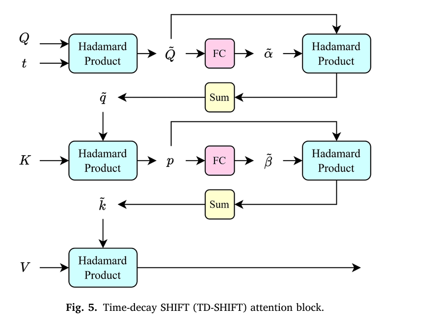
1. Time-Decay Attention for Sequential Analysis

TRINet introduces a sophisticated temporal attention mechanism that fundamentally differs from conventional image analysis approaches. Rather than weighting all prior mammograms equally, the model applies an exponential decay function to older screening exams, progressively reducing their influence on risk predictions.

The mathematical foundation employs negative exponential decay applied to query and key attention matrices:

$$t = \frac{1}{e^{A + B\Delta t_{i,n}}}$$

Where:

A and B are calibrated parameters (optimal values: A = 2.0, B = 0.1)
Δt_{i,n} represents the time interval in months between earlier image i and the most recent image n
T is a threshold (optimally set to 60 months, equivalent to five years)

This formulation ensures that a mammogram from two years ago receives substantially less attention weight than one from six months ago. Remarkably, this time-decay mechanism improved one-year AUC scores from 0.825 to 0.851—a clinically meaningful improvement that could alter screening recommendations for thousands of patients.

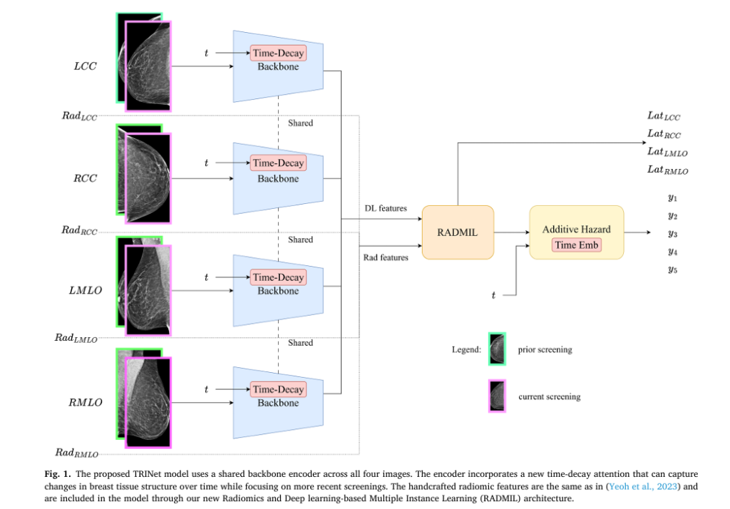
2. RADMIL: Intelligent Integration of Radiomic and Deep Learning Features

Traditional machine learning approaches simply concatenate handcrafted radiomic features (texture patterns, density measurements, shape characteristics) with deep learning-extracted features in fully-connected layers. TRINet introduces RADMIL (Radiomics and Deep learning-based Multiple Instance Learning), which treats radiomic features as equally sophisticated as neural network features.

The RADMIL framework employs attention-based aggregation:

$$z = \sum_{k=1}^{n} a_k h_k$$

$$a_k = \frac{\exp(FC_2(\tanh(FC_1(h_k))))}{\sum_{j=1}^{n}\exp(FC_2(\tanh(FC_1(h_j))))}$$

Where each feature receives an importance weight (a_k) that the network learns during training. Configuration E—which separately processes radiomic features through fully-connected layers while processing deep learning features through AMIL, then intelligently combines both outputs—demonstrated the highest performance, with 1-year AUC of 0.852.

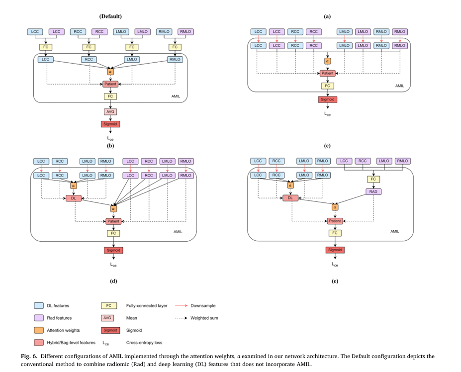
This approach offers two critical advantages:

Improved Accuracy: Features work synergistically rather than in isolation, capturing complementary information
Enhanced Interpretability: Clinicians can understand which views (mediolateral oblique vs. craniocaudal) and feature types most influence risk predictions

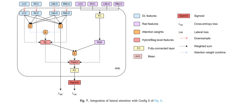
3. Lateral Attention for Bilateral Asymmetry Detection

Cancer typically develops in only one breast, yet many risk models overlook this critical asymmetry characteristic. TRINet incorporates supervised lateral attention that trains the model to identify which breast demonstrates concerning changes:

$$l_k = \sigma(FC_{l2}(\tanh(FC_{l1}(h_k))))$$

$$a = \frac{a_k l_k}{\sum_{i} a_i l_i}$$

Where σ represents a sigmoid function that produces attention scores ranging from 0 to 1 for each breast. The model learns to allocate near-zero attention to normal breast tissue while emphasizing affected breast regions. This bilateral asymmetry measurement aligns with decades of clinical observation and improves model performance across 4 of 5 prediction intervals.

4. ReST_CL: Continual Learning Without Catastrophic Forgetting

A revolutionary advancement in TRINet is its ability to learn from new populations without forgetting knowledge gained from previous training cohorts. The ReST_CL (Reinforced Self-Training with Continual Learning) approach uses an innovative label assignment strategy based on bilateral asymmetry differences:

$$\Delta A(x) = |A(x_L) – A(x_R)| = |(A(x_{LCC}) + A(x_{LMLO})) – (A(x_{RCC}) + A(x_{RMLO}))|$$

High-confidence samples (those falling in the 99th percentile for cases or 1st percentile for controls) receive hard labels during secondary dataset training, while uncertain samples receive soft pseudo-labels. This approach enabled TRINet to improve performance on Swedish CSAW dataset samples by 0.8549 AUC (one-year) without degrading performance on the original American EMBED dataset—a technical achievement previously unseen in breast cancer risk prediction.

Time-Interval Embeddings: Enabling Personalized Screening Schedules

Perhaps the most clinically transformative innovation is TRINet’s integration of time-interval embeddings into an additive hazard layer, enabling predictions across six-month intervals from immediate risk through five-year horizons.

The enhanced additive hazard formulation:

$$P(\text{cancer} = T|x) = B(AMIL(m,r)) + \sum_{i=1}^{T} H_i(AMIL(m,r) + e(t))$$

Where:

B(x) represents baseline risk
H_i(x) represents marginal hazard for each time interval
e(t) provides temporal context through learned embeddings
AMIL(m,r) combines deep learning features (m) and radiomic features (r)

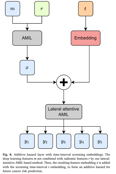
Results demonstrate that time-interval embeddings improved 1-year AUC from 0.857 to 0.865 and 2-year AUC from 0.814 to 0.817. This enables radiologists to recommend truly personalized screening: high-risk women with significant short-term cancer probability can return in six months, while low-risk women can safely extend screening to three years, reducing cumulative radiation exposure and healthcare costs.

Clinical Performance: Validation Across Diverse Populations

TRINet was evaluated on two large, diverse datasets:

EMBED Dataset (American cohort): 8,528 participants including 116,000 mammographic images representing diverse racial and ethnic backgrounds (African American, Caucasian, Asian, Native Hawaiian populations). This dataset includes longitudinal follow-up data spanning years, capturing real-world screening intervals.

CSAW Dataset (Swedish cohort): 8,723 participants from Stockholm region spanning 2008-2016. As a secondary population enabling continual learning evaluation, this cohort demonstrates generalizability across geographic and healthcare system variations.

Prediction Interval	TRINet AUC	95% Confidence Interval
1-year	0.8549	0.815–0.904
2-year	0.8139	0.769–0.863
3-year	0.8014	0.759–0.851
4-year	0.7971	0.754–0.841
5-year	0.7934	0.752–0.838

When compared with reimplemented state-of-the-art methods (Mirai, LoMaR), TRINet demonstrated significantly higher 2- to 5-year AUC results than LoMaR (p < 0.007) and significantly higher 1- and 2-year results than Mirai (p < 0.0007 and p = 0.040, respectively).

Implementation Insights and Technical Requirements

TRINet employs a ResNet18 convolutional neural network backbone—a choice validated by ablation studies showing superior performance compared to AlexNet or VGG16. The system processes four mammographic images (craniocaudal and mediolateral oblique views for both breasts) through shared encoder layers incorporating time-decay attention mechanisms.

Key technical specifications:

Input Resolution: 256 × 256 pixels (balancing computational feasibility with information retention)
Training Strategy: Two-phase learning rate approach (5e-4 for rapid adaptation, 5e-5 for fine-tuning)
Optimization: Adam optimizer with continual learning phases using vanilla SGD
Computational Resources: Dual RTX 2080 Ti GPUs with 12GB memory each

The two-phase learning rate strategy proved essential, as models trained with single lower learning rates achieved only 0.813 one-year AUC compared to 0.821 with the dual-rate approach, demonstrating the importance of gradual adaptation to temporal attention mechanisms.

Clinical Translation and Practical Impact

The implications for clinical practice are profound. Rather than recommending all women return annually or biennially, radiologists can now counsel patients based on individualized risk trajectories:

Very high short-term risk (1-year AUC > 0.90): Return in 6 months
Elevated short-term risk (1-year AUC 0.75–0.90): Return in 1 year
Moderate risk (1-year AUC 0.60–0.75): Return in 2 years
Low risk (1-year AUC < 0.60): Return in 3 years

This personalization reduces unnecessary radiation exposure while improving detection rates through intensified monitoring of truly vulnerable populations.

Future Directions and Ongoing Research

While TRINet demonstrates impressive performance on American and Swedish cohorts, evaluation on additional diverse populations—particularly Asian, African, and Latin American communities—would strengthen clinical applicability and address known disparities in cancer screening outcomes. Prospective clinical trials comparing TRINet-guided screening intervals against conventional protocols would provide definitive evidence of clinical utility and patient outcomes.

Additionally, integration of TRINet with emerging imaging modalities (tomosynthesis, supplemental ultrasound) and molecular biomarkers (circulating tumor DNA, imaging proteomics) represents a logical next frontier for enhanced risk stratification.

Conclusion and Call to Action

TRINet represents a meaningful advance in artificial intelligence application to cancer screening, addressing fundamental limitations of existing approaches through temporal attention, intelligent feature integration, bilateral asymmetry detection, and continual learning capabilities. By enabling truly personalized screening schedules, this technology has potential to improve cancer detection rates while reducing unnecessary screening burden—ultimately saving lives while decreasing healthcare costs.

For radiologists, healthcare administrators, and technology leaders committed to advancing breast cancer detection: Explore how time-decay radiomics integrated networks might enhance your screening programs. Engage with your institutional research teams to evaluate implementation feasibility. Consider participating in prospective studies validating personalized screening protocols. The evidence supporting individualized, AI-guided screening is compelling—the time to transition from population-based protocols to precision oncology is now.

Request a consultation with your institution’s radiology and informatics leadership to discuss TRINet integration pathways for your patient population.

The full paper is available here. (https://www.sciencedirect.com/science/article/pii/S1361841525003755)

Below is a comprehensive implementation of the proposed TRINET architecture.

"""
TRINet: Time-decay Radiomics Integrated Network for Breast Cancer Risk Prediction
Full end-to-end implementation
"""

import torch
import torch.nn as nn
import torch.optim as optim
from torch.utils.data import Dataset, DataLoader
import numpy as np
from typing import Tuple, List, Optional
import torch.nn.functional as F


# ============================================================================
# 1. TIME-DECAY ATTENTION MECHANISMS
# ============================================================================

class TimeDecayNonLocal(nn.Module):
    """Time-decay Non-Local attention block (TD-NL)"""
    
    def __init__(self, channels, reduction=8, A=2.0, B=0.1, T=60):
        super(TimeDecayNonLocal, self).__init__()
        self.channels = channels
        self.reduction = reduction
        self.A = A
        self.B = B
        self.T = T
        
        # Query, Key, Value projections (1x1 convolutions)
        self.query = nn.Conv2d(channels, channels // reduction, 1)
        self.key = nn.Conv2d(channels, channels // reduction, 1)
        self.value = nn.Conv2d(channels, channels // reduction, 1)
        self.out = nn.Conv2d(channels // reduction, channels, 1)
        
    def compute_time_decay(self, time_intervals, device):
        """Compute time-decay weights using exponential decay
        
        Args:
            time_intervals: Tensor of shape (batch, time_points) with time gaps in months
            device: Device to place tensor on
            
        Returns:
            decay_weights: Tensor of shape (batch, time_points)
        """
        # Clip time intervals to threshold T
        time_clipped = torch.clamp(time_intervals, max=self.T)
        # Normalize by T to [0, 1]
        time_normalized = time_clipped / self.T
        # Apply exponential decay: 1 / exp(A + B*t)
        decay_weights = 1.0 / torch.exp(self.A + self.B * time_normalized)
        return decay_weights
    
    def forward(self, x, time_intervals):
        """
        Args:
            x: Input tensor (batch, channels, height, width, time)
            time_intervals: Time differences from current scan (batch, time)
        """
        b, c, h, w, t = x.shape
        device = x.device
        
        # Process through time dimension
        Q = self.query(x.view(b * t, c, h, w)).view(b, t, -1, h, w)
        K = self.key(x.view(b * t, c, h, w)).view(b, t, -1, h, w)
        V = self.value(x.view(b * t, c, h, w)).view(b, t, -1, h, w)
        
        # Compute time decay weights
        decay = self.compute_time_decay(time_intervals, device)  # (b, t)
        
        # Apply Hadamard product with decay weights
        decay_expanded = decay.view(b, t, 1, 1, 1)
        Q_decayed = Q * decay_expanded  # (b, t, c, h, w)
        K_decayed = K * decay_expanded
        
        # Reshape for attention computation
        Q_flat = Q_decayed.view(b * t, -1, h * w).permute(0, 2, 1)  # (bt, hw, c)
        K_flat = K_decayed.view(b * t, -1, h * w)  # (bt, c, hw)
        V_flat = V.view(b * t, -1, h * w)  # (bt, c, hw)
        
        # Compute attention
        attn = torch.bmm(Q_flat, K_flat)  # (bt, hw, hw)
        attn = torch.softmax(attn / np.sqrt(self.channels), dim=-1)
        
        # Apply attention to values
        out = torch.bmm(V_flat, attn.permute(0, 2, 1))  # (bt, c, hw)
        out = out.view(b, t, -1, h, w)
        
        # Aggregate across time and project
        out = out.mean(dim=1)  # (b, c, h, w)
        out = out.view(b * 1, -1, h, w)
        out = self.out(out)
        
        return out.view(b, self.channels, h, w)


class TimeDecaySHIFT(nn.Module):
    """Time-decay SHIFT attention block (TD-SHIFT) - Linear complexity version"""
    
    def __init__(self, channels, A=2.0, B=0.1, T=60):
        super(TimeDecaySHIFT, self).__init__()
        self.channels = channels
        self.A = A
        self.B = B
        self.T = T
        
        self.fc_q = nn.Linear(channels, channels)
        self.fc_k = nn.Linear(channels, channels)
        self.fc_v = nn.Linear(channels, channels)
        
    def compute_time_decay(self, time_intervals, device):
        """Compute exponential time decay"""
        time_clipped = torch.clamp(time_intervals, max=self.T)
        time_normalized = time_clipped / self.T
        decay_weights = 1.0 / torch.exp(self.A + self.B * time_normalized)
        return decay_weights
    
    def forward(self, x, time_intervals):
        """
        Args:
            x: (batch, channels, height, width, time) or (batch, channels, time)
            time_intervals: (batch, time)
        """
        b, c, *spatial_time = x.shape
        device = x.device
        
        # Flatten spatial dimensions
        if len(spatial_time) == 3:  # height, width, time
            h, w, t = spatial_time
            x_flat = x.permute(0, 4, 1, 2, 3).reshape(b * t, c, h * w)
        else:  # just time
            t = spatial_time[0]
            x_flat = x.permute(0, 2, 1)  # (b, t, c)
        
        # Compute Q, K, V
        Q = self.fc_q(x_flat)  # (b*t or b, spatial, c)
        K = self.fc_k(x_flat)
        V = self.fc_v(x_flat)
        
        # Compute time decay
        decay = self.compute_time_decay(time_intervals, device)  # (b, t)
        
        # Apply decay only to query
        if len(spatial_time) == 3:
            decay_expanded = decay.view(b, t, 1).repeat(1, 1, h * w).reshape(b * t, 1)
        else:
            decay_expanded = decay.view(b * t, 1)
        
        Q_decayed = Q * decay_expanded
        
        # Global query and key
        q_global = Q_decayed.mean(dim=-2 if len(spatial_time) == 3 else 1, keepdim=True)
        k_global = K.mean(dim=-2 if len(spatial_time) == 3 else 1, keepdim=True)
        
        # Compute attention with reduced complexity
        attn_q = torch.softmax(self.fc_q(q_global), dim=-1)
        attn_k = torch.softmax(self.fc_k(k_global), dim=-1)
        
        # Weight value
        out = V * attn_k
        
        return out


# ============================================================================
# 2. RADIOMIC FEATURES EXTRACTION
# ============================================================================

class RadiomicFeatureExtractor(nn.Module):
    """Extract handcrafted radiomic features from mammograms"""
    
    def __init__(self, num_features=64):
        super(RadiomicFeatureExtractor, self).__init__()
        self.num_features = num_features
    
    def extract_texture_features(self, image):
        """Extract first-order and second-order texture features"""
        # First-order statistics
        mean = image.mean()
        std = image.std()
        skewness = ((image - mean) ** 3).mean() / (std ** 3)
        kurtosis = ((image - mean) ** 4).mean() / (std ** 4)
        
        # Histogram features
        hist, _ = np.histogram(image.detach().cpu().numpy().flatten(), bins=256)
        hist = hist / hist.sum()
        entropy = -np.sum(hist * np.log(hist + 1e-10))
        
        return torch.tensor([mean, std, skewness, kurtosis, entropy], 
                           dtype=image.dtype, device=image.device)
    
    def extract_density_features(self, image):
        """Extract breast density-related features"""
        # Percentage density
        threshold = image.mean()
        dense_region = (image > threshold).float()
        density_percentage = dense_region.mean()
        
        # Spatial distribution
        density_std = dense_region.std()
        
        return torch.tensor([density_percentage, density_std],
                           dtype=image.dtype, device=image.device)
    
    def extract_morphological_features(self, image):
        """Extract shape and morphological features"""
        # Edge detection using Sobel
        dx = image[:, :, 1:] - image[:, :, :-1]
        dy = image[:, 1:, :] - image[:, :-1, :]
        edges = torch.sqrt(dx[:, :, :-1] ** 2 + dy[:, :-1, :] ** 2)
        
        edge_intensity = edges.mean()
        edge_count = (edges > edges.mean()).sum().float()
        
        return torch.tensor([edge_intensity, edge_count],
                           dtype=image.dtype, device=image.device)
    
    def forward(self, image):
        """
        Args:
            image: Tensor of shape (batch, height, width)
        Returns:
            features: Tensor of shape (batch, num_features)
        """
        batch_size = image.shape[0]
        all_features = []
        
        for i in range(batch_size):
            img = image[i]
            texture = self.extract_texture_features(img)
            density = self.extract_density_features(img)
            morpho = self.extract_morphological_features(img)
            
            features = torch.cat([texture, density, morpho])
            all_features.append(features)
        
        return torch.stack(all_features)


# ============================================================================
# 3. MULTIPLE INSTANCE LEARNING WITH ATTENTION
# ============================================================================

class AttentionBasedMIL(nn.Module):
    """Attention-based Multiple Instance Learning (AMIL)"""
    
    def __init__(self, feature_dim, hidden_dim=128):
        super(AttentionBasedMIL, self).__init__()
        self.feature_dim = feature_dim
        
        # Attention mechanism
        self.fc1 = nn.Linear(feature_dim, hidden_dim)
        self.fc2 = nn.Linear(hidden_dim, 1)
        self.tanh = nn.Tanh()
        
    def forward(self, features):
        """
        Args:
            features: (batch, num_instances, feature_dim)
        Returns:
            pooled: (batch, feature_dim)
            attention_scores: (batch, num_instances)
        """
        # Compute attention weights
        h = self.tanh(self.fc1(features))  # (b, num_inst, hidden)
        attention_logits = self.fc2(h).squeeze(-1)  # (b, num_inst)
        attention_weights = torch.softmax(attention_logits, dim=1)  # (b, num_inst)
        
        # Weighted sum of features
        attention_weights_expanded = attention_weights.unsqueeze(-1)  # (b, num_inst, 1)
        pooled = (features * attention_weights_expanded).sum(dim=1)  # (b, feature_dim)
        
        return pooled, attention_weights


class LateralAttention(nn.Module):
    """Lateral attention for detecting bilateral asymmetry"""
    
    def __init__(self, feature_dim, hidden_dim=64):
        super(LateralAttention, self).__init__()
        self.fc1 = nn.Linear(feature_dim, hidden_dim)
        self.fc2 = nn.Linear(hidden_dim, 1)
        self.sigmoid = nn.Sigmoid()
        
    def forward(self, features):
        """
        Args:
            features: (batch, feature_dim)
        Returns:
            lateral_weights: (batch, 1) in range [0, 1]
        """
        h = torch.tanh(self.fc1(features))
        lateral = self.sigmoid(self.fc2(h))
        return lateral


class RADMIL(nn.Module):
    """Radiomics and Deep learning-based Multiple Instance Learning"""
    
    def __init__(self, dl_feature_dim, radiomic_dim, hidden_dim=128, config='E'):
        super(RADMIL, self).__init__()
        self.config = config  # Configuration A-E
        self.dl_feature_dim = dl_feature_dim
        self.radiomic_dim = radiomic_dim
        
        # AMIL for deep learning features
        self.amil_dl = AttentionBasedMIL(dl_feature_dim, hidden_dim)
        
        # AMIL for radiomic features or FC layer
        if config in ['D', 'E']:
            if config == 'D':
                self.amil_radiomic = AttentionBasedMIL(radiomic_dim, hidden_dim)
            else:  # config == 'E'
                self.fc_radiomic = nn.Linear(radiomic_dim, hidden_dim)
            
            # Final AMIL to combine both
            self.amil_combined = AttentionBasedMIL(
                hidden_dim if config == 'D' else hidden_dim + dl_feature_dim, 
                hidden_dim
            )
        else:
            raise ValueError(f"Config {config} not implemented")
    
    def forward(self, dl_features, radiomic_features):
        """
        Args:
            dl_features: (batch, num_views, dl_feature_dim)
            radiomic_features: (batch, radiomic_dim)
        Returns:
            combined: (batch, output_dim)
            attention_scores: (batch, num_views)
        """
        # Process deep learning features
        dl_pooled, dl_attention = self.amil_dl(dl_features)  # (b, dl_feat), (b, views)
        
        if self.config == 'D':
            # Expand radiomic for AMIL (treat as single instance per view)
            radiomic_expanded = radiomic_features.unsqueeze(1)  # (b, 1, radiomic_dim)
            radiomic_pooled, _ = self.amil_radiomic(radiomic_expanded)
            combined_features = torch.cat([dl_pooled, radiomic_pooled], dim=1)
        
        elif self.config == 'E':
            # Process radiomic through FC
            radiomic_proj = self.fc_radiomic(radiomic_features)  # (b, hidden)
            combined_features = torch.cat([dl_pooled, radiomic_proj], dim=1)
        
        # Combine with final AMIL
        combined_features_expanded = combined_features.unsqueeze(1)  # (b, 1, combined_dim)
        final_output, _ = self.amil_combined(combined_features_expanded)
        
        return final_output, dl_attention


# ============================================================================
# 4. TIME-INTERVAL EMBEDDINGS
# ============================================================================

class TimeIntervalEmbedding(nn.Module):
    """Time-interval embedding for personalized screening intervals"""
    
    def __init__(self, embedding_dim, max_interval=10):
        """
        Args:
            embedding_dim: Dimension of embedding
            max_interval: Maximum time interval in 6-month units (0-10 = 0-5 years)
        """
        super(TimeIntervalEmbedding, self).__init__()
        self.embedding = nn.Embedding(max_interval + 1, embedding_dim)
        self.max_interval = max_interval
    
    def forward(self, time_intervals_months):
        """
        Args:
            time_intervals_months: Time in months (e.g., 6, 12, 24, 36, ...)
        Returns:
            embeddings: (batch, embedding_dim)
        """
        # Convert months to 6-month intervals (0-10)
        intervals_encoded = (time_intervals_months / 6).long()
        intervals_encoded = torch.clamp(intervals_encoded, 0, self.max_interval)
        
        return self.embedding(intervals_encoded)


class AdditiveHazardLayer(nn.Module):
    """Additive hazard layer with time-interval embeddings"""
    
    def __init__(self, feature_dim, time_embedding_dim, num_time_points=5):
        super(AdditiveHazardLayer, self).__init__()
        self.num_time_points = num_time_points
        
        # Baseline hazard
        self.baseline = nn.Linear(feature_dim, 1)
        
        # Marginal hazards for each time point
        self.hazards = nn.ModuleList([
            nn.Sequential(
                nn.Linear(feature_dim + time_embedding_dim, 64),
                nn.ReLU(),
                nn.Linear(64, 1)
            )
            for _ in range(num_time_points)
        ])
    
    def forward(self, features, time_embeddings):
        """
        Args:
            features: (batch, feature_dim)
            time_embeddings: (batch, num_time_points, embedding_dim)
        Returns:
            risk_scores: (batch, num_time_points)
        """
        batch_size = features.shape[0]
        
        # Baseline risk
        baseline = self.baseline(features)  # (b, 1)
        
        # Cumulative hazard at each time point
        risk_scores = []
        cumulative_hazard = baseline.clone()
        
        for t in range(self.num_time_points):
            # Get time embedding for this interval
            t_emb = time_embeddings[:, t, :]  # (b, embedding_dim)
            
            # Combine features with time embedding
            combined = torch.cat([features, t_emb], dim=1)
            
            # Compute marginal hazard
            marginal_hazard = self.hazards[t](combined)  # (b, 1)
            
            # Cumulative risk
            cumulative_hazard = cumulative_hazard + marginal_hazard
            risk_scores.append(cumulative_hazard)
        
        return torch.cat(risk_scores, dim=1)  # (b, num_time_points)


# ============================================================================
# 5. CNN ENCODER WITH TIME-DECAY ATTENTION
# ============================================================================

class ResNet18Encoder(nn.Module):
    """ResNet18 backbone with time-decay attention blocks"""
    
    def __init__(self, use_time_decay=True, attention_type='shift'):
        super(ResNet18Encoder, self).__init__()
        self.use_time_decay = use_time_decay
        self.attention_type = attention_type
        
        # Initial convolution
        self.conv1 = nn.Conv2d(1, 64, kernel_size=7, stride=2, padding=3)
        self.bn1 = nn.BatchNorm2d(64)
        self.relu = nn.ReLU(inplace=True)
        self.maxpool = nn.MaxPool2d(kernel_size=3, stride=2, padding=1)
        
        # ResNet blocks
        self.layer1 = self._make_layer(64, 64, 2, stride=1)
        self.layer2 = self._make_layer(64, 128, 2, stride=2)
        self.layer3 = self._make_layer(128, 256, 2, stride=2)
        self.layer4 = self._make_layer(256, 512, 2, stride=2)
        
        # Time-decay attention
        if use_time_decay:
            if attention_type == 'shift':
                self.time_decay_attn = TimeDecaySHIFT(512)
            else:
                self.time_decay_attn = TimeDecayNonLocal(512)
        
        self.avgpool = nn.AdaptiveAvgPool2d((1, 1))
        self.feature_dim = 512
    
    def _make_layer(self, in_channels, out_channels, blocks, stride=1):
        """Build residual block"""
        layers = []
        layers.append(nn.Conv2d(in_channels, out_channels, 3, stride=stride, padding=1))
        layers.append(nn.BatchNorm2d(out_channels))
        layers.append(nn.ReLU(inplace=True))
        
        for _ in range(1, blocks):
            layers.append(nn.Conv2d(out_channels, out_channels, 3, padding=1))
            layers.append(nn.BatchNorm2d(out_channels))
            layers.append(nn.ReLU(inplace=True))
        
        return nn.Sequential(*layers)
    
    def forward(self, x, time_intervals=None):
        """
        Args:
            x: (batch, time, height, width) - stacked temporal images
            time_intervals: (batch, time) - time differences in months
        Returns:
            features: (batch, time, feature_dim)
        """
        batch_size, time_steps, h, w = x.shape
        
        # Process each time step through initial layers
        x_processed = x.view(batch_size * time_steps, 1, h, w)
        
        x_processed = self.conv1(x_processed)
        x_processed = self.bn1(x_processed)
        x_processed = self.relu(x_processed)
        x_processed = self.maxpool(x_processed)
        
        x_processed = self.layer1(x_processed)
        x_processed = self.layer2(x_processed)
        x_processed = self.layer3(x_processed)
        x_processed = self.layer4(x_processed)
        
        # Reshape back to temporal dimension
        _, c, h_feat, w_feat = x_processed.shape
        x_temporal = x_processed.view(batch_size, time_steps, c, h_feat, w_feat)
        
        # Apply time-decay attention
        if self.use_time_decay and time_intervals is not None:
            x_temporal_reshaped = x_temporal.permute(0, 2, 3, 4, 1)  # (b, c, h, w, t)
            x_attn = self.time_decay_attn(x_temporal_reshaped, time_intervals)
            x_temporal = x_attn.permute(0, 1, 2, 3)  # (b, c, h, w) -> expand
        
        # Global average pooling
        x_pool = self.avgpool(x_temporal.view(batch_size * time_steps, c, h_feat, w_feat))
        features = x_pool.view(batch_size, time_steps, self.feature_dim)
        
        return features


# ============================================================================
# 6. COMPLETE TRINET MODEL
# ============================================================================

class TRINet(nn.Module):
    """Complete TRINet model for breast cancer risk prediction"""
    
    def __init__(self, num_views=4, num_time_points=5, radiomic_dim=10,
                 use_lateral_attention=True, use_time_embedding=True):
        super(TRINet, self).__init__()
        
        self.num_views = num_views
        self.num_time_points = num_time_points
        self.radiomic_dim = radiomic_dim
        self.use_lateral_attention = use_lateral_attention
        self.use_time_embedding = use_time_embedding
        
        # CNN encoder with time-decay attention
        self.encoder = ResNet18Encoder(use_time_decay=True, attention_type='shift')
        encoder_feature_dim = self.encoder.feature_dim
        
        # Radiomic feature extractor
        self.radiomic_extractor = RadiomicFeatureExtractor(num_features=radiomic_dim)
        
        # RADMIL integration
        self.radmil = RADMIL(
            dl_feature_dim=encoder_feature_dim,
            radiomic_dim=radiomic_dim,
            config='E'
        )
        
        radmil_output_dim = encoder_feature_dim + 128  # from Config E
        
        # Lateral attention for bilateral asymmetry
        if use_lateral_attention:
            self.lateral_attention = LateralAttention(radmil_output_dim)
        
        # Time-interval embeddings
        time_embedding_dim = 16
        if use_time_embedding:
            self.time_embedding = TimeIntervalEmbedding(time_embedding_dim)
        
        # Additive hazard layer
        self.hazard_layer = AdditiveHazardLayer(
            feature_dim=radmil_output_dim,
            time_embedding_dim=time_embedding_dim,
            num_time_points=num_time_points
        )
        
        # Final classifier
        self.classifier = nn.Sequential(
            nn.Linear(num_time_points, 64),
            nn.ReLU(),
            nn.Dropout(0.3),
            nn.Linear(64, 1),
            nn.Sigmoid()
        )
    
    def forward(self, images, time_intervals_months, return_attention=False):
        """
        Args:
            images: (batch, num_views, time_steps, height, width)
            time_intervals_months: (batch, time_steps)
            return_attention: Whether to return attention weights
        Returns:
            risk_scores: (batch, num_time_points)
            (optional) attention_weights: (batch, num_views, time_steps)
        """
        batch_size = images.shape[0]
        num_views = images.shape[1]
        
        # Extract features from each view
        view_features = []
        attention_scores = []
        
        for v in range(num_views):
            view_img = images[:, v, :, :, :]  # (b, t, h, w)
            features = self.encoder(view_img, time_intervals_months)  # (b, t, feature_dim)
            view_features.append(features)
        
        # Stack view features: (batch, num_views, time_steps, feature_dim)
        view_features = torch.stack(view_features, dim=1)
        
        # Extract radiomic features (from first time point)
        radiomic_features = self.radiomic_extractor(images[:, 0, 0, :, :])  # (b, radiomic_dim)
        
        # Apply RADMIL - average across time points
        view_features_flat = view_features.mean(dim=2)  # (b, views, feature_dim)
        combined_features, attn_scores = self.radmil(view_features_flat, radiomic_features)
        
        if return_attention:
            attention_scores.append(attn_scores)
        
        # Apply lateral attention if enabled
        if self.use_lateral_attention:
            lateral_weights = self.lateral_attention(combined_features)
            combined_features = combined_features * lateral_weights
        
        # Create time embeddings for each time point
        if self.use_time_embedding:
            time_embeddings = []
            for t in range(self.num_time_points):
                t_months = time_intervals_months[:, t] if t < time_intervals_months.shape[1] else torch.tensor(0.0)
                t_emb = self.time_embedding(t_months.to(combined_features.device))
                time_embeddings.append(t_emb)
            time_embeddings = torch.stack(time_embeddings, dim=1)  # (b, num_time, emb_dim)
        else:
            time_embeddings = torch.zeros(batch_size, self.num_time_points, 16,
                                         device=combined_features.device)
        
        # Compute risk through hazard layer
        risk_logits = self.hazard_layer(combined_features, time_embeddings)  # (b, num_time)
        
        # Final classification
        risk_scores = self.classifier(risk_logits)  # (b, 1)
        
        if return_attention and attention_scores:
            return risk_scores, attention_scores[0]
        return risk_scores


# ============================================================================
# 7. TRAINING AND EVALUATION
# ============================================================================

class BreastCancerDataset(Dataset):
    """Custom dataset for breast cancer screening mammograms"""
    
    def __init__(self, images, time_intervals, labels):
        """
        Args:
            images: (N, num_views, num_time_points, height, width)
            time_intervals: (N, num_time_points) in months
            labels: (N,) binary labels
        """
        self.images = torch.FloatTensor(images)
        self.time_intervals = torch.FloatTensor(time_intervals)
        self.labels = torch.FloatTensor(labels)
    
    def __len__(self):
        return len(self.images)
    
    def __getitem__(self, idx):
        return {
            'image': self.images[idx],
            'time_interval': self.time_intervals[idx],
            'label': self.labels[idx]
        }

Related posts, You May like to read