Two Generalizations of Stampacchia Lemma — Regularity Theory for Elliptic PDEs | AI Trend Blend

Pure Mathematics · Journal of Mathematical Analysis and Applications 563 (2026) · Hebei University & UNC Charlotte · 18 min read

Two Generalizations of Stampacchia Lemma — And Why They Make Regularity Theory Sharper Than Before

A research team from Hebei University and the University of North Carolina at Charlotte has extended the classical Stampacchia Lemma — one of the foundational tools in elliptic PDE regularity — to cover a much wider class of nonstandard growth conditions, using a carefully defined non-decreasing function g. The result is two new lemmas with concrete applications to variational integrals and degenerate elliptic equations.

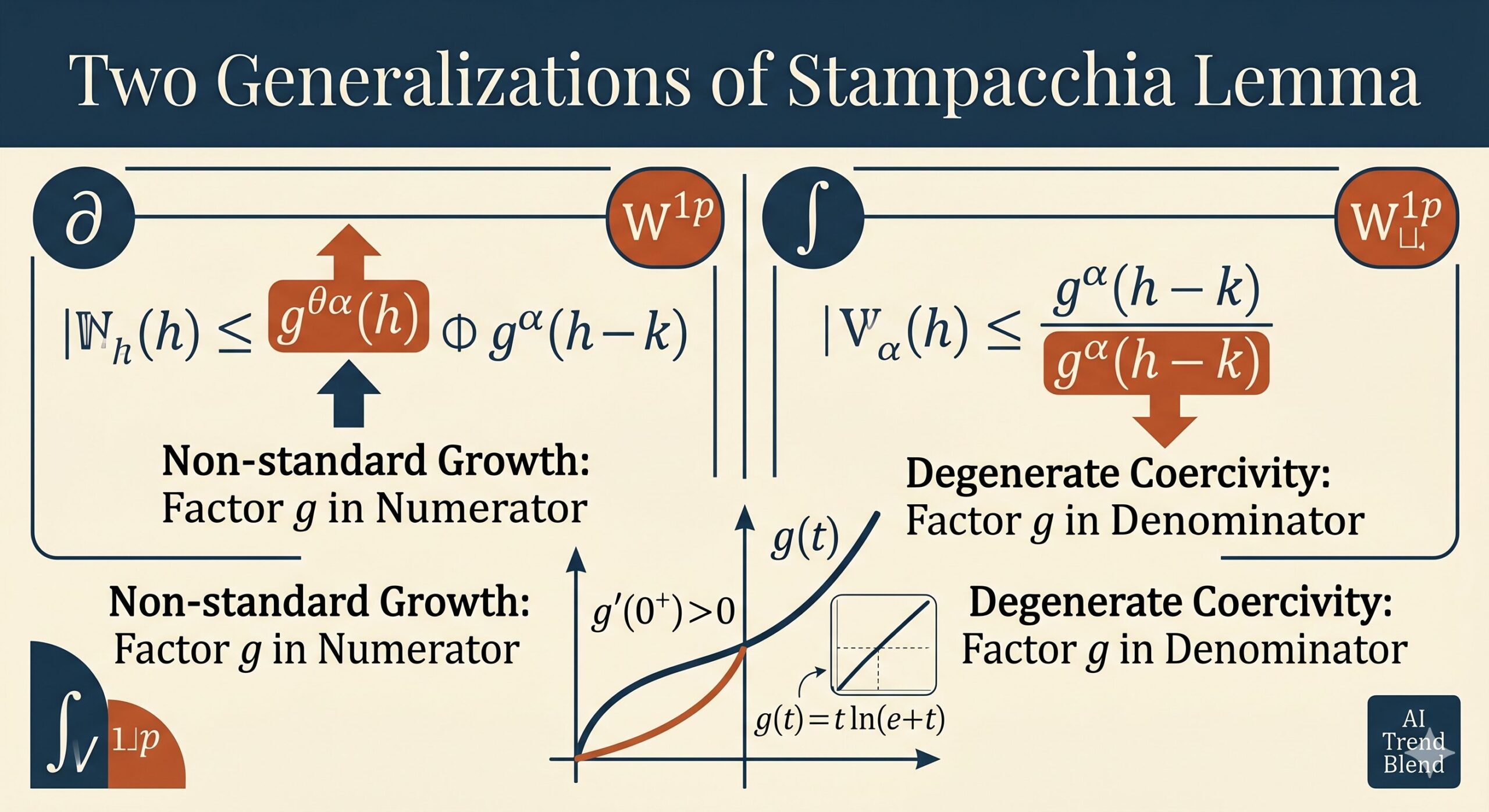
Stampacchia Lemma Elliptic PDEs Regularity Theory Nonstandard Growth Variational Integrals Degenerate Elliptic Marcinkiewicz Spaces De Giorgi Technique

The Stampacchia Lemma, sometimes called the De Giorgi–Stampacchia Lemma, is one of those results that appears again and again whenever analysts want to prove that solutions of elliptic equations are bounded or that minimizers of variational integrals have higher integrability than the problem’s basic setup guarantees. The classical version is elegant but limited. This paper extends it twice — once to handle a function g hiding in the denominator, and once to handle g appearing in the numerator — and applies both extensions to real problems where the classical lemma simply cannot reach.

Why the Classical Lemma Is Both Powerful and Limiting

To appreciate what this paper does, it helps to understand what the original Stampacchia Lemma actually says, and why analysts keep needing to push it further.

The lemma starts with a non-increasing function $\phi : [k_0, +\infty) \to [0, +\infty)$ — think of it as measuring the “size” of the set where a solution exceeds a given threshold $k$. If you can show that this function satisfies an inequality of the form

Classical Stampacchia $$\phi(h) \leq \frac{c}{(h-k)^\alpha} [\phi(k)]^\beta$$

for all $h > k \geq k_0$, then depending on whether $\beta > 1$, $\beta = 1$, or $0 < \beta < 1$, you get three qualitatively different conclusions about how fast $\phi$ decays. The most powerful case, $\beta > 1$, gives you finite vanishing: $\phi(2L) = 0$ for a computable $L$, which translates directly into $L^\infty$ boundedness for solutions.

The problem appears as soon as you try to apply this to equations or functionals where the coercivity degenerates. Consider, for example, a variational integral with integrand satisfying

Nonstandard Growth $$\nu |z|^p \ln^p(e + |z|) + a(x) \leq f(x, z)$$

or an elliptic equation where the coefficient satisfies

Degenerate Coefficient $$\frac{\alpha}{(1+|s|)^\theta \ln^\theta(e+|s|)} \leq a(x,s) \leq \beta, \quad 0 \leq \theta < 1$$

These are legitimate, naturally occurring conditions in mathematical physics — but when you try to derive the Stampacchia-type inequality from them, you end up with something like

New Form Needed $$\phi(h) \leq \frac{c\, h^{\theta\alpha}}{g^\alpha(h-k)} [\phi(k)]^\beta \quad \text{or} \quad \phi(h) \leq \frac{c\, g^{\theta\alpha}(h)}{(h-k)^\alpha} [\phi(k)]^\beta$$

where $g(t) = t\ln(e+t)$ or some similarly structured function. The classical lemma does not cover either of these forms. The previous extension by Gao, Zhang and Ma handled a factor $h^{\theta\alpha}$ in the numerator but not a $g^\alpha$ in the denominator. This paper fills both gaps simultaneously.

The Core Insight

Both generalizations replace a pure power $(h-k)^\alpha$ or $h^{\theta\alpha}$ with expressions involving a non-decreasing function $g$ satisfying three conditions: convexity and positivity, a sub-power growth bound $g(\lambda t) \leq \lambda^\mu g(t)$, and a positive derivative at zero. The prototype is $g(t) = t\ln(e+t)$, which grows slightly faster than a pure power but not as fast as an exponential. This mild extra growth is exactly what logarithmic nonstandard conditions produce.

The Function g — What It Is and Why It Works

The authors are careful to define their function class precisely, because the entire analysis depends on three properties of $g$. Let $g : [0,+\infty) \to [0,+\infty)$ satisfy the following:

(G1) $g$ is $C^1$, convex, and non-decreasing, with $g(0) = 0$ and $g(t) > 0$ for all $t > 0$.
(G2) There exists a constant $\mu \geq 1$ such that $g(\lambda t) \leq \lambda^\mu g(t)$ for every $\lambda > 1$ and every $t > 0$. This is a sub-power growth condition — $g$ cannot grow faster than a polynomial in its argument.
(G3) The one-sided derivative at zero satisfies $g'(0^+) > 0$.

The canonical example is $g(t) = t\ln(e+t)$. This function is smooth, convex, strictly positive for $t > 0$, satisfies $g(\lambda t) \leq \lambda^2 g(t)$ for all $\lambda > 1$ and $t > 0$ (so $\mu = 2$), and clearly has $g'(0^+) = 1 > 0$. It is precisely the function that appears in logarithmic nonstandard growth conditions, which is why this paper’s applications land exactly where they should.

Two lemmas about $g$ underpin everything that follows. The first says that for any $t \geq 0$, we have $g'(t) t \leq \mu g(t)$ — a relationship between the derivative and the function itself that comes directly from the sub-power growth condition. The second says that for any $t_1, t_2 \geq 0$, we have $g'(t_1) t_2 \leq g'(t_1) t_1 + g'(t_2) t_2$. This second inequality is a consequence of the monotonicity of $g’$, which follows from convexity, and it is used repeatedly in the application to variational integrals when estimating cross terms involving the gradient.

The First Generalization — g in the Denominator

The first main result, Theorem 2.1, covers the case where the function $g$ appears in the denominator of the bounding inequality:

First Generalization $$\phi(h) \leq \frac{c\, h^{\theta\alpha}}{g^\alpha(h-k)} [\phi(k)]^\beta, \quad \forall h > k \geq k_0 > 0$$

Here $0 \leq \theta < 1$ must satisfy an additional decay condition: $\lim_{L \to \infty} L^\theta / g(L) = 0$, which ensures that $L^\theta$ grows strictly slower than $g(L)$. For $g(t) = t\ln(e+t)$, this condition holds even for $\theta = 1$, because $L / (L\ln(e+L)) \to 0$.

The theorem delivers three conclusions, one for each regime of $\beta$:

Theorem 2.1 — Three Regimes

Case $\beta > 1$: There exists an explicit $L$ satisfying $L \geq 2k_0$ and a condition on $g(L)/L^\theta$ such that $\phi(2L) = 0$. The level $L$ is determined by balancing $c^{1/\alpha}[\phi(k_0)]^{(\beta-1)/\alpha}$ against a power of 2 depending on $\mu$, $\beta$, and $\theta$. This gives finite $L^\infty$ bounds for solutions.

Case $\beta = 1$: For any $k \geq k_0$, the function $\phi$ decays sub-exponentially: $\phi(k) \leq \phi(k_0) \exp\!\bigl(1 – ((k-k_0)/\tilde\tau)^{1-\theta}\bigr)$ for a computable $\tilde\tau$. This is weaker than pure exponential decay but still gives exponential integrability of the solution.

Case $0 < \beta < 1$: The decay is algebraic in $g(k)$: $\phi(k) \leq C (1/g(k))^{\alpha(1-\theta)/(1-\beta)}$, which translates into Marcinkiewicz-space membership for the solution with an exponent higher than the Sobolev exponent.

The proof strategy is the same in all three cases, following the De Giorgi iteration approach: choose a geometric sequence of levels $t_i = 2L(1 – 2^{-i-1})$, plug consecutive pairs into the assumed inequality, and use the sub-power growth condition (G2) to bound $g^\alpha(L \cdot 2^{-i-1})$ in terms of $g^\alpha(L)$. This converts the original inequality into one of the form $x_{i+1} \leq C B^i x_i^\beta$, to which a standard iteration lemma applies.

What makes the proof work is that condition (G2) gives $g(L) \leq 2^{(i+1)\mu} g(L \cdot 2^{-i-1})$, so the factor of $g$ in the denominator can be controlled uniformly across all levels in the sequence. This is where the sub-power growth of $g$ is essential — an exponentially growing function would not allow this estimate.

“The factor $g^\alpha$ in the denominator of the bounding inequality cannot be handled by the classical argument or by previous extensions involving pure powers. The key is condition (G2): sub-power growth ensures that $g$ evaluated along the geometric level sequence stays comparable to $g$ at the initial level, allowing the standard iteration to proceed.” — Han, Fang, Xia, Gao, Gao · J. Math. Anal. Appl. 563 (2026)

One particularly useful corollary arises when $\theta = 0$, reducing the bounding inequality to

Corollary 2.1 (θ = 0) $$\phi(h) \leq \frac{c}{g^\alpha(h-k)} [\phi(k)]^\beta$$

and producing cleaner formulas for $L$, $\tilde\tau$, and the algebraic decay rate. This corollary is used directly in the application to variational integrals.

When Are the Full Assumption and the Doubled Version Equivalent?

Before moving on, the paper resolves a subtle question: is the full assumption (requiring the bound for all $h > k$) equivalent to the simpler doubled assumption $\phi(2k) \leq c/g^\alpha(k) [\phi(k)]^\beta$ obtained by just setting $h = 2k$? The answer depends on $\beta$.

Case 0 < β < 1 — Equivalent

Theorem 2.2 shows these two conditions are equivalent when $0 < \beta < 1$. You can work with either form; the doubled version is often easier to verify from estimates on solutions.

Cases β ≥ 1 — Not Equivalent

Theorems 2.3 and 2.4 give explicit counterexamples for $\beta = 1$ and $\beta > 1$: functions that satisfy the doubled version but not the full assumption. So for these cases, you genuinely need to verify the full inequality.

The counterexample for $\beta = 1$ is the function $\phi(k) = e^{-(\ln k)^2}$, which satisfies the doubled inequality with $g(k) = k^2 + k$ and $\alpha = \ln 2$, but cannot satisfy the full inequality with $\beta = 1$ for any choice of $c$, $\alpha$, and $g$ — because the full inequality would force sub-exponential decay, but $e^{-(\ln k)^2}$ decays much more slowly than any exponential.

Application to Variational Integrals with Log-Power Growth

The first generalization’s main application is to variational integrals of the form

Variational Integral $$\mathcal{J}(u;\Omega) = \int_\Omega f(x, Du(x))\, dx$$

where the integrand $f$ satisfies the log-power lower bound $\nu g^p(|z|) – a(x) \leq f(x,z)$ with $g(t) = t\ln(e+t)$. This is the key nonstandard growth condition: the integrand grows like $|z|^p \ln^p(e+|z|)$ from below, which is slightly faster than a pure $p$-th power but not as fast as a $(p+\varepsilon)$-th power. Previous regularity results handled pure power growth; this paper handles the logarithmically corrected case.

The main result, Theorem 2.5, assumes that the boundary datum $u^*$ and the auxiliary function $a(x)$ belong to $L^\sigma(\Omega)$ for some $\sigma > 1$, and then derives:

If $\sigma > n/p$: the difference $u – u^*$ is essentially bounded — $u – u^* \in L^\infty(\Omega)$.
If $\sigma = n/p$: there exists $\tau > 0$ depending on the data such that $e^{\tau|u-u^*|} \in L^1(\Omega)$ — exponential integrability at the critical exponent.
If $\sigma < n/p$: the function $g(|u-u^*|) = |u-u^*|\ln(e+|u-u^*|)$ belongs to the Marcinkiewicz space $L^{np\sigma/(n-p\sigma)}_w(\Omega)$ — weak-type integrability with an exponent above the standard Sobolev exponent $p^* = np/(n-p)$.

The proof is a careful combination of three ingredients. First, the minimality of $u$ is used to compare $\mathcal{J}(u;\Omega)$ with $\mathcal{J}(w;\Omega)$ for a carefully chosen competitor function $w = u – G_k(u-u^*)$, where $G_k$ is the truncation above level $k$. This gives an integral inequality controlling the gradient of $u – u^*$ over the superlevel set $A_k = \{|u-u^*| > k\}$. Second, the Sobolev inequality is applied to the function $g((|u-u^*|-k)_+)$ — and here the sub-power growth condition on $g$ is essential for showing that this function actually lies in $W^{1,p}_0(\Omega)$. Third, the resulting inequality is identified as an instance of Corollary 2.1, and the three cases of the lemma give the three conclusions of the theorem.

Why This Matters

In the special case $g(t) = t$ (pure power growth), Theorem 2.5 reduces exactly to the result of Leonetti and Petricca from 2015. The new theorem covers all functions $g$ satisfying (G1)–(G3), which includes $g(t) = t\ln(e+t)$, $g(t) = t\ln^2(e+t)$, and other log-corrected growth functions. This is the natural class for modern regularity theory with borderline growth conditions.

The Second Generalization — g in the Numerator

The second main result, Lemma 3.1, handles the complementary situation where $g$ appears in the numerator:

Second Generalization $$\phi(h) \leq \frac{c\, g^{\theta\alpha}(h)}{(h-k)^\alpha} [\phi(k)]^\beta, \quad \forall h > k \geq k_0 > 0$$

This form arises naturally from elliptic equations where the coefficient $a(x,s)$ involves a degeneracy like $(1+|s|)^{-\theta}\ln^{-\theta}(e+|s|)$. When you estimate the superlevel sets via the Sobolev inequality, the factor $(1+h)^\theta \ln^\theta(e+h)$ from the coefficient ends up in the numerator of the Stampacchia-type inequality, giving exactly the form above with $g(t) = t\ln(e+t)$.

The conclusions follow the same three-case structure, but the conditions are somewhat more delicate:

Lemma 3.1 — Three Cases

Case $\beta > 1$, $\theta < 1$: Requires $\lim_{L\to\infty} g^\theta(L)/L = 0$, which is satisfied by $g(t) = t\ln(e+t)$ for any $\theta < 1$. Gives $\phi(2L) = 0$ for a computable $L$.

Case $\beta = 1$, $\mu\theta < 1$: Requires the existence of $\tilde\theta > \theta$ with $\lim_{L\to\infty} g^{\tilde\theta}(L)/L = 0$. The decay rate is sub-exponential with exponent $1 – \theta/\tilde\theta$. The condition $\mu\theta < 1$ is a smallness condition on $\theta$ relative to the sub-power growth exponent $\mu$.

Case $0 < \beta < 1$, $\theta < 1$: Requires the existence of $\varepsilon_0 \in (0, 1-\theta)$ such that $g'(k)/g^{1-\theta-\varepsilon_0}(k) \to 0$ as $k \to \infty$. This is a mild regularity condition on $g$, satisfied by $g(t) = t\ln(e+t)$ for any $\varepsilon_0 < 1-\theta$. Gives algebraic decay in $g(k)$ with exponent $\varepsilon_0\alpha/(1-\beta)$.

The proof for the $\beta > 1$ case is analogous to the first generalization, using condition (G2) to bound $g^\theta(2L)$ in terms of $g^\theta(L)$. For the $\beta = 1$ case, the argument is more involved: the key is to choose a sequence of levels $k_s = k_0 + \tau s^{\tilde\theta/(\tilde\theta – \theta)}$ (growing faster than linearly), apply the Taylor expansion to bound the step sizes $k_{s+1} – k_s$ from below, and use the Mean Value Theorem for $g$ to convert the factor $g^\theta(h)$ into something involving $g'(0^+)$. The resulting inequality contracts by a factor of at most $1/e$ at each level, giving the claimed sub-exponential decay.

Special Case: g(t) = t ln(e + t)

Corollary 3.1 specializes Lemma 3.1 to the specific function $g(t) = t\ln(e+t)$, giving explicit conditions for each case. For instance, the $\beta > 1$ case requires $\ln^\theta(e+L)/L^{1-\theta}$ to be small, which holds for large $L$ since $L^{1-\theta}$ grows faster than any logarithm. The $\beta < 1$ case gives a clean decay bound involving $(1/g(k))^{\varepsilon_0\alpha/(1-\beta)} = (1/(k\ln(e+k)))^{\varepsilon_0\alpha/(1-\beta)}$.

Application to Degenerate Elliptic Equations

The second generalization’s application is to the degenerate elliptic boundary value problem

Degenerate Elliptic BVP $$-\text{div}(a(x, u(x)) Du(x)) = f(x) \text{ in } \Omega, \quad u = 0 \text{ on } \partial\Omega$$

where the coefficient satisfies the logarithmically degenerate ellipticity condition

Log-Degenerate Coefficient $$\frac{\alpha}{(1+|s|)^\theta \ln^\theta(e+|s|)} \leq a(x,s) \leq \beta, \quad 0 \leq \theta < 1$$

and the right-hand side $f$ belongs to the Marcinkiewicz space $L^m_w(\Omega)$ for some $m > (2^*)’ = 2n/(n+2)$. This problem is not coercive on $W^{1,2}_0(\Omega)$ in the usual sense because the lower bound on $a$ degenerates when $|s|$ is large. Existence results for this type of problem were proved by Boccardo, Dall’Aglio, and Orsina for the simpler case $a(x,s) \geq \alpha/(1+|s|)^\theta$; the present paper handles the additional logarithmic factor.

Theorem 3.1 proves that if $u \in W^{1,2}_0(\Omega)$ is a weak solution, then:

When $m > n/2$ and $0 \leq \theta < 1$: the solution is bounded, $|u| \leq 2L$ for a computable $L$.
When $m = n/2$ and $\mu\theta < 1$: for any $\rho < 1-\theta$, there exists $\lambda > 0$ such that $e^{\lambda|u|^\rho} \in L^1(\Omega)$ — stretched exponential integrability at the critical exponent.
When $(2^*)’ < m < n/2$ and $0 \leq \theta < 1$: the function $|u|\ln(e+|u|)$ belongs to $L^\varrho_w(\Omega)$ for any $\varrho < m^{**}(1-\theta)$, where $m^{**} = nm/(n-2m)$ is the double Sobolev exponent.

The proof reduces everything to verifying that the superlevel sets $A_k = \{|u| > k\}$ satisfy an inequality of the form covered by Corollary 3.1. This is done by testing the weak formulation with $T_{h-k}(G_k(u))$ — a standard De Giorgi test function — and estimating both sides using the Sobolev inequality and the Hölder inequality for Marcinkiewicz spaces. The logarithmic degeneracy in $a$ produces the factor $(1+h)^\theta\ln^\theta(e+h)$ in the numerator of the resulting estimate, which is precisely what Corollary 3.1 handles.

The Technical Point That Makes It Work

Testing the weak equation with $T_{h-k}(G_k(u))$ and using the degenerate ellipticity condition produces an estimate where the Sobolev inequality on the left gives a factor of $(h-k)^{2^*/2}$ in the denominator, while the right side contributes $(1+h)^{\theta \cdot 2^*/2}\ln^{\theta \cdot 2^*/2}(e+h)$ from the coefficient. Setting $g(t) = t\ln(e+t)$, this is exactly $g^{\theta \cdot 2^*/2}(1+h) / (h-k)^{2^*/2} \cdot [\phi(k)]^{2^*/(2m’)}$, which matches the form of Corollary 3.1 with $\alpha = 2^*/2$ and $\beta = 2^*/(2m’)$.

What These Results Mean for PDE Regularity Theory

Taken together, the two generalizations in this paper significantly expand the toolkit available for proving regularity results for problems with nonstandard growth. The classical Stampacchia Lemma and its previous extensions handled polynomial-type degeneracies and growth conditions. The new versions handle growth conditions that involve logarithmic corrections — precisely the borderline cases that sit between different Sobolev exponents and often require the most care.

Several features of the paper are worth noting from a methodological perspective:

First, the function class for $g$ is explicit and flexible. The three conditions (G1)–(G3) are easy to verify for concrete functions, and the sub-power growth condition (G2) is the key constraint — it is weak enough to include interesting examples like $g(t) = t\ln(e+t)$ but strong enough to make the iteration argument work.

Second, the paper carefully distinguishes which case of $\beta$ needs the full strength of the lemma versus which can get by with the doubled version. For $0 < \beta < 1$, the doubled version suffices; for $\beta \geq 1$, it does not. This matters for applications because the doubled version is often what you can directly read off from an integral estimate.

Third, the applications to variational integrals and elliptic equations are genuine rather than artificial — the logarithmic nonstandard growth conditions in the paper correspond to real mathematical objects that arise in the study of fluids, elasticity, and other physical models where the constitutive relations involve mild logarithmic corrections to power-law behavior.

Fourth, in the critical exponent case $\sigma = n/p$ for variational integrals (or $m = n/2$ for the elliptic equation), the paper obtains exponential integrability of the solution rather than mere boundedness. This is the correct sharp result at the critical Sobolev exponent — exponential integrability is the best one can hope for without the strict inequality $\sigma > n/p$.

The Full Structure at a Glance

To summarize the paper’s logical architecture: two generalized lemmas are proved — one with $g$ in the denominator, one with $g$ in the numerator. Each lemma has three cases depending on $\beta$. For the first lemma, the equivalence between the full assumption and the doubled version is characterized precisely. Each lemma is then applied to a concrete PDE or variational problem with the specific function $g(t) = t\ln(e+t)$, recovering and extending previous regularity results in a unified framework.

The paper builds directly on earlier work by Gao and collaborators — the 2020 regularity paper for entropy solutions, the 2021 paper on quasilinear elliptic systems, the 2026 paper on a further Stampacchia generalization — while also engaging with the classical Italian school results of Boccardo, Dall’Aglio, Orsina, and the Sobolev embedding techniques of Cupini, Marcellini, and Mascolo. The result is a coherent contribution that closes a gap in the existing theory without requiring fundamentally new proof techniques — instead, it shows how careful formulation of the function class $g$ allows the existing De Giorgi iteration machinery to be pushed into logarithmic territory.

Read the Full Paper

Published open access in the Journal of Mathematical Analysis and Applications under CC BY 4.0. All proofs, lemmas, corollaries, and full bibliographic details are freely available.

📄 Read the Paper (DOI) 🔗 JMAA Journal Page

Academic Citation:
Han Yingxiao, Fang Mi, Xia Liuye, Gao Hongya, Gao Siyu. Two generalizations of Stampacchia lemma and applications. Journal of Mathematical Analysis and Applications, 563 (2026) 130734. https://doi.org/10.1016/j.jmaa.2026.130734

This article is an independent editorial analysis of a peer-reviewed open-access paper. Mathematical statements paraphrase the original results; for precise formulations and complete proofs, refer to the published paper. The fourth author (Gao Hongya) acknowledges support from the NSF of Hebei Province, Grant No. A2024201024.

References

[1] L. Boccardo, The summability of solutions to variational problems since Guido Stampacchia. Rev. R. Acad. Cienc. 97(3) (2003) 413–421.
[2] L. Boccardo, G. Croce, Elliptic Partial Differential Equations. De Gruyter Studies in Mathematics, vol. 55, 2014.
[3] L. Boccardo, A. Dall’Aglio, L. Orsina, Existence and regularity results for some elliptic equations with degenerate coercivity. Atti Semin. Mat. Fis. Univ. Modena 46 (1998) 51–81.
[4–6] G. Cupini, P. Marcellini, E. Mascolo, Regularity under sharp anisotropic general growth conditions; Local boundedness of minimizers with limit growth conditions; Regularity of minimizers under limit growth conditions. Discrete Contin. Dyn. Syst. B (2009); J. Optim. Theory Appl. (2015); Nonlinear Anal. (2017).
[7] H. Gao, H. Deng, M. Huang, W. Ren, Generalizations of Stampacchia lemma and applications to quasilinear elliptic systems. Nonlinear Anal. 208 (2021) 112297.
[8] H. Gao, M. Huang, W. Ren, Regularity for entropy solutions to degenerate elliptic equations. J. Math. Anal. Appl. 491 (2020) 124251.
[9] H. Gao, J. Zhang, H. Ma, A generalization of Stampacchia lemma and applications. J. Convex Anal. 33 (2026) 1–12.
[12] E. Giusti, Direct Methods in the Calculus of Variations. World Scientific, 2003.
[15] F. Leonetti, P.V. Petricca, Regularity for minimizers of integrals with non standard growth. Nonlinear Anal. 129 (2015) 258–264.
[17] G. Stampacchia, Équations elliptiques du second ordre á coefficients discontinus. Séminaire Jean Leray, vol. 3, 1963.