Liquid Biopsy and AI: Multi-Cancer Early Detection — 10 Claude Code Prompts for MCED Research (2026)
Multi-Cancer Early Detection
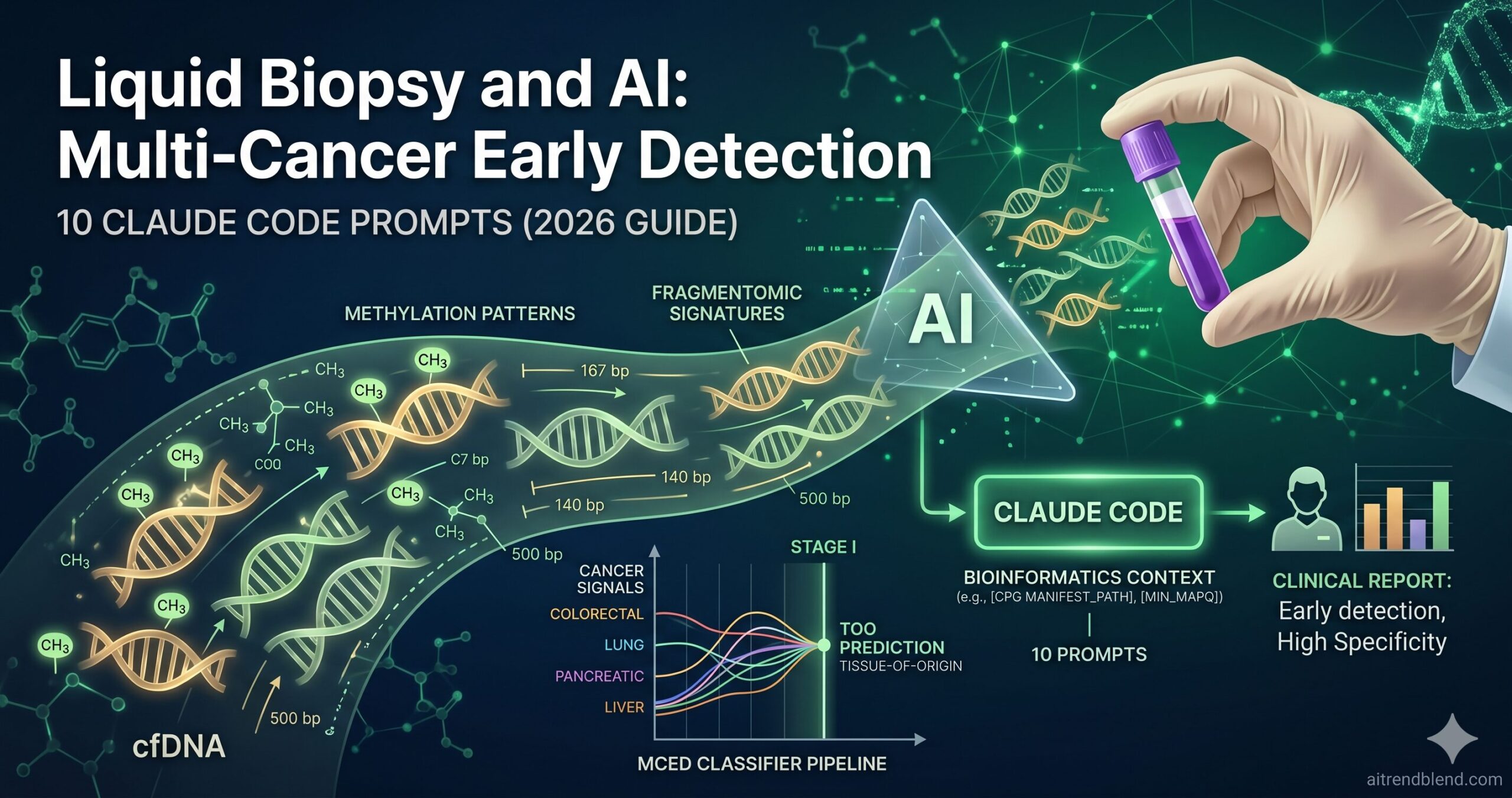
Liquid biopsy for multi-cancer early detection is one of the most consequential diagnostic innovations of the past decade — and one of the most computationally demanding. The signal you’re looking for is vanishingly small: at Stage I, circulating tumour DNA (ctDNA) may constitute less than 0.01% of all cell-free DNA in a blood sample. Finding it reliably, distinguishing it from biological noise, predicting which tissue it came from, and doing this simultaneously for twenty different cancer types — that is not a sensitivity problem any single biomarker solves. It requires machine learning that integrates DNA methylation patterns, fragment size distributions, end-motif signatures, and protein biomarkers into a unified cancer signal classifier.
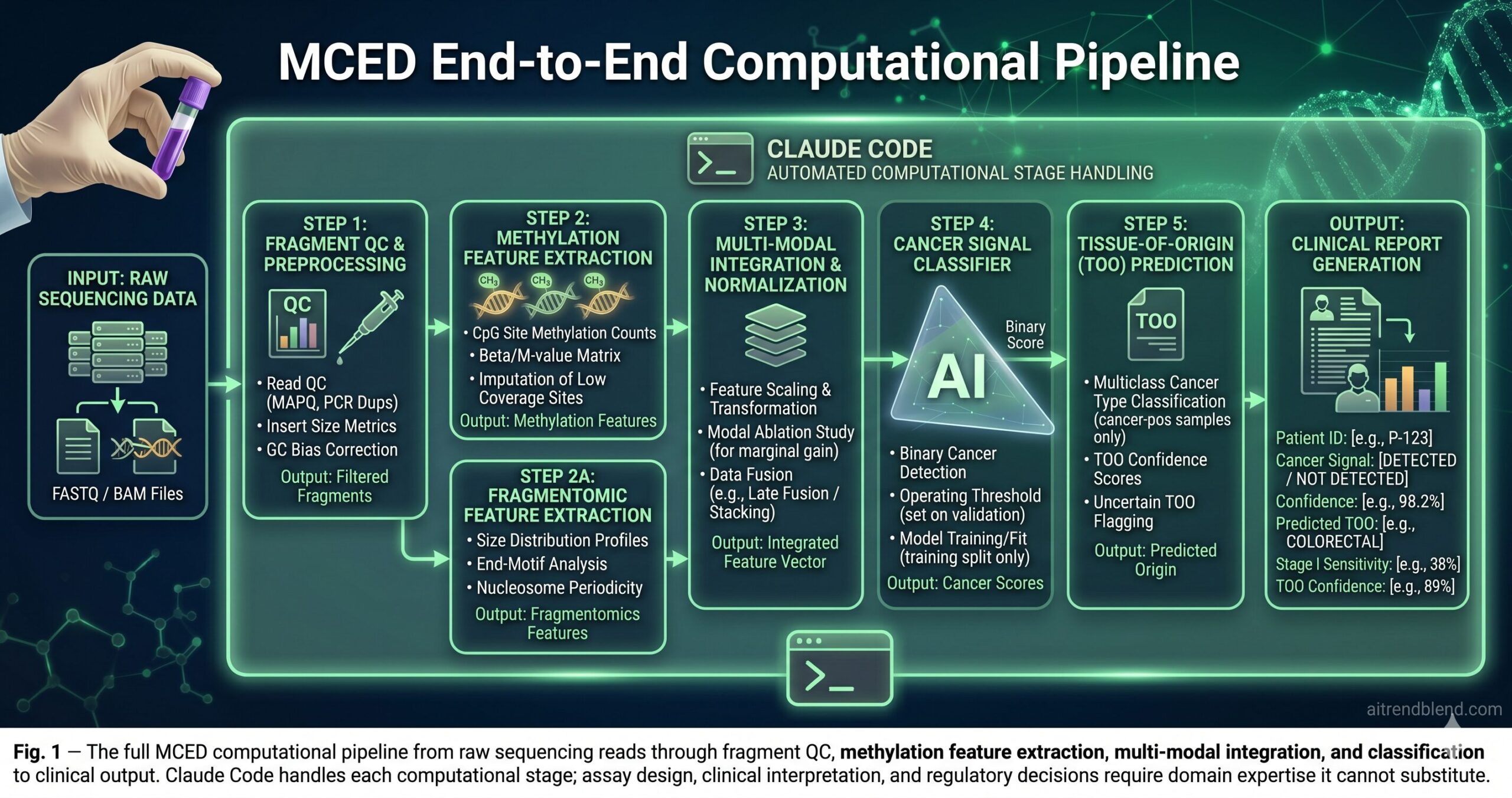
AI researchers and bioinformaticians building these pipelines face the same challenge as any high-stakes ML practitioner: the gap between code that runs and code that produces clinically reliable results is wide and not always visible until peer review. Claude Code — operating inside your project with full context of your sequencing parameters, your existing bioinformatics utilities, and your data schema — closes that gap faster than any chat-interface approach. The prompts in this guide cover the full MCED research pipeline, from raw fragment-level data processing to the clinical validation frameworks that FDA reviewers and journal editors actually examine.
This is not a beginner’s introduction to liquid biopsy. It is a working guide for computational biologists, bioinformaticians, and AI engineers who already understand the domain and want to move faster and more reliably within it. The science is not simplified. The prompts are not generic. Each one is designed around a specific failure mode in MCED research that affects published results and clinical translation.
Why Claude Code Handles MCED Research Differently
The problem most bioinformaticians run into with general AI tools is that genomics pipelines have domain-specific complexity that generic code generation doesn’t model. A tool that treats a BED file and a BAM file as interchangeable inputs, generates methylation feature code without understanding why CpG methylation patterns differ between cancer types and healthy tissue, or produces a training loop without enforcing the train/test split required to prevent data leakage — that tool generates plausible-looking code that requires as much expert correction as writing it from scratch.
Claude Code’s project-wide context changes what’s possible. Point it at your preprocessing scripts, your reference genome configuration, your existing feature extraction utilities, your training data schema — and the code it generates reflects the actual architecture of your pipeline. For MCED research specifically, this means it uses your CpG site coordinates, your sequencer-specific quality thresholds, your tissue-of-origin label schema, and your existing model evaluation framework. The generated code fits into your pipeline rather than requiring adaptation before it runs.
Commercial MCED development tools handle standardised workflows well for labs running established assay formats. Bioinformatics platforms like Nextflow and Snakemake are excellent for workflow orchestration. Claude Code occupies a different role: it is the tool you use when you need to build or substantially modify the analytical logic — the classifier architecture, the feature engineering design, the multi-modal integration approach — and when scaffold code from a chat interface would require more expert correction than it saves. For research groups developing novel MCED methods, that’s where the real work lives.
MCED pipelines fail in bioinformatics-specific ways — incorrect fragment coordinate handling, data leakage across cancer type splits, inappropriate normalisation for low-coverage sequencing, and sensitivity estimates that ignore stage distribution. Claude Code’s project context surfaces these as code review issues rather than silent analysis errors that persist into publication.
Why AI Is Reshaping Multi-Cancer Early Detection
Traditional cancer screening works organ by organ — mammography for breast, PSA for prostate, colonoscopy for colorectal. Each test is optimised for one cancer type. Multi-cancer early detection inverts this entirely: a single blood draw, a single assay, a single classifier that must simultaneously detect signals from over twenty cancer types — many of which have no established screening test at all. Pancreatic cancer, ovarian cancer, oesophageal cancer. These are found late not because they grow slowly, but because there has been no practical way to find them early. That is the problem liquid biopsy AI is attempting to solve.
The signal source is cell-free DNA (cfDNA): short double-stranded fragments released into the bloodstream when cells die through apoptosis or necrosis. In healthy individuals, cfDNA comes predominantly from haematopoietic cells. In cancer patients, a fraction comes from tumour cells — this cancer-derived subset is circulating tumour DNA (ctDNA). At Stage I, the variant allele frequency (VAF) — the proportion of cfDNA carrying a tumour-derived signal — can be below 0.1%. Standard sequencing at conventional depth cannot reliably detect signals this faint above the sequencing error floor.
Here is where it gets interesting. DNA methylation patterns are highly tissue-specific and are preserved in the cfDNA fragments those cells shed. The same CpG locus may be methylated in hepatocytes and unmethylated in colonocytes. Machine learning classifiers trained on hundreds of thousands of CpG methylation sites can learn to distinguish tumour-derived methylation patterns from healthy tissue cfDNA — and to identify which tissue type the signal is most likely coming from. This tissue-of-origin (TOO) prediction capability transforms a binary positive/negative result into an actionable clinical signal: “colorectal cancer signal detected, Stage I, high confidence.” That is qualitatively different from “something may be abnormal.”
None of this is a solved problem. Stage I sensitivity for most cancers in leading MCED tests ranges from 20% to 45% as of 2026. The specificity required for population screening — where 99% of tested individuals have no cancer — means even a 1% false positive rate generates ten false alarms for every true positive in a typical low-prevalence screening population. Knowing these constraints is not pessimism; it is the foundation for building AI systems that handle them correctly rather than obscuring them in headline accuracy numbers.
MCED AI is not about maximising accuracy on a balanced dataset. It is about maintaining extremely high specificity — 99.5% or higher for population screening — while maximising stage-stratified sensitivity, especially at Stage I and Stage II where curative treatment is most available. Any classifier that omits realistic population prevalence from its performance reporting is not ready for clinical translation.
Before You Start: How to Get the Best Results
MCED research pipelines have technical and regulatory complexity that shapes every prompt you write. These foundations are worth establishing once, carefully, before any computational work begins.
Document your sequencing parameters in CLAUDE.md before any session. Target sequencing depth, read length, library preparation method — bisulfite conversion for methylation, cfDNA-optimised prep for fragmentomics — reference genome build, and the coordinate system for your CpG site manifest. A methylation feature extraction script designed for 30× WGBS data will not work correctly on 0.3× WGBS data without fundamental model changes. Claude Code generates the right code for your parameters when those parameters are explicitly in its context.
Maintain a documented, version-controlled train/validation/test split protocol and reference it in every prompt that touches model training or evaluation. In MCED research, the temptation to evaluate on data used for feature selection is real because sample collection is expensive. This is the most common source of inflated performance metrics in published MCED studies. Your split file should be treated as an immutable artefact — created once from the full cohort, never modified, explicitly cited in every evaluation prompt.
Keep your cancer type label schema as a structured reference file. MCED pipelines typically handle 10 to 25 cancer types plus healthy controls. Inconsistency between the label schema used in training and the one used in evaluation is a silent source of misclassification that only surfaces in detailed per-class confusion analysis — often after reviewers ask why certain cancer type accuracies look anomalous.
The 10 Best Claude Code Prompts for Liquid Biopsy and MCED Research
These prompts run in a terminal with claude active in your bioinformatics project directory. Amber variables are yours to fill before running. Complexity escalates from fragment-level data processing to the clinical validation and regulatory documentation frameworks that MCED translation requires.
Prompt 1: The cfDNA Fragment Length Profiler
Fragment length distribution is the first signal worth characterising in any cfDNA dataset. Healthy cfDNA shows a mononucleosomal peak around 167 bp, reflecting nucleosome-protected DNA. Tumour-derived cfDNA — from proliferating cells with altered chromatin architecture — shows relative enrichment of short fragments below 150 bp and a shifted peak position. Quantifying this shift is the foundation of fragmentomics-based detection, and it starts with a rigorously GC-corrected fragment size profile.
The GC-content LOESS correction is the step that separates a reliable fragment profiler from one that produces false cancer signals. Short-fragment enrichment is confounded by GC bias introduced during library preparation — high-GC regions produce shorter apparent fragments in some sequencing chemistries. Without this correction, SFR elevations that look like tumour signal are frequently sequencing batch effects. Embedding the correction as a required computational step, using your actual control samples, prevents this artefact from propagating into downstream classifiers where it would silently inflate sensitivity estimates.
Add “Compute fragment size profiles restricted to genomic regions with high differential chromatin accessibility in cancer vs. normal tissue using the ATAC-seq reference atlas at [ATLAS_PATH]” — these locus-specific fragment features have substantially stronger discriminative power than genome-wide averages for most cancer types.
Prompt 2: The Methylation Feature Extractor
DNA methylation at CpG sites is the most information-rich signal in cfDNA-based cancer detection. The methylation state of hundreds of thousands of CpG sites varies systematically between cancer types and healthy tissue — and that pattern is preserved in cfDNA fragments. Extracting clean, well-normalised methylation features from bisulfite-converted sequencing data is technically demanding. Conversion efficiency, coverage depth, and CpG site selection all affect downstream classifier performance in ways that aggregate validation metrics obscure.
The bisulfite conversion efficiency gate — using CpH methylation rate as a proxy for incomplete conversion — is the quality check that prevents corrupted samples from entering the feature matrix. Failed conversion produces genome-wide apparent hypomethylation: beta values shift systematically downward in a pattern that the classifier will learn to associate with signal rather than noise. By raising an error rather than imputing over a failed conversion, the pipeline protects the integrity of every downstream model trained on that feature matrix.
Add “Compute methylation haplotype block (MHB) linkage statistics — co-methylation across consecutive CpG sites on the same fragment — and include phased methylation patterns as additional features” to capture epigenetic heterogeneity signals that single-CpG beta values systematically miss.
Prompt 3: The Cancer Signal Binary Classifier
The first classification problem in MCED is binary: is there a detectable cancer signal in this sample? Before tissue-of-origin prediction, before stage estimation, the system determines whether any ctDNA signal is present above the noise floor. This classifier sets the specificity of the entire assay. For population screening, that specificity must be calibrated to the actual population prevalence — not the balanced or enriched cohort used for training.
The number-needed-to-screen and false-positives-per-10,000 metrics are what translate classifier performance into clinical decision-making language. A senior clinician or payer reviewing an MCED assay does not think in AUC units — they think in terms of how many unnecessary follow-up procedures a positive result triggers for every true cancer found. Building these calculations into every evaluation report ensures performance is communicated in the terms that actually govern clinical adoption decisions.
Add “Compute sensitivity as a function of ctDNA VAF using samples with measured tumour fraction” to characterise the minimum detectable tumour burden — the most clinically important performance parameter for early-stage detection that aggregate AUC metrics never reveal.
Prompt 4: The Tissue-of-Origin Prediction Module
Most tutorials skip this part entirely. Tissue-of-origin prediction — determining which organ the cancer signal is most likely coming from — is what transforms a binary detection result into an actionable clinical finding. A positive signal without TOO guidance tells a clinician only that something may be wrong. A positive signal with 89% confidence for colorectal origin, confirmed by colonoscopy seven days later at Stage II — that is the clinical value proposition of MCED. Building a reliable TOO classifier across 20+ cancer types requires handling class imbalance, prediction uncertainty, and calibration with precision.
The “train on cancer-positive samples ONLY” instruction prevents the most common architecture error in TOO classifier design. A TOO model that sees healthy controls during training learns a spurious “no cancer” class — a class it should never encounter, because the TOO module only receives samples already classified as cancer-positive by the binary detector. Including healthy controls in TOO training contaminates the decision boundary and produces overconfident predictions that fail when the two-stage pipeline runs in sequence.
Add “Evaluate whether a hierarchical TOO design — first predict broad category (GI/GYN/thoracic/haematologic), then predict specific type within category — outperforms flat multiclass prediction for cancer types with similar methylation signatures.” This is particularly valuable for GI cancers where colorectal, gastric, and oesophageal signals overlap.
Prompt 5: The Multi-Modal Signal Integrator
The difference between a mediocre MCED classifier and a genuinely sensitive one is usually modal diversity. Methylation patterns, fragment length distributions, end-motif signatures, and protein biomarkers are partially independent signals — each captures different aspects of tumour biology, and their combination consistently outperforms any single modality alone. Integrating them correctly, without leaking feature-selection information between modalities during training, is the engineering discipline that separates a well-characterised multi-modal classifier from an overfit one.
The marginal contribution table — reporting the ROC-AUC gain from adding each modality to the best single-modality model — is the result that reviewers and regulators ask for most consistently. It demonstrates that the complexity of multi-modal integration is justified by measurable performance improvement rather than by engineering preference. Generating it automatically from the ablation study means the data is ready for the manuscript methods section and the regulatory submission without additional analysis.
Add “Stratify the ablation study by cancer type and stage — report which modality contributes most to Stage I sensitivity for each cancer type” to identify whether methylation or fragmentomics drives early-stage detection for specific tumour types. This guides assay development priorities more directly than aggregate performance numbers.
Prompt 6: The MCED Cohort Benchmarker
This is not a small distinction. Reporting MCED performance correctly — in a way that reflects what the test will actually do in a screening population — requires more than sensitivity and specificity at a single operating threshold. It requires stage-stratified analysis, cancer-type stratification, age-stratified analysis, and an honest accounting of statistical precision at the sample sizes most MCED studies can achieve. This prompt generates the complete performance characterisation that high-impact journals and regulatory submissions require.
The heterogeneity test across stratification variables — the chi-squared test for whether sensitivity varies significantly by age, sex, or cancer type — is the analysis that catches systematic bias that aggregate metrics hide. An MCED test with 40% overall Stage I sensitivity may have 65% sensitivity in colorectal cancer and 15% in ovarian cancer at the same stage. Without stratified reporting and a formal heterogeneity test, this difference is invisible — and clinically it is the most important number for informing which cancers the test can actually find early.
Add “Generate a forest plot of per-cancer-type sensitivity at Stage I with confidence intervals, formatted for publication” — Claude Code produces matplotlib-based publication figures that embed directly into a manuscript methods supplement.
Prompt 7: The Multi-Omics Integration Chain
The most advanced MCED research combines not just cfDNA modalities but truly multi-omic signals — methylome, fragmentome, copy number variation, single-nucleotide variants, and plasma proteomics from the same blood draw. Integrating these correctly across the full pipeline requires a phased approach: audit available data first, design the integration architecture second, implement and validate third. Compressing these phases into a single prompt produces pipelines with assumptions you discover too late.
The Phase 1 sample overlap matrix is the step most multi-omics projects skip — and the step that most frequently reveals that the “full cohort” has far fewer samples with all omic layers present than expected. Discovering that your 800-sample cohort has only 340 samples with complete methylation, fragmentomics, and proteomics data is critical information for study power calculations. Finding it before writing integration code is far less costly than finding it when the pipeline runs on the intersection and produces unexpectedly wide confidence intervals.
Add a Phase 4: “Train a single-omic model per omic layer on the full cohort (including samples missing other layers) and compare its performance to the intersection-cohort multi-omic model” — the comparison that answers whether multi-omic integration actually helps, or whether a larger single-omic training set performs comparably.
Prompt 8: The Clinical Validation Pipeline
Think about what this actually requires. An MCED test that performs well in a case-control discovery cohort — enriched for cancer, balanced across stages, collected at academic medical centres — may perform differently in a prospective population screening cohort where most participants are healthy, stages are unknown at collection time, and sample handling is less controlled. The clinical validation pipeline produces the analyses that distinguish these two performance contexts and that high-impact journals now require for MCED submissions.
“Do not perform or report any analysis not pre-specified in the SAP” is the instruction that protects the integrity of the validation study. Post-hoc subgroup analyses in clinical validation studies are one of the primary mechanisms by which favourable-looking results emerge from studies that would not have met their pre-specified endpoints. Enforcing the SAP boundary in the validation pipeline code — not just in the manuscript writing — makes accidental or motivated post-hoc analysis structurally harder to do.
Add “Generate a QUADAS-2 risk of bias assessment table based on study design parameters in [STUDY_DESIGN_FILE]” — the systematic review bias assessment tool that meta-analyses of diagnostic accuracy studies use, which reviewers increasingly request at submission stage.
Prompt 9: The Regulatory Documentation Generator
None of this comes free. An MCED test moving toward FDA clearance or CE-IVD marking needs analytical validation documentation that goes far beyond journal publication requirements: precision studies, limit-of-detection characterisation, interference testing, stability data, and the software documentation requirements of IVD software under 21 CFR Part 11 or EU MDR Annex I. This prompt generates the analytical validation framework and documentation templates that support that regulatory path.
The “flag hardcoded thresholds that require re-validation if assay chemistry changes” instruction is the engineering decision that saves the most time during regulatory review. MCED assays evolve — sequencing chemistry, library preparation kits, and sample collection tubes change across product generations. A model where pre-specified thresholds are clearly documented and flagged for re-validation makes the change-control process traceable and auditable rather than dependent on institutional memory of what the original developer intended.
Add “Generate a CLSI EP17-A3-formatted LoD summary table” for US laboratory regulatory submissions, or “Generate an ISO 15189 method verification report template” for European clinical laboratory certification — Claude Code produces both formats correctly when given the regulatory pathway explicitly.
Prompt 10: The MCED Research Architect
This is the master framework — the prompt you use when starting a new MCED study from scratch or rebuilding an existing pipeline for clinical translation. It integrates role assignment, full project context loading, bioinformatics-specific constraints, phased delivery with explicit review gates, and a rigorous quality evaluation loop. For studies that will generate results informing patient screening decisions, the setup investment here pays dividends across every downstream analysis the project produces.
The no-data-leakage verification — asserting programmatically that no test-split sample index appears in any fit() call — is the MCED-specific quality gate that matters most. Published MCED studies with inflated performance figures almost always show data leakage somewhere in the feature selection, threshold setting, or evaluation pipeline. Making the verification a hard assertion that must pass before work is marked complete transforms this from a code review responsibility into an automated check that runs every time. That shift is the difference between a pipeline you can trust and one you hope is correct.
Add “Generate a power analysis for the prospective validation study: what sample size is required to demonstrate the pre-specified sensitivity with 80% power at the target specificity, given the expected cancer prevalence in the screening population?” — the calculation that determines whether your planned validation study can actually achieve its stated endpoints.
Prompts 1 through 3 handle the data quality and feature extraction work that every MCED project needs before any classification can begin. Prompts 7 through 10 produce the multi-omics integration, clinical validation reporting, and regulatory documentation that separate a research prototype from a clinically translatable diagnostic tool — work that typically takes a senior bioinformatics team several months to produce.
Common Mistakes and How to Fix Them
These are the failure patterns that show up most consistently in MCED research — not theoretical edge cases, but the analytical habits that produce inflated metrics in peer review and failed replication in prospective validation.
| Wrong Approach | Right Approach |
|---|---|
| Report 92% overall sensitivity for the MCED classifier. | Report sensitivity stratified by stage: Stage I (38%), Stage II (62%), Stage III (83%), Stage IV (92%) — with 95% CIs for each. Overall sensitivity is almost always dominated by late-stage cancers and misrepresents early-detection capability. |
| Select the top 10,000 most variable CpG sites, then train and evaluate the classifier on the same cohort. | Perform feature selection on the TRAINING split only. Apply the identical selected feature set to the validation and test splits without any re-selection. Evaluate on the TEST split, which has had zero influence on any analytical decision. Feature selection leakage is the most common source of inflated MCED performance in retrospective studies. |
| Evaluate performance at 95% specificity because that’s standard in oncology assays. | Evaluate at 99% and 99.5% specificity and report PPV at realistic population cancer prevalence (~0.7%). At 95% specificity, 5 in 100 healthy people test positive — generating approximately 7 false alarms per true positive in a screening population. This is not a viable population screening operating point. |
| Train the tissue-of-origin classifier on all samples including healthy controls. | Train the TOO classifier on cancer-positive samples ONLY. The TOO model receives samples already classified as cancer-signal-positive by the binary detector. Including healthy controls introduces a spurious “no cancer” class that corrupts the TOO decision boundary and degrades accuracy among true positives. |
| Skip the GC-bias correction for fragment size analysis — the effect is small. | Apply LOESS GC-correction to the short-fragment ratio using your actual control samples before computing any fragment-based features. GC bias varies by sequencing platform, library prep kit, and sample batch. Uncorrected SFR produces batch effects that classifiers learn to use as spurious cancer signals. |
Mistake 1: Reporting overall sensitivity without stage stratification. This is the single most misleading metric in MCED research. Because Stage III and IV cancers shed far more ctDNA than early-stage tumours, overall sensitivity is dominated by advanced-disease detection. A test with 90% overall sensitivity may have 25% Stage I sensitivity — which is the number that actually matters for early detection impact on mortality. Stage-stratified reporting with confidence intervals should be the primary performance metric in every MCED publication.
Mistake 2: Conflating technical replicates with independent samples in validation. Samples from the same patient collected at different time points, or technical replicates of the same plasma extraction, are not independent test samples. Including them in the test set without blocking on patient ID inflates effective sample size and produces confidence intervals that are systematically too narrow. Every split should be performed at the patient level, not the sample level.
Mistake 3: Setting the operating threshold post-hoc on the test set. The classification threshold must be set on the validation set and applied unchanged to the test set. Choosing the threshold that maximises a performance metric on the test set is a form of data leakage — it produces a performance estimate that will not replicate on an independent cohort. The threshold should be documented in a statistical analysis plan before the test set is evaluated.
Mistake 4: Not accounting for lead-time bias in survival outcome claims. Some MCED studies claim improved survival outcomes based on earlier stage detection. Without accounting for lead-time bias — the artificial apparent survival improvement from detecting cancer earlier in its natural history, without actually changing its course — these claims are invalid. Any survival analysis using MCED data should explicitly address lead-time and length-time bias before drawing conclusions about mortality benefit.
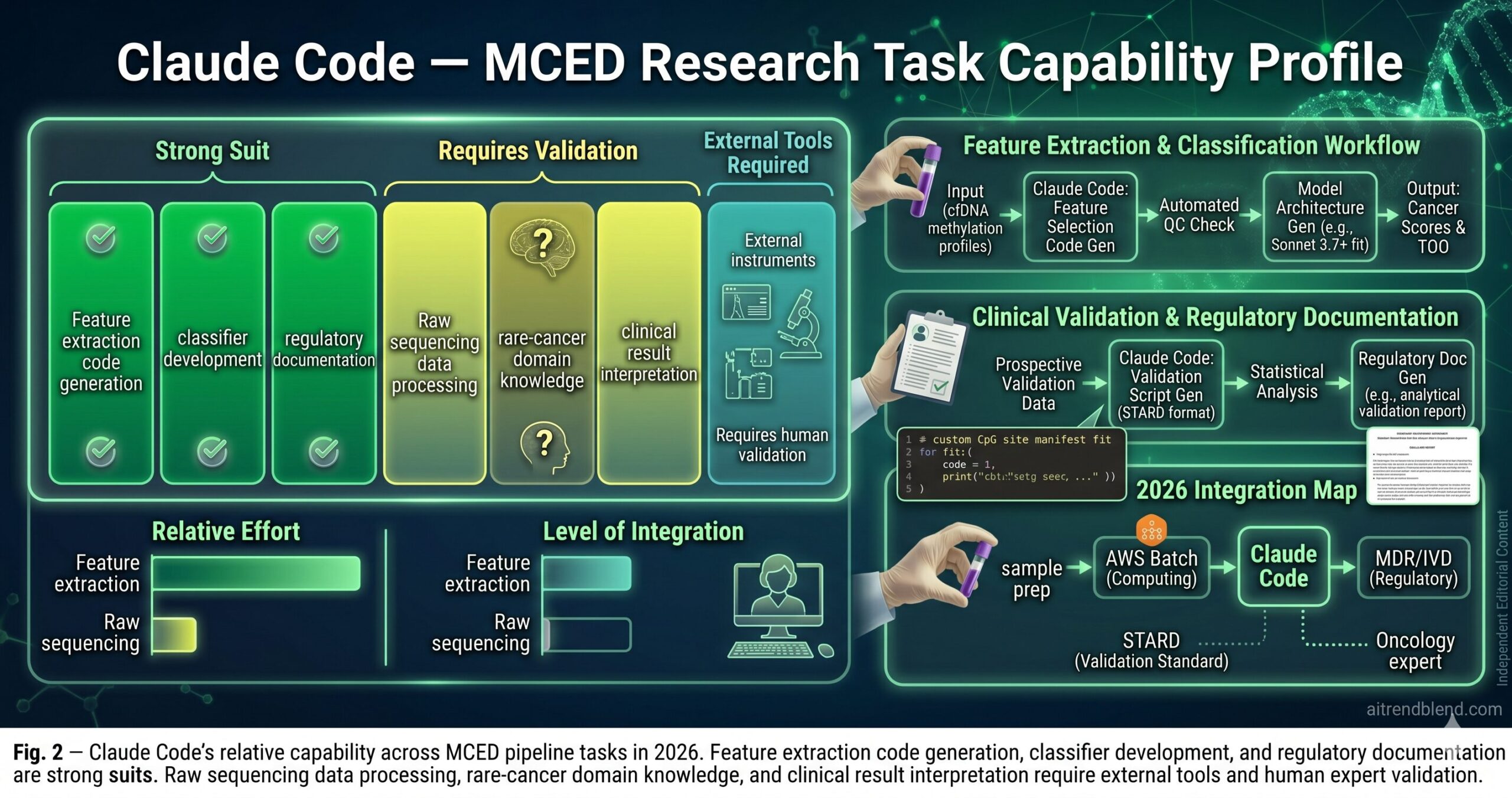
What Claude Code Still Struggles With in MCED Research
Claude Code’s limitations for MCED work are specific, real, and worth understanding before relying on it for high-stakes analyses.
Raw sequencing data processing is beyond its direct reach. Claude Code can generate the bioinformatics scripts — the pysam calls, the bismark parsing, the feature extraction code — but the actual processing of FASTQ and BAM files happens in your compute environment, not in the model. Generating a methylation feature extraction pipeline is fast; running it on a 1,000-sample cohort with 30× WGBS data requires compute infrastructure that Claude Code cannot see or validate. The generated scripts need to be run and profiled in your environment before you trust their outputs. When Claude Code estimates that a script “should run in approximately N hours,” treat that as an order-of-magnitude estimate from a model that has never seen your cluster configuration or storage latency.
Rare cancer type biology has genuine knowledge gaps. For common cancer types — colorectal, lung, breast, prostate — Claude Code’s knowledge of the relevant methylation markers, the typical VAF ranges, and the known confounders is solid. For rare cancer types with limited published literature — ampullary carcinoma, small bowel adenocarcinoma, specific sarcoma subtypes — the generated code may use plausible but not well-validated feature engineering approaches. Any rare-type-specific feature engineering should be reviewed against the primary literature before being used in a study intended for publication or regulatory submission.
Clinical interpretation of borderline results requires human judgment. A cancer score of 0.42 at an operating threshold of 0.40 is a positive result from the classifier’s perspective. Whether that result should trigger a follow-up CT, a colonoscopy, or watchful waiting in a 58-year-old with two comorbidities — that is a clinical decision that requires the treating physician’s judgment and is entirely outside what Claude Code can or should determine. The pipeline generates scores and performance statistics. Clinical decisions based on those scores are the domain of qualified clinicians working within established protocols.
“Finding cancer in a blood draw is an engineering problem and a biological problem and a statistical problem — and solving any one of them without the others produces a test that works in the lab and fails in the clinic.”
— aitrendblend.com Editorial Team, 2026
What This Field Needs — and What It’s Beginning to Have
The capability this guide has mapped is not “how to use AI to analyse blood samples.” It is a structured approach to a computational problem of genuine clinical consequence — one where the gap between a technically impressive classifier and a clinically useful diagnostic tool is defined almost entirely by the rigour of the engineering practices surrounding it. Stage-stratified reporting, data leakage prevention, population-level PPV calculation, pre-specified analytical validation, STARD-compliant reporting — none of these are optional formalities. They are the technical decisions that determine whether a liquid biopsy study produces a result that clinicians can trust to guide patient care or a result that looked good at submission and fails to replicate.
What is changing in 2026 is not the biology of cfDNA — the methylation patterns, the fragment size signals, the end-motif features have been characterised extensively over the past decade. What is changing is the speed and quality of the computational infrastructure that researchers can build around them. Claude Code accelerates the pipeline construction and documentation work that previously consumed a disproportionate fraction of research team capacity. When the engineering scaffolding goes up faster, more time remains for the scientific decisions — the study design choices, the biological interpretation, the clinical partnership work — that actually move the field forward.
There is a category of judgment that this guide’s prompts cannot substitute. Deciding whether a newly identified methylation marker is genuinely cancer-specific or reflects a confounder requires biological knowledge. Determining whether a study’s cohort composition introduces selection bias requires epidemiological expertise. Choosing which cancers to prioritise for a screening programme given cost, follow-up burden, and lead-time bias considerations requires health economics and clinical input. Claude Code builds the pipeline. The scientists, clinicians, and biostatisticians who use it make the decisions that give the pipeline clinical meaning.
The trajectory for AI in MCED points toward three developments over the next 18 to 24 months: transformer-based architectures that process methylation and fragmentation signals jointly rather than as separate modalities, federated learning approaches that allow multi-institution model training without sharing patient-level data, and regulatory frameworks that specifically address AI-based IVD classification under updated FDA guidance. The prompts in this guide will remain relevant as these developments land — the fundamental computational stages of MCED research do not change when the model architectures improve. What will change is how much more is possible with the same data. The researchers positioned to use that capacity well will be the ones who already have the rigorous pipeline practices in place to trust the results it produces.
Try These Prompts Right Now
Open a terminal in your MCED project directory, run claude, and start with Prompt 1 pointed at your BAM files. The fragment profiler will return GC-corrected SFR values and end-motif divergence scores in a single session — the quality characterisation that should precede every downstream classification analysis.
Medical Disclaimer: This article is for informational and educational purposes only. Content does not constitute medical advice, clinical guidance, or regulatory counsel. Consult qualified clinicians, biostatisticians, and regulatory specialists for decisions affecting patient care or IVD development pathways.
Editorial Disclaimer: aitrendblend.com is an independent publication. Not affiliated with Anthropic, GRAIL, Exact Sciences, or any diagnostic company. No sponsored content influenced this article.