
Key points
- PraNet V2 introduces Dual Supervised Reverse Attention, a module that gives a segmentation decoder a separate, independently trained pathway for representing background tissue instead of inferring it as a mathematical complement of the foreground.
- The original PraNet reverse attention mechanism was rule based, entangled foreground and background in shared feature space, and could only handle one class at a time, which made it structurally unusable for multi organ segmentation.
- Plugging the module into three existing state of the art architectures, MIST, Cascaded MERIT, and EMCAD-B2, produced consistent gains on the Synapse multi organ CT benchmark and the ACDC cardiac MRI benchmark with minimal structural changes.
- The biggest single improvement in the paper appears on the ETIS polyp dataset, which was held out entirely from training, and on KiTS19 kidney tumor segmentation, both scenarios where background context is unusually ambiguous.
- An ablation study confirms that the background supervision signal is not decorative. Removing it measurably weakens performance even though it only supervises an auxiliary output.
The awkward relative in every segmentation model
Most medical segmentation systems are trained to find one thing. A polyp. An organ. A lesion. Nobody explicitly teaches the network what the tissue around that target actually looks like. The model learns foreground boundaries entirely from positive examples, so boundary quality tracks how strong the foreground signal is. When contrast is low, which happens constantly in colonoscopy footage where a flat polyp blends smoothly into the surrounding mucosa, there simply is not enough foreground evidence to anchor a confident prediction, and errors pile up right at the edge where clinical decisions matter most.
PraNet, published at MICCAI in 2020 by a team that included several of this paper’s authors, addressed that gap with an idea called reverse attention. The logic was straightforward. Once the model has produced a rough foreground guess, you can flip that guess mathematically to get an implied background map, then feed that implied background back into later refinement stages to sharpen the boundary. It worked well and became a widely copied design pattern across the field.
But that original reverse attention carried three structural problems that only became obvious once researchers tried pushing it toward harder tasks. First, the inversion was purely arithmetic. Each pixel’s background weight was computed as one minus its foreground probability, which means the background signal inherits every mistake the foreground prediction already made and contributes no independent information of its own. Second, foreground and background got fused together inside compressed feature space, tangling the two representations without a clean semantic boundary between them. Third, and most limiting, the single channel design simply had no way to represent more than one foreground class at once, which ruled it out for multi organ or multi class segmentation entirely.
Dual Supervised Reverse Attention, or teaching a network to see what it is not looking for
The paper’s central contribution is a module the authors call Dual Supervised Reverse Attention, abbreviated DSRA. The name signals the key departure from the original design. Instead of computing a background map through a fixed formula, DSRA learns it, with its own parameters and its own supervision signal, entirely separate from the foreground pathway.
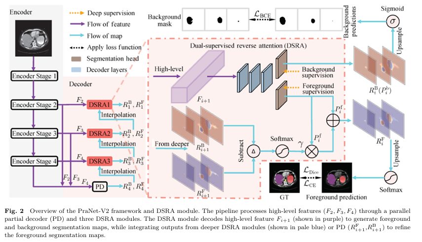
The overall architecture keeps a familiar U-Net shape. An encoder produces four multi scale feature maps at progressively coarser resolutions. The decoder pulls in the three highest level features through a parallel partial decoder, then passes the result through three cascaded DSRA stages that refine the prediction from coarse to fine.
What each DSRA stage actually computes
At decoder stage i, the module takes a high level encoder feature and produces two separate outputs, a foreground map and a background map, each generated by its own segmentation head rather than derived from the other. The foreground output is computed as follows.
The background output is simpler, taken directly from its own head with no reverse term applied to it.
Here P_i^f and P_i^b are the raw outputs of the foreground and background heads, both computed from the same encoder feature through their own convolutional layers. The multiplication term in the first equation is what the authors call the reverse gain, and it is where the real departure from the original design lives.
The reverse gain, and why it is not just an inverted probability anymore
The reverse gain gamma is computed from the deeper stage’s own predictions rather than from an arithmetic complement of the current stage’s foreground guess.
The operator resizes its first argument to match the spatial size of its second argument through bilinear interpolation. So gamma is a softmax normalized difference between the upsampled foreground and background maps from the deeper stage. When the deeper stage’s background confidence is high relative to its foreground confidence at a given location, gamma grows large there, meaning more reverse signal gets injected into the current foreground prediction exactly where the network already believes it is looking at background. That is learned and context sensitive, which is a genuinely different mechanism than one minus a probability.
The per class extension falls naturally out of this design. Because each DSRA stage handles every class through its own segmentation head, the foreground and background maps carry one channel per class, and gamma operates channel by channel. The network can simultaneously represent confidence that a pixel is not liver and separately that it is not spleen, something the original single channel formulation had no way to express.
Background supervision, the other half of the idea
Two segmentation heads only help if the background head actually learns something real. The authors build a per class background mask straight from the ground truth annotations. For each semantic class, a pixel gets a value of one in that class’s background mask if it does not belong to the class, and zero if it does. That produces a multi channel binary target that gives the background head explicit, per class supervision during training rather than leaving it to infer background implicitly.
The total training objective combines three loss terms.
Dice loss applies to the foreground predictions and counteracts the class imbalance that dominates medical segmentation, where background pixels vastly outnumber the tissue a clinician actually cares about. Cross entropy loss adds pixel wise classification signal for the multi class setting. Binary cross entropy applies exclusively to the background predictions, tying each class’s background head to its corresponding background mask.
The ablation results confirm every term earns its place. Dropping the Dice term hurts most on class imbalanced inputs. Dropping either the background BCE term or the classification term weakens the decoupled dual branch design in complementary ways. On ACDC, the full combination reaches 92.31 percent mean Dice. Removing any single term brings that number down, with the smallest drop coming from removing background BCE alone, since it only supervises an auxiliary output rather than the primary prediction.
Binary polyp segmentation results
The authors validate PraNet V2 against the original PraNet on four polyp datasets, CVC-ClinicDB, CVC-300, Kvasir, and the notoriously difficult ETIS set, using two backbones, Res2Net50 and PVTv2-B2, so architectural effects and the module’s own contribution can be told apart.
| Dataset | Backbone | Version | Mean Dice | Mean IoU |
|---|---|---|---|---|
| CVC-300 | Res2Net50 | PraNet-V1 | 87.06 | 79.61 |
| CVC-300 | Res2Net50 | PraNet-V2 | 89.83 | 82.66 |
| CVC-ClinicDB | Res2Net50 | PraNet-V1 | 89.84 | 84.83 |
| CVC-ClinicDB | Res2Net50 | PraNet-V2 | 92.28 | 87.22 |
| ETIS | PVTv2-B2 | PraNet-V1 | 68.32 | 60.02 |
| ETIS | PVTv2-B2 | PraNet-V2 | 76.35 | 68.72 |
Selected rows from the paper’s full results table.
The ETIS result deserves particular attention because those images were never part of training. ETIS was held out entirely as a generalization test. With the PVTv2-B2 backbone, PraNet V2 gains 8.03 points of mean Dice and 8.70 points of mean IoU over the original model on data the network had never seen. A structure similarity measure the paper also reports improves by roughly five points on the same test, indicating the gain is about overall shape and boundary consistency rather than just per pixel accuracy. The fact that the largest improvement in the entire polyp comparison shows up on the one dataset built purely to test generalization is a meaningful pattern, not a coincidence buried in a big table.
Plugging DSRA into three existing state of the art models
The stronger test of the module’s value comes from the multi class experiments. The authors insert DSRA into three separate recent architectures, MIST, Cascaded MERIT, and EMCAD-B2, and evaluate on Synapse, an eight class abdominal CT dataset, and ACDC, a three class cardiac MRI dataset. None of these are toy baselines. All three were already competitive with the field before DSRA was added, so any measurable lift is a real signal rather than an easy win.
Synapse multi organ CT
| Architecture | Mean Dice | HD95 (mm) | Gallbladder Dice |
|---|---|---|---|
| MIST | 81.91 | 14.93 | 71.43 |
| MIST with DSRA | 83.27 | 14.11 | 75.36 |
| EMCAD-B2 | 82.71 | 21.74 | 69.56 |
| EMCAD-B2 with DSRA | 83.75 | 17.77 | 72.79 |
HD95 measures boundary distance in millimeters, lower is better. Gallbladder was chosen because it is typically one of the hardest classes in this dataset.
The gallbladder numbers are worth sitting with. It is small, its border with surrounding liver and fat tissue has low contrast, and its shape varies a lot from one patient scan to the next, which makes it exactly the kind of structure where explicit background modeling should help most. MIST’s gallbladder Dice climbs from 71.43 to 75.36 once DSRA is added, a 3.93 point gain on the class the base model was struggling with hardest. EMCAD-B2’s boundary distance metric drops by close to four millimeters, a change that maps to a visibly tighter, more clinically legible boundary rather than a marginal statistical improvement.
ACDC cardiac MRI
| Architecture | Mean Dice | Right Ventricle | Left Ventricle |
|---|---|---|---|
| MIST | 91.73 | 89.98 | 95.84 |
| MIST with DSRA | 92.31 | 90.82 | 96.04 |
| Cascaded MERIT | 91.78 | 90.36 | 95.79 |
| Cascaded MERIT with DSRA | 92.28 | 91.27 | 96.19 |
The right ventricle consistently receives the largest single class improvement in this table. It has a thin, irregular wall that is genuinely difficult to trace precisely, which again lines up with the pattern that DSRA helps most exactly where boundary ambiguity is worst.
Where PraNet V2 sits against SAM based alternatives
Medical segmentation research in the current cycle leans heavily on large foundation models, SAM variants with prompt engineering, and diffusion based approaches. PraNet V2 is deliberately a narrower contribution than any of that. It targets one specific architectural gap and closes it with minimal structural overhead rather than chasing a bigger, more general model.
The comparison against SAM based systems is genuinely informative. PraNet V2 outperforms BiomedParse across every reported metric without requiring any input prompt at all, which matters because BiomedParse and similar systems typically need a point or box prompt to work well. Against MedSAM, PraNet V2 loses when MedSAM is given a tight, accurate bounding box with only a two percent margin of error, which makes sense since that prompt is essentially handing the model the answer. But PraNet V2 wins across every metric once that bounding box prompt becomes even slightly imprecise, at an eight percent margin. For a fully automatic method going up against one that receives partial geometric information about the correct answer, that is a strong showing.
The paper’s most dramatic single result appears in an appendix rather than the main text. On KiTS19, a kidney tumor segmentation benchmark, EMCAD-B2 with DSRA gains 10.61 points of mean Dice over the same base model without DSRA. Kidney tumors tend to have unusually ambiguous boundaries against surrounding normal tissue that looks structurally similar, which is precisely the scenario where an explicit, independently learned background representation should offer the most benefit, and the result is consistent with that reasoning.
Clinical translation gap
Every number reported above comes from standard public benchmark splits, Synapse, ACDC, the polyp datasets, and KiTS19 in the appendix. That is the normal way computer vision research validates a method, and it is a meaningfully different thing from prospective validation in an actual clinical workflow. The paper as summarized here does not report testing across multiple hospitals, multiple scanner manufacturers, or multiple annotation teams, which are the conditions where segmentation models most often lose accuracy compared to their published benchmark numbers. ETIS is the one dataset explicitly used as a genuine holdout test for generalization, and that is exactly why its result is the headline gain in the polyp comparison. Synapse, ACDC, and KiTS19 are evaluated on splits drawn from the same underlying data distribution as their training sets, which is standard practice but is not the same claim as generalization to a new hospital’s imaging pipeline. None of this means the method does not work. It means the distance between a strong benchmark result and a tool a clinician could rely on during a real procedure has not been measured yet in what this paper reports, and that gap is where the real work of clinical translation still has to happen.
Honest limitations
The source material for this analysis does not report patient level sample sizes, demographic composition, or inter rater annotation agreement for the datasets used, which makes it hard to independently judge how representative these benchmarks are of the patient populations a deployed tool would eventually see. Synapse and ACDC are widely used, well curated academic benchmarks, but curation itself can introduce selection effects, since cases that are ambiguous or poorly imaged are sometimes excluded during dataset construction in ways that are not always fully documented.
Generalization evidence is also uneven across tasks. The ETIS result is a genuine out of distribution test and it is the strongest evidence in the paper that DSRA’s benefit is not just memorization. The Synapse, ACDC, and KiTS19 results, while consistent and encouraging, come from standard splits rather than held out external cohorts, so they speak more to architectural improvement than to real world robustness. The frozen, non fine tuned segmentation backbone design that made DSRA easy to plug into three different architectures is also, by construction, only as good as those base architectures already were. DSRA improves what a given decoder does with the features it receives. It does not fix a fundamentally weak encoder or compensate for genuinely low quality input imaging.
Finally, this is a peer reviewed methods paper in a computer vision venue, Computational Visual Media, rather than a clinical trial published in a medical journal with regulatory oversight. That distinction matters. A strong Dice score improvement is evidence a model localizes anatomy more precisely under laboratory conditions. It is not evidence of clinical utility, workflow integration, or patient outcomes, and nothing in this analysis should be read as a claim that it is.
Complete reference implementation in PyTorch
The implementation below is a full, runnable translation of PraNet V2 as described above, including the DSRA module, the parallel partial decoder, background mask construction, the combined Dice, cross entropy, and binary cross entropy loss, a lightweight encoder standing in for Res2Net50 or PVTv2-B2, and a smoke test that exercises the full forward pass, loss computation, and a short training loop against dummy data. It is an educational reimplementation, not the authors’ original codebase.
# PraNet-V2 reference implementation
# Dual Supervised Reverse Attention for medical image segmentation
# Educational reimplementation, not the original authors' code

import math
import torch
import torch.nn as nn
import torch.nn.functional as F
from torch import Tensor
from torch.utils.data import DataLoader, Dataset
from typing import List, Optional, Tuple, Dict


# ---- Configuration ----

class PraNetV2Config:
    def __init__(self, **kwargs):
        self.num_classes = 1
        self.img_size = 352
        self.in_channels = 3
        self.encoder_channels = [64, 256, 512, 1024]
        self.decoder_channels = 64
        self.loss_weights = (1.0, 1.0, 0.5)
        for k, v in kwargs.items():
            setattr(self, k, v)


# ---- Encoder backbone ----

class ConvBnRelu(nn.Module):
    def __init__(self, in_c, out_c, k=3, s=1, p=1):
        super().__init__()
        self.block = nn.Sequential(
            nn.Conv2d(in_c, out_c, k, stride=s, padding=p, bias=False),
            nn.BatchNorm2d(out_c),
            nn.ReLU(inplace=True),
        )

    def forward(self, x):
        return self.block(x)


class SimpleEncoder(nn.Module):
    # Stands in for Res2Net50 or PVTv2-B2 for smoke testing
    def __init__(self, in_channels=3):
        super().__init__()
        self.stage1 = nn.Sequential(ConvBnRelu(in_channels, 64, k=7, s=2, p=3), ConvBnRelu(64, 64))
        self.stage2 = nn.Sequential(nn.MaxPool2d(2), ConvBnRelu(64, 256), ConvBnRelu(256, 256))
        self.stage3 = nn.Sequential(nn.MaxPool2d(2), ConvBnRelu(256, 512), ConvBnRelu(512, 512))
        self.stage4 = nn.Sequential(nn.MaxPool2d(2), ConvBnRelu(512, 1024), ConvBnRelu(1024, 1024))

    def forward(self, x):
        f1 = self.stage1(x)
        f2 = self.stage2(f1)
        f3 = self.stage3(f2)
        f4 = self.stage4(f3)
        return f1, f2, f3, f4


# ---- Parallel partial decoder ----

class ChannelReducer(nn.Module):
    def __init__(self, in_c, out_c):
        super().__init__()
        self.conv = ConvBnRelu(in_c, out_c, k=1, s=1, p=0)

    def forward(self, x):
        return self.conv(x)


class ParallelPartialDecoder(nn.Module):
    def __init__(self, enc_channels, mid_channels=64, num_classes=1):
        super().__init__()
        c2, c3, c4 = enc_channels
        self.reduce2 = ChannelReducer(c2, mid_channels)
        self.reduce3 = ChannelReducer(c3, mid_channels)
        self.reduce4 = ChannelReducer(c4, mid_channels)
        self.fuse = nn.Sequential(ConvBnRelu(mid_channels * 3, mid_channels), ConvBnRelu(mid_channels, mid_channels))
        self.fg_head = nn.Conv2d(mid_channels, num_classes, kernel_size=1)
        self.bg_head = nn.Conv2d(mid_channels, num_classes, kernel_size=1)

    def forward(self, f2, f3, f4):
        h, w = f2.shape[2], f2.shape[3]
        r2, r3, r4 = self.reduce2(f2), self.reduce3(f3), self.reduce4(f4)
        r3 = F.interpolate(r3, size=(h, w), mode="bilinear", align_corners=True)
        r4 = F.interpolate(r4, size=(h, w), mode="bilinear", align_corners=True)
        feat = self.fuse(torch.cat([r2, r3, r4], dim=1))
        return feat, self.fg_head(feat), self.bg_head(feat)


# ---- DSRA module, the paper's core contribution ----

class DSRAModule(nn.Module):
    def __init__(self, in_channels, mid_channels=64, num_classes=1):
        super().__init__()
        self.num_classes = num_classes
        self.decoder_layers = nn.Sequential(
            ChannelReducer(in_channels, mid_channels),
            ConvBnRelu(mid_channels, mid_channels),
            ConvBnRelu(mid_channels, mid_channels),
        )
        self.fg_head = nn.Conv2d(mid_channels, num_classes, kernel_size=1)
        self.bg_head = nn.Conv2d(mid_channels, num_classes, kernel_size=1)

    def forward(self, f_enc, r_fg_deep, r_bg_deep):
        b, c_in, h, w = f_enc.shape
        feat = self.decoder_layers(f_enc)
        p_fg = self.fg_head(feat)
        p_bg = self.bg_head(feat)

        r_fg_up = F.interpolate(r_fg_deep, size=(h, w), mode="bilinear", align_corners=True)
        r_bg_up = F.interpolate(r_bg_deep, size=(h, w), mode="bilinear", align_corners=True)
        diff = r_fg_up - r_bg_up

        if self.num_classes > 1:
            gamma = F.softmax(diff, dim=1)
        else:
            gamma = torch.sigmoid(diff)

        r_fg = p_fg + p_fg * gamma   # Equation 1
        r_bg = p_bg                   # Equation 2
        return r_fg, r_bg


# ---- Full PraNet-V2 model ----

class PraNetV2(nn.Module):
    def __init__(self, config=None, encoder=None):
        super().__init__()
        cfg = config or PraNetV2Config()
        self.cfg = cfg
        c = cfg.decoder_channels
        enc_ch = cfg.encoder_channels

        self.encoder = encoder if encoder is not None else SimpleEncoder(cfg.in_channels)
        self.pd = ParallelPartialDecoder(enc_ch[1:], mid_channels=c, num_classes=cfg.num_classes)
        self.dsra3 = DSRAModule(enc_ch[3], mid_channels=c, num_classes=cfg.num_classes)
        self.dsra2 = DSRAModule(enc_ch[2], mid_channels=c, num_classes=cfg.num_classes)
        self.dsra1 = DSRAModule(enc_ch[1], mid_channels=c, num_classes=cfg.num_classes)

    def forward(self, x):
        b, _, h_in, w_in = x.shape
        f1, f2, f3, f4 = self.encoder(x)
        _, r4_fg, r4_bg = self.pd(f2, f3, f4)
        r3_fg, r3_bg = self.dsra3(f4, r4_fg, r4_bg)
        r2_fg, r2_bg = self.dsra2(f3, r3_fg, r3_bg)
        r1_fg, r1_bg = self.dsra1(f2, r2_fg, r2_bg)

        def up(t):
            return F.interpolate(t, size=(h_in, w_in), mode="bilinear", align_corners=True)

        return {
            "r1_fg": up(r1_fg), "r1_bg": up(r1_bg),
            "r2_fg": up(r2_fg), "r2_bg": up(r2_bg),
            "r3_fg": up(r3_fg), "r3_bg": up(r3_bg),
            "r4_fg": up(r4_fg), "r4_bg": up(r4_bg),
        }


# ---- Background mask construction ----

def build_background_mask(seg_mask, num_classes):
    one_hot = F.one_hot(seg_mask.long(), num_classes).permute(0, 3, 1, 2).float()
    return 1.0 - one_hot


def build_binary_background_mask(binary_mask):
    if binary_mask.dim() == 3:
        binary_mask = binary_mask.unsqueeze(1)
    return 1.0 - binary_mask


# ---- Losses, Equation 4 ----

class BinaryDiceLoss(nn.Module):
    def __init__(self, smooth=1e-5):
        super().__init__()
        self.smooth = smooth

    def forward(self, pred, target):
        p = torch.sigmoid(pred)
        if target.dim() == 3:
            target = target.unsqueeze(1)
        target = target.float()
        p_flat, g_flat = p.reshape(p.shape[0], -1), target.reshape(target.shape[0], -1)
        inter = (p_flat * g_flat).sum(dim=-1)
        denom = p_flat.sum(dim=-1) + g_flat.sum(dim=-1)
        dice = (2 * inter + self.smooth) / (denom + self.smooth)
        return 1.0 - dice.mean()


class MultiClassDiceLoss(nn.Module):
    def __init__(self, num_classes, smooth=1e-5):
        super().__init__()
        self.num_classes, self.smooth = num_classes, smooth

    def forward(self, pred, target):
        p = F.softmax(pred, dim=1)
        one_hot = F.one_hot(target.long(), self.num_classes).permute(0, 3, 1, 2).float()
        p_flat = p.reshape(p.shape[0], self.num_classes, -1)
        g_flat = one_hot.reshape(one_hot.shape[0], self.num_classes, -1)
        omega = 1.0 / self.num_classes
        inter = (p_flat * g_flat).sum(dim=-1)
        denom = p_flat.pow(2).sum(dim=-1) + g_flat.pow(2).sum(dim=-1)
        dice_pc = (2 * omega * inter) / (denom + self.smooth)
        return 1.0 - dice_pc.mean()


class PraNetV2Loss(nn.Module):
    def __init__(self, num_classes=1, weights=(1.0, 1.0, 0.5), stage_weights=(1.0, 0.8, 0.6, 0.4)):
        super().__init__()
        self.num_classes = num_classes
        self.w1, self.w2, self.w3 = weights
        self.stage_weights = stage_weights
        self.binary = num_classes == 1
        self.dice_loss = BinaryDiceLoss() if self.binary else MultiClassDiceLoss(num_classes)
        if not self.binary:
            self.ce_loss = nn.CrossEntropyLoss()
        self.bce_loss = nn.BCEWithLogitsLoss()

    def _stage_loss(self, r_fg, r_bg, fg_gt, bg_mask):
        if self.binary:
            l_dice = self.dice_loss(r_fg, fg_gt)
            target = fg_gt.unsqueeze(1).float() if fg_gt.dim() == 3 else fg_gt
            l_ce = F.binary_cross_entropy_with_logits(r_fg, target)
        else:
            l_dice = self.dice_loss(r_fg, fg_gt)
            l_ce = self.ce_loss(r_fg, fg_gt.long())
        l_bce = self.bce_loss(r_bg, bg_mask)
        return self.w1 * l_dice + self.w2 * l_ce + self.w3 * l_bce

    def forward(self, preds, fg_gt, bg_mask):
        stage_keys = [("r1_fg", "r1_bg"), ("r2_fg", "r2_bg"), ("r3_fg", "r3_bg"), ("r4_fg", "r4_bg")]
        total = torch.tensor(0.0, device=fg_gt.device)
        for sw, (fk, bk) in zip(self.stage_weights, stage_keys):
            total = total + sw * self._stage_loss(preds[fk], preds[bk], fg_gt, bg_mask)
        return total


# ---- Metrics ----

def compute_dice_binary(pred_logits, target, eps=1e-5):
    pred_bin = (torch.sigmoid(pred_logits) > 0.5).float()
    if target.dim() == 3:
        target = target.unsqueeze(1)
    target = target.float()
    b = pred_bin.shape[0]
    p, g = pred_bin.reshape(b, -1), target.reshape(b, -1)
    inter = (p * g).sum(dim=-1)
    denom = p.sum(dim=-1) + g.sum(dim=-1)
    return ((2 * inter + eps) / (denom + eps)).mean().item()


class SegMetrics:
    def __init__(self, num_classes=1):
        self.num_classes = num_classes
        self.reset()

    def reset(self):
        self.dice_sum, self.count = 0.0, 0

    @torch.no_grad()
    def update(self, pred_logits, target):
        if self.num_classes == 1:
            self.dice_sum += compute_dice_binary(pred_logits, target)
        else:
            pred_cls = pred_logits.argmax(dim=1)
            eps, dice_vals = 1e-5, []
            for c in range(self.num_classes):
                p, g = (pred_cls == c).float(), (target == c).float()
                tp = (p * g).sum()
                fp = (p * (1 - g)).sum()
                fn = ((1 - p) * g).sum()
                dice_vals.append((2 * tp + eps) / (2 * tp + fp + fn + eps))
            self.dice_sum += torch.stack(dice_vals).mean().item()
        self.count += 1

    def result(self):
        return {"mDice": self.dice_sum / max(1, self.count)}


# ---- Dummy datasets for smoke testing ----

class PolypDummyDataset(Dataset):
    def __init__(self, num_samples=16, img_size=352):
        self.n, self.sz = num_samples, img_size

    def __len__(self):
        return self.n

    def __getitem__(self, idx):
        img = torch.randn(3, self.sz, self.sz)
        mask = torch.randint(0, 2, (self.sz, self.sz)).float()
        return img, mask


class SynapseDummyDataset(Dataset):
    def __init__(self, num_samples=16, img_size=352, num_classes=9):
        self.n, self.sz, self.nc = num_samples, img_size, num_classes

    def __len__(self):
        return self.n

    def __getitem__(self, idx):
        img = torch.randn(1, self.sz, self.sz)
        mask = torch.randint(0, self.nc, (self.sz, self.sz))
        return img, mask


# ---- Training loop ----

def train_one_epoch(model, loader, optimizer, criterion, device, num_classes):
    model.train()
    total_loss = 0.0
    for imgs, masks in loader:
        imgs, masks = imgs.to(device), masks.to(device)
        bg_mask = build_binary_background_mask(masks.float()) if num_classes == 1 else build_background_mask(masks, num_classes)
        optimizer.zero_grad()
        preds = model(imgs)
        loss = criterion(preds, masks, bg_mask)
        loss.backward()
        torch.nn.utils.clip_grad_norm_(model.parameters(), max_norm=1.0)
        optimizer.step()
        total_loss += loss.item()
    return total_loss / len(loader)


@torch.no_grad()
def validate(model, loader, criterion, metrics, device, num_classes):
    model.eval()
    metrics.reset()
    total_loss = 0.0
    for imgs, masks in loader:
        imgs, masks = imgs.to(device), masks.to(device)
        bg_mask = build_binary_background_mask(masks.float()) if num_classes == 1 else build_background_mask(masks, num_classes)
        preds = model(imgs)
        total_loss += criterion(preds, masks, bg_mask).item()
        metrics.update(preds["r1_fg"], masks)
    return total_loss / len(loader), metrics.result()


# ---- Smoke test ----

if __name__ == "__main__":
    torch.manual_seed(42)
    device = torch.device("cpu")

    print("Binary polyp forward pass")
    cfg1 = PraNetV2Config(num_classes=1, in_channels=3)
    model1 = PraNetV2(cfg1).to(device)
    x1 = torch.randn(2, 3, 352, 352)
    with torch.no_grad():
        out1 = model1(x1)
    assert out1["r1_fg"].shape == (2, 1, 352, 352)
    print("  r1_fg shape", tuple(out1["r1_fg"].shape))

    print("Multi class Synapse style forward pass")
    cfg2 = PraNetV2Config(num_classes=9, in_channels=1)
    model2 = PraNetV2(cfg2).to(device)
    x2 = torch.randn(2, 1, 352, 352)
    with torch.no_grad():
        out2 = model2(x2)
    assert out2["r1_fg"].shape == (2, 9, 352, 352)
    print("  r1_fg shape", tuple(out2["r1_fg"].shape))

    print("Background mask construction")
    seg_gt = torch.randint(0, 9, (2, 352, 352))
    bg_mask = build_background_mask(seg_gt, num_classes=9)
    assert bg_mask.shape == (2, 9, 352, 352)
    print("  bg_mask shape", tuple(bg_mask.shape))

    print("Loss computation")
    crit_bin = PraNetV2Loss(num_classes=1)
    fg_gt_bin = torch.randint(0, 2, (2, 352, 352)).float()
    loss_bin = crit_bin(out1, fg_gt_bin, build_binary_background_mask(fg_gt_bin))
    print("  binary loss", loss_bin.item())

    crit_mc = PraNetV2Loss(num_classes=9)
    loss_mc = crit_mc(out2, seg_gt, bg_mask)
    print("  multi class loss", loss_mc.item())

    print("Short training run on dummy polyp data")
    train_ds = PolypDummyDataset(num_samples=8)
    val_ds = PolypDummyDataset(num_samples=4)
    train_loader = DataLoader(train_ds, batch_size=2, shuffle=True)
    val_loader = DataLoader(val_ds, batch_size=2, shuffle=False)
    optimizer = torch.optim.Adam(model1.parameters(), lr=1e-4)
    metrics = SegMetrics(num_classes=1)
    for epoch in range(2):
        tr_loss = train_one_epoch(model1, train_loader, optimizer, crit_bin, device, num_classes=1)
        val_loss, res = validate(model1, val_loader, crit_bin, metrics, device, num_classes=1)
        print(f"  epoch {epoch} train {tr_loss:.4f} val {val_loss:.4f} mDice {res['mDice']:.4f}")

    print("All checks passed.")
Conclusion
PraNet V2’s real achievement is narrower and more useful than it might sound at first. Rather than proposing another large, general purpose architecture, the authors identified one specific gap in a mechanism they themselves had built five years earlier, worked out precisely why it broke down under multi class and low contrast conditions, and closed that gap with a module that drops into three unrelated existing architectures with minimal structural disruption. The consistency of the gain across MIST, Cascaded MERIT, and EMCAD-B2, on datasets as different as abdominal CT and cardiac MRI, is the strongest evidence that the fix targets something genuinely missing in the underlying decoder design rather than something specific to any one model.
The conceptual shift worth carrying forward is that background is not nothing. A model that only ever learns what a target looks like, and infers everything else as an arithmetic leftover, is discarding a real source of boundary information. Giving the background its own supervised pathway, with its own loss and its own learned parameters, let the network discover texture and context cues about surrounding tissue that a purely foreground driven design has no way to access. That idea plausibly generalizes past medical imaging to any dense prediction task where the thing you are not looking for still carries information about the thing you are.
The honest caveats matter as much as the gains. Every number in this analysis comes from public benchmark splits rather than prospective clinical validation, sample size and demographic detail were not reported in the material available here, and only one dataset, ETIS, was used as a genuine test of generalization to unseen data. The gallbladder and right ventricle results are compelling because they land exactly where boundary ambiguity is worst, which is a good sign the mechanism is doing what it claims. It is not the same as evidence that the tool is ready for a hospital workflow.
Future work the authors gesture toward includes extending the comparison against a wider range of foundation model baselines and testing the module on more anatomical regions. A natural next step beyond what is reported here would be evaluating DSRA under genuine multi site conditions, different scanners, different populations, different annotation protocols, since that is precisely the setting where the gap between benchmark performance and real usefulness tends to show up.
Taken as a whole, PraNet V2 is a good example of research that improves a widely used idea by figuring out exactly where it was quietly broken rather than by making it bigger. The module is simple enough to describe in four equations and small enough to add to an existing pipeline in an afternoon, and the ablation study backs up that the improvement is coming from the mechanism it claims rather than from extra parameters alone.
Frequently asked questions
What is Dual Supervised Reverse Attention and how does it differ from the original PraNet design
Dual Supervised Reverse Attention, or DSRA, gives a segmentation decoder a separate background prediction head with its own loss, instead of computing background as one minus the foreground probability the way the original PraNet did. That independent supervision lets the network learn genuine background texture cues rather than inheriting whatever errors the foreground prediction already made.
Does adding DSRA require redesigning an existing segmentation architecture
No. The paper demonstrates DSRA added to three separate, already competitive architectures, MIST, Cascaded MERIT, and EMCAD-B2, with consistent gains across all three. The module needs two segmentation heads per decoder stage and a background mask built from existing ground truth labels, which is a modest structural addition rather than a rebuild.
How much does DSRA actually improve segmentation accuracy
Gains vary by dataset and structure. On the ETIS polyp dataset, which was held out entirely from training, mean Dice improved by 8.03 points. On Synapse, the hardest class, gallbladder, improved by 3.93 points of Dice. On the appendix KiTS19 kidney tumor benchmark, EMCAD-B2 with DSRA gained 10.61 points of mean Dice over the same model without it.
Is PraNet V2 only useful for polyp segmentation
No. Beyond the original polyp focus, the paper evaluates DSRA on Synapse, an eight class abdominal CT dataset, ACDC, a three class cardiac MRI dataset, and KiTS19, a kidney tumor dataset, with gains reported on every one.
How does PraNet V2 compare to SAM based segmentation models
PraNet V2 outperforms BiomedParse on every reported metric without needing any input prompt. Against MedSAM, it loses only when MedSAM receives a tight, highly accurate bounding box prompt, and wins across every metric once that prompt becomes even slightly imprecise, which is a strong result for a fully automatic method.
What are the main limitations of this research for real clinical use
All reported results come from public benchmark datasets evaluated with standard splits, not prospective validation across multiple hospitals or scanners. Only the ETIS polyp dataset served as a genuine held out generalization test. Sample size and demographic detail for the datasets were not reported in the material this analysis is based on, and the method has not been validated as a clinical decision support tool.
Go deeper
Read the full paper for complete per organ results, qualitative comparisons, and the SAM based model comparisons summarized above.
Read the paper, DOI 10.26599/CVM.2025.9450510 View the code on GitHubThis analysis is based on the published paper and an independent evaluation of its claims.
Related reading
For background on the multi organ CT and cardiac MRI benchmarks referenced above, see the site’s coverage of MT-Net’s 3D retinal microvascular segmentation work and the discussion of uncertainty estimation in breast tumor segmentation, both of which run into the same background modeling and generalization questions raised here. For a look at model architecture design in a very different segmentation setting, the piece on GeoSAM2’s prompt controllable 3D part segmentation is also relevant, and readers interested in the broader medical AI category can browse the full medical AI archive for related coverage.