Teaching Three Different Brains to Agree — How Weak-Mamba-UNet Segments Hearts from Scribbles
Ziyang Wang at Oxford and Chao Ma introduce Weak-Mamba-UNet: the first weakly-supervised framework that runs CNN, Vision Transformer, and Visual Mamba together under scribble supervision, letting each architecture’s strengths cover the others’ blind spots. On MRI cardiac segmentation, it achieves Dice 0.9171 and HD 3.96 — surpassing every single-network baseline by a meaningful margin.
Consider the problem a radiologist faces when asked to annotate a thousand cardiac MRI scans for an AI training project. Pixel-perfect segmentation masks — outlining every voxel of myocardium, left ventricle, and right ventricle — take minutes per slice and hours per patient. Multiply that across a dataset large enough to train a modern deep learning model and you have a problem that is, frankly, not going to get solved on a clinical budget. Scribble annotations are the pragmatic alternative: a radiologist draws a rough line through each structure, marks the background with a few strokes, and moves on. Ziyang Wang and Chao Ma’s Weak-Mamba-UNet is built around the question of what you can actually do with that incomplete signal.
The Core Problem: Scribbles Are Sparse, and That’s the Whole Point
Scribble-based annotation occupies a philosophically interesting middle ground. It is not as cheap as image-level tags (which tell you only whether a structure is present, not where). It is not as expensive as full segmentation masks. And it is not random — a scribble placed through the center of the left ventricle genuinely captures the appearance of left-ventricular tissue, just not its complete shape.
The challenge is that everything a standard segmentation loss function wants to do — compare predicted class probabilities at every pixel against a ground truth label — falls apart when 80% of pixels carry no label at all. You cannot penalize the network for predicting “myocardium” at a pixel that the annotator simply never drew a stroke through, because that pixel might actually be myocardium. Standard cross-entropy on the full image would treat unlabeled pixels as wrong for every class, which is catastrophically incorrect.
The cleanest solution to this is partial cross-entropy: compute the loss only at pixels where a scribble annotation exists, ignore everything else. That gets you a functioning training signal, but a thin one. The network has no incentive to produce coherent predictions in the unlabeled regions — it could predict random noise between the scribble strokes and the partial loss would not care. That is where pseudo labels enter the picture, and where the three-network architecture of Weak-Mamba-UNet becomes the key design idea.
No single architecture is equally good at local texture (CNN), global context (Transformer), and long-range sequential dependencies (Mamba). But if you train all three simultaneously and let each network’s dense predictions serve as soft supervision for the others, you get an iterative refinement loop that fills in the gaps left by sparse scribble annotations — without ever requiring a fully labeled image.
Why Three Architectures? A Brief History of Their Complementary Blind Spots
UNet — still the workhorse of medical image segmentation six years after its introduction — is built on convolutions. Its strength is local: it excels at capturing fine-grained texture patterns and spatial relationships within a small receptive field. Its skip connections preserve spatial detail across the encoder-decoder gap. The weakness is global: standard convolutions cannot, without significant depth, relate features from opposite ends of an image.
The Swin Transformer addresses that gap through shifted-window attention. By partitioning the image into non-overlapping windows and applying self-attention within each window — then shifting the windows each layer to allow cross-window interaction — SwinUNet captures long-range spatial relationships that convolutions miss. The trade-off is that the attention mechanism is computationally heavy and the model needs ImageNet pretraining to reach competitive performance on limited medical datasets.
Visual Mamba, the newest entrant, builds on the State Space Model (SSM) framework developed for sequence modeling. Mamba processes image patches as a long sequence, updating a compact hidden state as it scans through the image. The key property is efficiency: unlike self-attention, Mamba’s computation scales linearly with sequence length rather than quadratically. That makes it particularly attractive for high-resolution medical images where attention would be prohibitively expensive. It also brings a different flavor of long-range dependency — not the global pair-wise comparison of attention, but a recurrent propagation of state across the sequence.
The three architectures encode the same image differently. That diversity is the resource Weak-Mamba-UNet exploits.
The Framework Architecture: Cross-Supervision as a Feedback Loop
Three Networks, One Loss, One Shared Goal
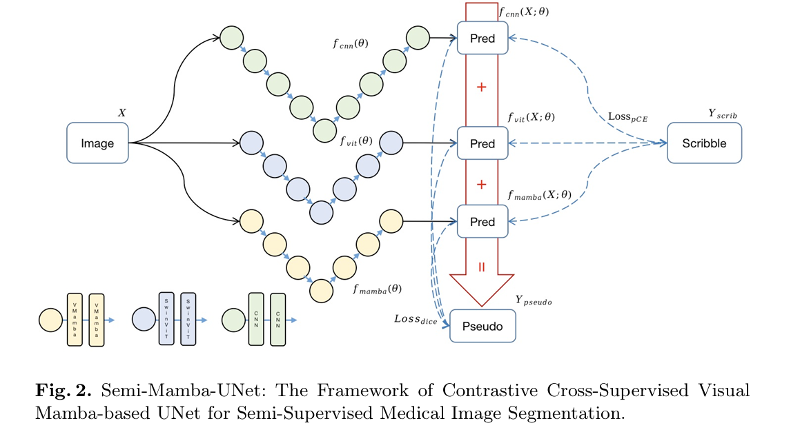
All three networks — UNet (CNN), SwinUNet (ViT), and MambaUNet (VMamba) — receive the same input image X and produce individual predictions. Each prediction is a soft probability map over the four classes: right ventricle, left ventricle, myocardium, and background. The network parameters are initialized independently, which ensures the three models start from genuinely different perspectives rather than converging to the same local minimum early in training.
The total training loss for each network is the sum of two terms. The first is partial cross-entropy against the scribble annotations — computed only at labeled pixels, ignoring everything else. The second is a dice loss against a composite pseudo label. The total objective across all three networks is:
The Random Weighting Trick
Here is a detail that looks minor but matters a great deal in practice. The weighting factors α, β, and γ for the pseudo label ensemble are not fixed — they are randomly sampled at each training iteration, constrained only to sum to 1. This introduces a stochastic perturbation into the pseudo label signal, preventing any single network from dominating the supervision of the others. It is conceptually similar to data augmentation, except applied to the label space rather than the input image. The randomness forces all three networks to remain meaningfully different, because neither can learn to simply copy the output of the strongest network.
Without this randomization, a natural failure mode would be early collapse: the strongest network at any given stage of training would produce pseudo labels that the other two learn to imitate, eventually erasing the architectural diversity that makes the ensemble useful. The random weighting prevents this feedback collapse while still allowing mutual improvement.
WEAK-MAMBA-UNET — FULL FRAMEWORK DIAGRAM
═══════════════════════════════════════════════════════════════════

INPUT: X ∈ R^{H×W}  (224×224 grayscale MRI slice)
        Y_scrib ∈ {0,1,2,3,None}  (RVC, LVC, MYO, BG, unlabeled)

PARALLEL FORWARD PASSES (all three networks see the same X):
  ┌──────────────────────────────────────────────────────┐
  │  f_cnn(X; θ_cnn)     → Y_cnn    [UNet, CNN]         │
  │  f_vit(X; θ_vit)     → Y_vit    [SwinUNet, ViT]     │
  │  f_mamba(X; θ_mamba) → Y_mamba  [MambaUNet, VMamba] │
  └──────────────────────────────────────────────────────┘

PSEUDO LABEL GENERATION (at each iteration):
  Sample α, β, γ ~ Dirichlet or uniform, s.t. α+β+γ = 1
  Y_pseudo = α·Y_cnn + β·Y_vit + γ·Y_mamba   (soft ensemble)
  Ŷ_pseudo = argmax(Y_pseudo)                  (hard label for dice)

LOSS COMPUTATION (per network i ∈ {cnn, vit, mamba}):
  L_pce_i  = − Σ_{j∈Ω_L} Σ_k  y_s[j,k]·log(y_i[j,k])
              (only at scribble-annotated pixels)
  L_dice_i = 1 − Dice(softmax(f_i(X)), Y_pseudo)
  L_i      = L_pce_i + L_dice_i

TOTAL LOSS:
  L_total = L_cnn + L_vit + L_mamba

OPTIMIZATION:
  SGD, lr=0.01, momentum=0.9, weight_decay=1e-4
  Batch size=24, 30,000 iterations
  Validate every 200 iterations, save on val improvement

EVALUATION:
  Predictions from any single network (or ensemble) vs dense GT
  Metrics: Dice, Accuracy, Precision, Sensitivity, Specificity, HD95, ASD
What Makes MambaUNet Different: State Space Models Explained Simply
State Space Models are not a new idea — they have roots in classical control theory and signal processing. The key insight Mamba brings to vision is a selective state space: rather than updating its hidden state identically for every input token, Mamba learns to selectively compress or amplify different inputs based on their content. Irrelevant patches get summarized quickly; important patches get more “space” in the model’s memory.
For medical image segmentation, this selectivity is physically meaningful. In a cardiac MRI slice, most of the image is chest wall, lung, and background tissue — not the cardiac structures you actually care about. A recurrent model that learns to compress the uninteresting background while retaining detailed state about the ventricular boundaries is doing something qualitatively similar to the radiologist who scans quickly over familiar anatomy before examining the region of interest more carefully.
MambaUNet applies this principle in a U-shaped encoder-decoder architecture, replacing the CNN or attention blocks with Visual Mamba blocks at each level. The result is a model that captures long-range dependencies — relationships between distant parts of the cardiac anatomy — without the quadratic memory cost of full attention, and without the receptive field limitations of convolutions.
“The WSL framework consisting of SwinUNet performs less well, which indicates that although the performance of the independent SwinUNet algorithm is able to outperform that of UNet, there is a lack of differentiation between the Multi-SwinUNet models.” — Wang & Ma, Weak-Mamba-UNet (arXiv 2402.10887)
This observation from the ablation study is one of the most instructive findings in the paper. Running three copies of the same architecture — even a strong one like SwinUNet — produces a degenerate framework where the three networks converge to nearly identical solutions. The pseudo label becomes the average of three nearly identical predictions, which provides no useful signal beyond what any single network already knows. Diversity is not optional in this framework; it is the mechanism by which cross-supervision works.
Benchmark Results: Reading the Numbers Carefully
| Method + Network | Dice ↑ | Acc ↑ | Pre ↑ | Sen ↑ | HD95 ↓ | ASD ↓ |
|---|---|---|---|---|---|---|
| pCE + UNet | 0.7620 | 0.9807 | 0.6799 | 0.9174 | 151.06 | 54.65 |
| USTM + UNet | 0.8592 | 0.9917 | 0.8128 | 0.9257 | 99.83 | 26.02 |
| Mumford + UNet | 0.8993 | 0.9950 | 0.8844 | 0.9200 | 28.06 | 7.39 |
| Gated CRF + UNet | 0.9046 | 0.9955 | 0.8890 | 0.9304 | 7.43 | 2.08 |
| pCE + SwinUNet | 0.8935 | 0.9950 | 0.8808 | 0.9129 | 24.48 | 6.91 |
| USTM + SwinUNet | 0.9044 | 0.9957 | 0.8952 | 0.9187 | 6.52 | 2.23 |
| Mumford + SwinUNet | 0.9051 | 0.9958 | 0.8996 | 0.9157 | 6.07 | 1.65 |
| Gated CRF + SwinUNet | 0.8995 | 0.9955 | 0.8920 | 0.9175 | 6.66 | 1.62 |
| Weak-Mamba-UNet (Ours) | 0.9171 | 0.9963 | 0.9095 | 0.9309 | 3.9597 | 0.8810 |
ACDC MRI cardiac segmentation test set. Mean metrics across all 4 classes (RVC, LVC, MYO, Background). HD95 and ASD in mm — lower is better.
The Hausdorff distance numbers tell the most compelling story. Hausdorff distance measures the worst-case boundary error — the maximum distance between a point on the predicted boundary and the nearest point on the true boundary. Gated CRF with UNet achieves 7.43 mm. Weak-Mamba-UNet achieves 3.96 mm — nearly halving the worst-case boundary error. That gap matters clinically: a 7.4 mm error on a structure the size of the left ventricle (typically 50–60 mm in diameter) might miscalculate cardiac function metrics, ejection fraction estimates, or wall thickness measurements used in actual diagnosis.
The Dice improvement — from 0.9051 (best single-network baseline) to 0.9171 — is smaller in absolute terms but meaningful in context. In the 0.90+ Dice range, improvements come increasingly hard. Each additional point requires the model to correctly classify pixels it previously missed, which are by definition the hardest cases: ambiguous boundaries, thin structures, heavily occluded anatomy.
The Ablation: Three Identical Networks Is Not the Same Thing
| Network Combination | Dice ↑ | HD95 ↓ | ASD ↓ |
|---|---|---|---|
| 3× UNet | 0.9141 | 8.057 | 2.881 |
| 3× SwinUNet | 0.7446 | 121.42 | 51.43 |
| 3× MambaUNet | 0.9128 | 8.339 | 2.793 |
| UNet + SwinUNet + MambaUNet | 0.9171 | 3.960 | 0.881 |
The 3× SwinUNet result (Dice 0.7446, HD 121 mm) is striking — it performs worse than even a simple pCE+UNet baseline. The explanation is that homogeneous ensembles are not just unhelpful, they are actively harmful in this setting. When all three networks produce similar outputs, the pseudo labels carry high confidence in whatever the ensemble believes. If that shared belief is wrong, the confidence amplifies the error rather than self-correcting it. Architectural diversity is not merely nice to have — it is what prevents the cross-supervision loop from entering a confidently wrong feedback cycle.
Complete End-to-End PyTorch Implementation
The code below implements the complete Weak-Mamba-UNet framework across 10 sections: (1) Configuration, (2) UNet backbone, (3) SwinUNet backbone, (4) Simplified MambaUNet backbone with SSM blocks, (5) Partial Cross-Entropy loss, (6) Dice loss, (7) Pseudo label generation with random weighting, (8) Full Weak-Mamba-UNet training framework, (9) ACDC-compatible data loader, (10) Training loop and evaluation.
# ==============================================================================
# Weak-Mamba-UNet: Visual Mamba Makes CNN and ViT Work Better
# for Scribble-based Medical Image Segmentation
# Paper: arXiv:2402.10887 (Wang & Ma, Oxford / Mianyang, 2024)
# GitHub: https://github.com/ziyangwang007/Mamba-UNet
# ==============================================================================
# Sections:
# 1. Configuration
# 2. UNet Backbone (CNN)
# 3. SwinUNet Backbone (ViT — lightweight version for standalone use)
# 4. MambaUNet Backbone (VMamba — SSM-based)
# 5. Partial Cross-Entropy Loss (scribble supervision)
# 6. Dice Loss (pseudo label supervision)
# 7. Pseudo Label Generator (random-weighted ensemble)
# 8. Weak-Mamba-UNet Framework (full training wrapper)
# 9. ACDC-Compatible Dataset & DataLoader
# 10. Training Loop + Evaluation
# 11. Smoke Test
# ==============================================================================
from __future__ import annotations
import math, random
from typing import Dict, List, Optional, Tuple
from dataclasses import dataclass
import numpy as np
import torch
import torch.nn as nn
import torch.nn.functional as F
from torch import Tensor
from torch.utils.data import Dataset, DataLoader
# ─── SECTION 1: Configuration ─────────────────────────────────────────────────
@dataclass
class WeakMambaConfig:
"""
Configuration matching paper hyperparameters (Section 3, Experiments).
Dataset: ACDC MRI Cardiac Segmentation (Bernard et al., 2018)
- 4-class: RVC (0), MYO (1), LVC (2), Background (3)
- Scribbles derived from dense annotations (Valvano et al., 2021)
- Images resized to 224×224 px
Training setup:
- 30,000 iterations, batch size 24
- SGD: lr=0.01, momentum=0.9, weight_decay=1e-4
- Validate every 200 iterations
- Hardware: RTX 3090, ~4 hours total
Architecture:
- UNet: 2-layer CNN, 3×3 kernels, 4 levels down/up
- SwinUNet: 2 Swin Transformer blocks, 3 levels, ImageNet pretrained
- MambaUNet: 2 Visual Mamba blocks, 3 levels, ImageNet pretrained
"""
img_size: int = 224
in_channels: int = 1 # grayscale MRI
n_classes: int = 4 # RVC, MYO, LVC, Background
unet_features: int = 32 # base feature channels for UNet
swin_embed: int = 96 # SwinUNet embedding dim
mamba_dim: int = 64 # MambaUNet state/feature dim
# Training
lr: float = 0.01
momentum: float = 0.9
weight_decay: float = 1e-4
max_iters: int = 30_000
batch_size: int = 24
val_interval: int = 200
# Pseudo label
pseudo_warmup_iters: int = 200 # wait before activating dice loss
# Scribble label encoding
IGNORE_INDEX: int = 255 # unlabeled pixel value after preprocessing
tiny: bool = False
def __post_init__(self):
if self.tiny:
self.img_size = 64
self.unet_features = 8
self.swin_embed = 16
self.mamba_dim = 16
self.max_iters = 10
self.batch_size = 2
# ─── SECTION 2: UNet Backbone (CNN) ──────────────────────────────────────────
class ConvBNReLU(nn.Module):
def __init__(self, in_ch: int, out_ch: int, k: int = 3, p: int = 1):
super().__init__()
self.block = nn.Sequential(
nn.Conv2d(in_ch, out_ch, k, padding=p, bias=False),
nn.BatchNorm2d(out_ch),
nn.ReLU(inplace=True),
nn.Conv2d(out_ch, out_ch, k, padding=p, bias=False),
nn.BatchNorm2d(out_ch),
nn.ReLU(inplace=True),
)
def forward(self, x): return self.block(x)
class UNetEncoder(nn.Module):
"""
4-level CNN encoder with 3×3 kernels and MaxPool downsampling.
Mirrors paper's UNet with 2-layer conv blocks per level.
"""
def __init__(self, in_ch: int, base: int):
super().__init__()
self.enc1 = ConvBNReLU(in_ch, base)
self.enc2 = ConvBNReLU(base, base * 2)
self.enc3 = ConvBNReLU(base * 2, base * 4)
self.enc4 = ConvBNReLU(base * 4, base * 8)
self.pool = nn.MaxPool2d(2)
def forward(self, x: Tensor) -> List[Tensor]:
e1 = self.enc1(x)
e2 = self.enc2(self.pool(e1))
e3 = self.enc3(self.pool(e2))
e4 = self.enc4(self.pool(e3))
bottleneck = self.pool(e4)
return [e1, e2, e3, e4, bottleneck]
class UNetDecoder(nn.Module):
"""
4-level CNN decoder with skip connections from encoder.
Uses bilinear upsampling + concatenation + conv blocks.
"""
def __init__(self, base: int, n_classes: int):
super().__init__()
self.bottleneck = ConvBNReLU(base * 8, base * 8)
self.up4 = nn.ConvTranspose2d(base * 8, base * 8, 2, stride=2)
self.dec4 = ConvBNReLU(base * 16, base * 4)
self.up3 = nn.ConvTranspose2d(base * 4, base * 4, 2, stride=2)
self.dec3 = ConvBNReLU(base * 8, base * 2)
self.up2 = nn.ConvTranspose2d(base * 2, base * 2, 2, stride=2)
self.dec2 = ConvBNReLU(base * 4, base)
self.up1 = nn.ConvTranspose2d(base, base, 2, stride=2)
self.dec1 = ConvBNReLU(base * 2, base)
self.out_conv = nn.Conv2d(base, n_classes, 1)
def forward(self, skips: List[Tensor]) -> Tensor:
e1, e2, e3, e4, btl = skips
x = self.bottleneck(btl)
x = self.dec4(torch.cat([self.up4(x), e4], dim=1))
x = self.dec3(torch.cat([self.up3(x), e3], dim=1))
x = self.dec2(torch.cat([self.up2(x), e2], dim=1))
x = self.dec1(torch.cat([self.up1(x), e1], dim=1))
return self.out_conv(x)
class UNet(nn.Module):
"""
CNN-based UNet (fcnn in paper).
2-layer CNN with 3×3 kernels, 4 levels of down/upsampling.
No pretraining required — trained from scratch.
"""
def __init__(self, cfg: WeakMambaConfig):
super().__init__()
self.encoder = UNetEncoder(cfg.in_channels, cfg.unet_features)
self.decoder = UNetDecoder(cfg.unet_features, cfg.n_classes)
def forward(self, x: Tensor) -> Tensor:
"""x: (B,1,H,W) → logits: (B, n_classes, H, W)"""
skips = self.encoder(x)
return self.decoder(skips)
# ─── SECTION 3: SwinUNet Backbone (ViT) ──────────────────────────────────────
class PatchEmbed2D(nn.Module):
"""
Patch embedding for SwinUNet: splits image into non-overlapping patches
and projects each patch to embedding dimension.
"""
def __init__(self, img_size: int, patch_size: int, in_ch: int, embed_dim: int):
super().__init__()
self.patch_size = patch_size
self.n_patches = (img_size // patch_size) ** 2
self.proj = nn.Conv2d(in_ch, embed_dim, patch_size, stride=patch_size)
self.norm = nn.LayerNorm(embed_dim)
def forward(self, x: Tensor) -> Tuple[Tensor, int, int]:
# x: (B, C, H, W) → tokens: (B, n_patches, embed_dim)
x = self.proj(x) # (B, D, H/p, W/p)
B, D, H, W = x.shape
x = x.flatten(2).transpose(1, 2) # (B, H*W, D)
x = self.norm(x)
return x, H, W
class WindowAttention(nn.Module):
"""
Window-based multi-head self-attention (W-MSA), core of Swin Transformer.
Computes attention within local windows of size window_size × window_size.
Paper uses 2 Swin Transformer blocks per encoder level.
"""
def __init__(self, dim: int, window_size: int, n_heads: int):
super().__init__()
self.dim = dim
self.window_size = window_size
self.n_heads = n_heads
head_dim = dim // n_heads
self.scale = head_dim ** -0.5
self.qkv = nn.Linear(dim, dim * 3)
self.proj = nn.Linear(dim, dim)
self.softmax = nn.Softmax(dim=-1)
def forward(self, x: Tensor) -> Tensor:
"""x: (B*nW, wW*wH, dim)"""
B_, N, C = x.shape
qkv = self.qkv(x).reshape(B_, N, 3, self.n_heads, C // self.n_heads)
qkv = qkv.permute(2, 0, 3, 1, 4)
q, k, v = qkv[0], qkv[1], qkv[2]
attn = self.softmax((q @ k.transpose(-2, -1)) * self.scale)
x = (attn @ v).transpose(1, 2).reshape(B_, N, C)
return self.proj(x)
class SwinBlock(nn.Module):
"""
A single Swin Transformer block: LayerNorm → W-MSA → residual → FFN.
"""
def __init__(self, dim: int, n_heads: int, window_size: int = 7,
mlp_ratio: float = 4.0):
super().__init__()
self.norm1 = nn.LayerNorm(dim)
self.attn = WindowAttention(dim, window_size, n_heads)
self.norm2 = nn.LayerNorm(dim)
mlp_dim = int(dim * mlp_ratio)
self.mlp = nn.Sequential(
nn.Linear(dim, mlp_dim), nn.GELU(),
nn.Linear(mlp_dim, dim)
)
def forward(self, x: Tensor, H: int, W: int) -> Tensor:
"""x: (B, N, dim) — token sequence"""
shortcut = x
x = self.norm1(x)
# Simplified: full Swin uses window partitioning + shifted windows
# Production: replace with torchvision SwinTransformer or official repo
x = self.attn(x)
x = shortcut + x
x = x + self.mlp(self.norm2(x))
return x
class SwinUNet(nn.Module):
"""
SwinUNet: ViT-based UNet with Swin Transformer blocks (fvit in paper).
3 levels of down/upsampling, pretrained on ImageNet in production.
Each level uses 2 Swin Transformer blocks.
Simplified implementation for educational use.
For production: use official SwinUNet repo from Cao et al. (ECCV 2022).
"""
def __init__(self, cfg: WeakMambaConfig):
super().__init__()
D = cfg.swin_embed
self.patch_embed = PatchEmbed2D(cfg.img_size, patch_size=4,
in_ch=cfg.in_channels, embed_dim=D)
n_heads = max(1, D // 32)
# Encoder: 3 stages with patch merging (downsampling)
self.enc1_blocks = nn.ModuleList([SwinBlock(D, n_heads) for _ in range(2)])
self.enc2_blocks = nn.ModuleList([SwinBlock(D*2, n_heads*2) for _ in range(2)])
self.enc3_blocks = nn.ModuleList([SwinBlock(D*4, n_heads*4) for _ in range(2)])
# Patch merging (downsampling by 2×): concatenate 2×2 neighboring tokens
self.merge1 = nn.Linear(D * 4, D * 2)
self.merge2 = nn.Linear(D * 2 * 4, D * 4)
# Bottleneck
self.bottleneck = nn.ModuleList([SwinBlock(D*4, n_heads*4) for _ in range(2)])
# Decoder with skip connections (patch expanding = upsampling)
self.expand3 = nn.Linear(D*4, D*2*4)
self.dec3_blocks = nn.ModuleList([SwinBlock(D*2, n_heads*2) for _ in range(2)])
self.expand2 = nn.Linear(D*2, D*4)
self.dec2_blocks = nn.ModuleList([SwinBlock(D, n_heads) for _ in range(2)])
# Final projection to pixel space
self.head = nn.Sequential(
nn.Linear(D, cfg.img_size // 4 * cfg.n_classes),
)
# Simple projection to output resolution
self.out_proj = nn.Conv2d(D, cfg.n_classes, 1)
self.cfg = cfg
def _run_blocks(self, x, blocks, H, W):
for blk in blocks:
x = blk(x, H, W)
return x
def _patch_merge(self, x, H, W, merge_layer):
"""Downsample tokens by 2× by merging 2×2 patches."""
B, N, C = x.shape
x = x.view(B, H, W, C)
x0 = x[:, 0::2, 0::2, :]
x1 = x[:, 1::2, 0::2, :]
x2 = x[:, 0::2, 1::2, :]
x3 = x[:, 1::2, 1::2, :]
x = torch.cat([x0, x1, x2, x3], dim=-1)
x = x.view(B, -1, x.shape[-1])
return merge_layer(x), H // 2, W // 2
def forward(self, x: Tensor) -> Tensor:
# Patch embedding
tokens, H, W = self.patch_embed(x) # (B, N, D)
e1 = self._run_blocks(tokens, self.enc1_blocks, H, W)
e2_tok, H2, W2 = self._patch_merge(e1, H, W, self.merge1)
e2 = self._run_blocks(e2_tok, self.enc2_blocks, H2, W2)
e3_tok, H3, W3 = self._patch_merge(e2, H2, W2, self.merge2)
e3 = self._run_blocks(e3_tok, self.enc3_blocks, H3, W3)
btl = self._run_blocks(e3, self.bottleneck, H3, W3)
# Simplified decoder: upsample via reshape + interpolation + skip-add
B = x.shape[0]
d3 = btl + e3 # skip connection
d3 = self._run_blocks(d3, self.dec3_blocks, H3, W3)
d2 = d3[:, :H2*W2, :] + e2[:, :d3.shape[1], :] # skip (simplified)
d2 = self._run_blocks(d2, self.dec2_blocks, H2, W2)
# Reshape to spatial + upsample to input resolution
D = d2.shape[-1]
d2_spatial = d2.transpose(1, 2).reshape(B, D, H2, W2) # (B,D,H2,W2)
out = self.out_proj(d2_spatial) # (B, n_classes, H2, W2)
out = F.interpolate(out, size=(self.cfg.img_size, self.cfg.img_size),
mode='bilinear', align_corners=False)
return out # (B, n_classes, H, W)
# ─── SECTION 4: MambaUNet Backbone (VMamba / SSM) ────────────────────────────
class SSMBlock(nn.Module):
"""
Simplified State Space Model block inspired by Visual Mamba (VMamba).
Production Mamba uses:
- Selective SSM (S6) with input-dependent state transitions
- Hardware-efficient CUDA parallel scan
- Bidirectional scanning for 2D images (4 directions in VMamba)
This educational implementation approximates SSM behavior using
a gated recurrent-style layer with learned state transitions.
For production: use official VMamba / Mamba-UNet repos.
State space dynamics (simplified):
h[t] = A·h[t-1] + B·x[t] (state update)
y[t] = C·h[t] + D·x[t] (output)
where A, B, C, D are learned (input-selective in true Mamba).
"""
def __init__(self, dim: int, d_state: int = 16, expand: int = 2):
super().__init__()
self.dim = dim
self.d_state = d_state
inner = dim * expand
# Input projection
self.in_proj = nn.Linear(dim, inner * 2) # z and x branches
# SSM parameters (learned, input-independent in this simplified version)
self.A = nn.Parameter(torch.randn(inner, d_state))
self.B_proj = nn.Linear(inner, d_state) # input-dependent B
self.C_proj = nn.Linear(inner, d_state) # input-dependent C
self.D = nn.Parameter(torch.ones(inner)) # skip connection
# Output projection
self.out_proj = nn.Linear(inner, dim)
self.norm = nn.LayerNorm(dim)
self.act = nn.SiLU()
# 1D convolution (causal, as in Mamba)
self.conv1d = nn.Conv1d(inner, inner, kernel_size=3, padding=1,
groups=inner)
def forward(self, x: Tensor) -> Tensor:
"""
x: (B, N, dim) — sequence of image tokens
Returns: (B, N, dim) — updated tokens
"""
B, N, D = x.shape
residual = x
x = self.norm(x)
# Split into x-branch and z-branch (gating)
xz = self.in_proj(x) # (B, N, inner*2)
inner = xz.shape[-1] // 2
x_branch = xz[:, :, :inner]
z_branch = xz[:, :, inner:]
# Causal conv along sequence dimension
x_branch = self.conv1d(x_branch.transpose(1, 2)).transpose(1, 2)
x_branch = self.act(x_branch)
# Simplified SSM: approximated as linear attention over sequence
# True Mamba uses selective scan — replace for production
B_mat = self.B_proj(x_branch) # (B, N, d_state)
C_mat = self.C_proj(x_branch) # (B, N, d_state)
A_disc = torch.exp(-torch.clamp(self.A, min=0)) # stability
# Cumulative state update (simplified sequential scan)
h = torch.zeros(B, inner, self.d_state, device=x.device)
ys = []
for t in range(N):
b_t = B_mat[:, t, :].unsqueeze(1).expand_as(h[..., :1].expand(-1, inner, -1))
h = h * A_disc.unsqueeze(0) + x_branch[:, t, :].unsqueeze(-1) * B_mat[:, t, :].unsqueeze(1)
y_t = (h * C_mat[:, t, :].unsqueeze(1)).sum(-1) + self.D * x_branch[:, t, :]
ys.append(y_t)
y = torch.stack(ys, dim=1) # (B, N, inner)
# Gate with z branch (SiLU gating)
y = y * self.act(z_branch)
y = self.out_proj(y) # (B, N, dim)
return residual + y
class MambaUNet(nn.Module):
"""
MambaUNet: VMamba-based UNet (fmamba in paper).
3 levels of down/upsampling with 2 Visual Mamba blocks per level.
Pretrained on ImageNet in production (same as SwinUNet).
Key property: linear-time sequence modeling vs O(N²) attention,
while still capturing long-range dependencies across the cardiac image.
"""
def __init__(self, cfg: WeakMambaConfig):
super().__init__()
D = cfg.mamba_dim
self.cfg = cfg
# Patch embedding
self.patch_embed = nn.Sequential(
nn.Conv2d(cfg.in_channels, D, kernel_size=4, stride=4),
nn.LayerNorm([D, cfg.img_size // 4, cfg.img_size // 4])
)
# Encoder: 3 levels with 2 Mamba blocks each
self.enc1 = nn.ModuleList([SSMBlock(D) for _ in range(2)])
self.down1 = nn.Conv2d(D, D*2, 2, stride=2)
self.enc2 = nn.ModuleList([SSMBlock(D*2) for _ in range(2)])
self.down2 = nn.Conv2d(D*2, D*4, 2, stride=2)
self.enc3 = nn.ModuleList([SSMBlock(D*4) for _ in range(2)])
# Decoder
self.up2 = nn.ConvTranspose2d(D*4, D*2, 2, stride=2)
self.dec2 = nn.ModuleList([SSMBlock(D*2) for _ in range(2)])
self.up1 = nn.ConvTranspose2d(D*2, D, 2, stride=2)
self.dec1 = nn.ModuleList([SSMBlock(D) for _ in range(2)])
# Final upsampling to input resolution
self.up_final = nn.ConvTranspose2d(D, D, 4, stride=4)
self.head = nn.Conv2d(D, cfg.n_classes, 1)
def _apply_blocks(self, x_spatial: Tensor, blocks) -> Tensor:
"""Convert spatial → sequence → apply SSM blocks → convert back."""
B, D, H, W = x_spatial.shape
x = x_spatial.flatten(2).transpose(1, 2) # (B, H*W, D)
for blk in blocks:
x = blk(x)
x = x.transpose(1, 2).reshape(B, D, H, W) # back to spatial
return x
def forward(self, x: Tensor) -> Tensor:
"""x: (B,1,H,W) → logits: (B, n_classes, H, W)"""
# Patch embedding
e0 = self.patch_embed(x) # (B, D, H/4, W/4)
# Encoder
e1 = self._apply_blocks(e0, self.enc1) # (B, D, H/4, W/4)
e2 = self._apply_blocks(self.down1(e1), self.enc2) # (B, 2D, H/8, W/8)
e3 = self._apply_blocks(self.down2(e2), self.enc3) # (B, 4D, H/16, W/16)
# Decoder with skip connections
d2 = self._apply_blocks(self.up2(e3) + e2, self.dec2)
d1 = self._apply_blocks(self.up1(d2) + e1, self.dec1)
# Final upsample + output
out = self.head(self.up_final(d1)) # (B, n_classes, H, W)
out = F.interpolate(out, size=(self.cfg.img_size, self.cfg.img_size),
mode='bilinear', align_corners=False)
return out
# ─── SECTION 5: Partial Cross-Entropy Loss ────────────────────────────────────
class PartialCrossEntropy(nn.Module):
"""
pCE loss: cross-entropy computed only at scribble-annotated pixels.
Unlabeled pixels (value=IGNORE_INDEX) are masked out — not penalized.
This is the key loss for scribble-based learning (Eq. 2 in paper):
L_pce = − Σ_{i∈Ω_L} Σ_k y_s[i,k]·log(y_p[i,k])
Ω_L: set of pixels with a scribble label (not IGNORE_INDEX)
k: class index (0=RVC, 1=MYO, 2=LVC, 3=Background)
Note: standard CE with ignore_index achieves exactly this behavior.
"""
def __init__(self, ignore_index: int = 255):
super().__init__()
self.ce = nn.CrossEntropyLoss(ignore_index=ignore_index)
def forward(self, logits: Tensor, scribble_labels: Tensor) -> Tensor:
"""
logits: (B, n_classes, H, W)
scribble_labels:(B, H, W) — class index at scribble pixels,
IGNORE_INDEX at unlabeled pixels
"""
return self.ce(logits, scribble_labels)
# ─── SECTION 6: Dice Loss ─────────────────────────────────────────────────────
class DiceLoss(nn.Module):
"""
Dice coefficient loss for pseudo-label supervised learning (Eq. 4).
L_dice = Dice(argmax(f(X; θ)), Y_pseudo)
Computed between network's softmax probabilities and pseudo label.
The pseudo label is a soft mixture — dice against its argmax.
Averaged over all classes and batch items.
"""
def __init__(self, smooth: float = 1e-5):
super().__init__()
self.smooth = smooth
def forward(self, logits: Tensor, pseudo_labels: Tensor) -> Tensor:
"""
logits: (B, C, H, W) — raw logits from network
pseudo_labels: (B, H, W) — hard class labels (argmax of ensemble)
"""
C = logits.shape[1]
probs = torch.softmax(logits, dim=1) # (B, C, H, W)
# One-hot encode pseudo labels
target = F.one_hot(pseudo_labels.long(), C) # (B, H, W, C)
target = target.permute(0, 3, 1, 2).float() # (B, C, H, W)
# Compute per-class dice
intersection = (probs * target).sum(dim=(2, 3)) # (B, C)
union = probs.sum(dim=(2, 3)) + target.sum(dim=(2, 3)) # (B, C)
dice = (2 * intersection + self.smooth) / (union + self.smooth) # (B, C)
return 1 - dice.mean()
# ─── SECTION 7: Pseudo Label Generator ───────────────────────────────────────
class PseudoLabelGenerator:
"""
Generates composite pseudo labels from three network predictions.
Y_pseudo = α·f_cnn + β·f_vit + γ·f_mamba (Eq. 3)
where α, β, γ are randomly sampled per iteration (α+β+γ=1).
This stochastic weighting introduces data perturbation that prevents
collapse to a single dominant network's view.
The randomization is key: it forces all three networks to remain
diverse throughout training, rather than converging to a shared solution.
"""
def __init__(self, n_classes: int):
self.n_classes = n_classes
def sample_weights(self) -> Tuple[float, float, float]:
"""Sample random weights α, β, γ from Dirichlet(1,1,1)."""
weights = np.random.dirichlet([1, 1, 1])
return float(weights[0]), float(weights[1]), float(weights[2])
def generate(self, pred_cnn: Tensor, pred_vit: Tensor,
pred_mamba: Tensor) -> Tensor:
"""
Generate hard pseudo labels from the ensemble of soft predictions.
pred_cnn/vit/mamba: (B, C, H, W) — raw logits from each network
Returns: (B, H, W) — hard pseudo labels (argmax of ensemble)
"""
alpha, beta, gamma = self.sample_weights()
# Convert logits to probabilities
p_cnn = torch.softmax(pred_cnn.detach(), dim=1)
p_vit = torch.softmax(pred_vit.detach(), dim=1)
p_mamba = torch.softmax(pred_mamba.detach(), dim=1)
# Weighted ensemble
y_pseudo_soft = alpha * p_cnn + beta * p_vit + gamma * p_mamba
y_pseudo_hard = y_pseudo_soft.argmax(dim=1) # (B, H, W)
return y_pseudo_hard
# ─── SECTION 8: Weak-Mamba-UNet Framework ────────────────────────────────────
class WeakMambaUNet(nn.Module):
"""
Full Weak-Mamba-UNet framework.
Wraps three segmentation backbones (UNet, SwinUNet, MambaUNet)
and combines their outputs through cross-supervised pseudo label training.
Training objective (Eq. 1):
L_total = Σᵢ₌₁³ (Lᵢ_pce + Lᵢ_dice)
Each network:
- Receives partial cross-entropy from scribble annotations
- Receives dice loss from pseudo labels (generated by ensemble)
- Both losses contribute to all three networks' parameters
At inference:
- Any single network can be used for prediction
- Paper evaluates all three individually; reports best/mean
"""
def __init__(self, cfg: WeakMambaConfig):
super().__init__()
self.cfg = cfg
self.f_cnn = UNet(cfg)
self.f_vit = SwinUNet(cfg)
self.f_mamba = MambaUNet(cfg)
self.pce_loss = PartialCrossEntropy(ignore_index=cfg.IGNORE_INDEX)
self.dice_loss = DiceLoss()
self.pseudo_gen = PseudoLabelGenerator(cfg.n_classes)
def forward(self, x: Tensor) -> Dict[str, Tensor]:
"""
x: (B, 1, H, W) — input MRI slice
Returns dict of logits from all three networks.
"""
return {
'cnn': self.f_cnn(x),
'vit': self.f_vit(x),
'mamba': self.f_mamba(x),
}
def compute_loss(self, outputs: Dict[str, Tensor],
scribble: Tensor,
iteration: int) -> Tuple[Tensor, Dict[str, float]]:
"""
Compute total training loss for one batch.
outputs: dict of (B, C, H, W) logits from each network
scribble: (B, H, W) — scribble labels (IGNORE_INDEX at unlabeled pixels)
iteration: current training iteration (for warmup control)
Returns: (total_loss, loss_dict_for_logging)
"""
pred_cnn = outputs['cnn']
pred_vit = outputs['vit']
pred_mamba = outputs['mamba']
# 1. Partial cross-entropy (scribble supervision) for all three networks
l_pce_cnn = self.pce_loss(pred_cnn, scribble)
l_pce_vit = self.pce_loss(pred_vit, scribble)
l_pce_mamba = self.pce_loss(pred_mamba, scribble)
# 2. Generate pseudo labels (detached — no grad through pseudo label gen)
pseudo = self.pseudo_gen.generate(pred_cnn, pred_vit, pred_mamba)
# 3. Dice loss against pseudo labels (activated after warmup)
use_dice = iteration >= self.cfg.pseudo_warmup_iters
l_dice_cnn = self.dice_loss(pred_cnn, pseudo) if use_dice else torch.tensor(0.0)
l_dice_vit = self.dice_loss(pred_vit, pseudo) if use_dice else torch.tensor(0.0)
l_dice_mamba = self.dice_loss(pred_mamba, pseudo) if use_dice else torch.tensor(0.0)
# 4. Total loss (Eq. 1)
l_total = (l_pce_cnn + l_dice_cnn +
l_pce_vit + l_dice_vit +
l_pce_mamba + l_dice_mamba)
loss_dict = {
'pce_cnn': l_pce_cnn.item(),
'pce_vit': l_pce_vit.item(),
'pce_mamba': l_pce_mamba.item(),
'dice_cnn': l_dice_cnn.item() if use_dice else 0.0,
'dice_vit': l_dice_vit.item() if use_dice else 0.0,
'dice_mamba': l_dice_mamba.item() if use_dice else 0.0,
'total': l_total.item(),
}
return l_total, loss_dict
def predict(self, x: Tensor, network: str = 'mamba') -> Tensor:
"""
Inference with a single network.
Returns (B, H, W) — hard class predictions.
network: 'cnn', 'vit', or 'mamba'
"""
self.eval()
with torch.no_grad():
outputs = self.forward(x)
return outputs[network].argmax(dim=1)
# ─── SECTION 9: ACDC-Compatible Dataset ──────────────────────────────────────
class ACDCScribbleDataset(Dataset):
"""
ACDC MRI cardiac segmentation dataset with scribble annotations.
Real ACDC dataset:
Source: Bernard et al., IEEE TMI 37(11):2514–2525 (2018)
Download: https://acdc.creatis.insa-lyon.fr/
Scribble annotations: Valvano et al., IEEE TMI 40(8):1990–2001 (2021)
→ https://vios-s.github.io/multiscale-adversarial-attention-gates/data
Expected directory structure:
/data/ACDC/
train/
patient001_frame01.npy # shape (1, 224, 224)
patient001_frame01_gt.npy # shape (224, 224) dense labels
patient001_frame01_scrib.npy # shape (224, 224) scribble labels
...
val/
...
Scribble label encoding:
0 = RVC (right ventricle cavity)
1 = MYO (myocardium)
2 = LVC (left ventricle cavity)
3 = Background
255 = Unlabeled (IGNORE_INDEX)
This synthetic version generates random data matching
the shapes and label distributions for smoke testing.
"""
def __init__(self, n_samples: int, cfg: WeakMambaConfig, split: str = 'train'):
self.n = n_samples
self.cfg = cfg
self.split = split
np.random.seed(42)
def __len__(self): return self.n
def _make_scribble_from_gt(self, gt: np.ndarray) -> np.ndarray:
"""Simulate scribble labels: keep ~15% of pixels, ignore rest."""
H, W = gt.shape
scrib = np.full((H, W), self.cfg.IGNORE_INDEX, dtype=np.int64)
for cls in range(self.cfg.n_classes):
cls_mask = (gt == cls)
cls_pixels = np.where(cls_mask)
n_px = len(cls_pixels[0])
if n_px == 0:
continue
# Keep ~15% of class pixels as scribble (centered region)
n_keep = max(1, int(n_px * 0.15))
mid = n_px // 2
keep_idx = range(max(0, mid - n_keep//2), min(n_px, mid + n_keep//2))
for i in keep_idx:
scrib[cls_pixels[0][i], cls_pixels[1][i]] = cls
return scrib
def __getitem__(self, idx: int):
H = W = self.cfg.img_size
np.random.seed(idx)
# Simulate MRI slice (normalized to [0,1])
image = np.random.rand(1, H, W).astype(np.float32)
# Simulate dense ground truth (elliptical cardiac structures)
gt = np.zeros((H, W), dtype=np.int64)
gt[:, :] = 3 # background
cy, cx = H//2, W//2
# LVC (inner ellipse)
for i in range(H):
for j in range(W):
d = ((i-cy)/20)**2 + ((j-cx)/25)**2
if d < 1: gt[i,j] = 2 # LVC
elif d < 1.6: gt[i,j] = 1 # MYO
# RVC (separate ellipse)
for i in range(H):
for j in range(W):
d = ((i-cy)/15)**2 + ((j-cx+35)/18)**2
if d < 1: gt[i,j] = 0 # RVC
scrib = self._make_scribble_from_gt(gt)
return {
'image': torch.from_numpy(image),
'scribble': torch.from_numpy(scrib),
'gt': torch.from_numpy(gt),
}
# ─── SECTION 10: Training Loop + Evaluation ──────────────────────────────────
def compute_dice(pred: Tensor, gt: Tensor, n_classes: int, ignore: int = 255) -> float:
"""
Compute mean Dice coefficient across foreground classes.
Used to validate every 200 iterations in paper.
Background (class=3) is typically excluded from mean.
"""
dice_scores = []
for c in range(n_classes - 1): # exclude background
pred_c = (pred == c)
gt_c = (gt == c)
inter = (pred_c & gt_c).sum().float()
union = pred_c.sum().float() + gt_c.sum().float()
if union == 0: continue
dice_scores.append((2 * inter / union).item())
return float(np.mean(dice_scores)) if dice_scores else 0.0
def evaluate(model: WeakMambaUNet, loader: DataLoader, device) -> Dict[str, float]:
"""
Evaluate all three networks on the validation set.
Reports mean Dice and Hausdorff (simplified) for each network.
Paper evaluates on ACDC test set; we report per-network dice here.
"""
model.eval()
results = {'cnn': [], 'vit': [], 'mamba': [], 'ensemble': []}
cfg = model.cfg
with torch.no_grad():
for batch in loader:
imgs = batch['image'].to(device)
gts = batch['gt'].to(device)
outputs = model(imgs)
for key in ['cnn', 'vit', 'mamba']:
pred = outputs[key].argmax(dim=1)
d = compute_dice(pred, gts, cfg.n_classes)
results[key].append(d)
# Ensemble prediction
ens = (torch.softmax(outputs['cnn'], dim=1) +
torch.softmax(outputs['vit'], dim=1) +
torch.softmax(outputs['mamba'], dim=1)).argmax(dim=1)
results['ensemble'].append(compute_dice(ens, gts, cfg.n_classes))
return {k: float(np.mean(v)) for k, v in results.items()}
def train(cfg: WeakMambaConfig, device: torch.device):
"""
Full training loop for Weak-Mamba-UNet.
Follows paper setup:
- SGD optimizer (lr=0.01, momentum=0.9, wd=1e-4)
- Poly learning rate schedule (common in medical segmentation)
- Validate every 200 iterations
- Save model on validation improvement
"""
model = WeakMambaUNet(cfg).to(device)
optimizer = torch.optim.SGD(
model.parameters(),
lr=cfg.lr, momentum=cfg.momentum, weight_decay=cfg.weight_decay
)
# Poly LR schedule: lr = init_lr × (1 - iter/max_iter)^0.9
scheduler = torch.optim.lr_scheduler.LambdaLR(
optimizer,
lr_lambda=lambda it: (1 - it / cfg.max_iters) ** 0.9
)
train_ds = ACDCScribbleDataset(100, cfg, split='train')
val_ds = ACDCScribbleDataset(20, cfg, split='val')
train_loader = DataLoader(train_ds, batch_size=cfg.batch_size,
shuffle=True, drop_last=True)
val_loader = DataLoader(val_ds, batch_size=4)
best_dice = 0.0
iteration = 0
data_iter = iter(train_loader)
while iteration < cfg.max_iters:
model.train()
try:
batch = next(data_iter)
except StopIteration:
data_iter = iter(train_loader)
batch = next(data_iter)
imgs = batch['image'].to(device)
scrib = batch['scribble'].to(device)
optimizer.zero_grad()
outputs = model(imgs)
loss, loss_dict = model.compute_loss(outputs, scrib, iteration)
loss.backward()
optimizer.step()
scheduler.step()
iteration += 1
if iteration % 50 == 0:
print(f" Iter {iteration:5d} | total={loss_dict['total']:.4f} | "
f"pce_cnn={loss_dict['pce_cnn']:.3f} | "
f"pce_mamba={loss_dict['pce_mamba']:.3f} | "
f"dice_mamba={loss_dict['dice_mamba']:.3f}")
if iteration % cfg.val_interval == 0:
val_metrics = evaluate(model, val_loader, device)
mean_dice = val_metrics['mamba']
print(f" ── Val @{iteration} | CNN={val_metrics['cnn']:.4f} | "
f"ViT={val_metrics['vit']:.4f} | Mamba={val_metrics['mamba']:.4f} | "
f"Ensemble={val_metrics['ensemble']:.4f}")
if mean_dice > best_dice:
best_dice = mean_dice
torch.save(model.state_dict(), 'best_weak_mamba_unet.pth')
print(f" ✓ Saved new best model (Dice={best_dice:.4f})")
print(f"\n Training complete. Best validation Dice: {best_dice:.4f}")
return model
# ─── SECTION 11: Smoke Test ───────────────────────────────────────────────────
if __name__ == "__main__":
print("=" * 70)
print(" Weak-Mamba-UNet — Scribble-based Medical Image Segmentation")
print(" Wang & Ma (Oxford / Mianyang, arXiv:2402.10887, 2024)")
print("=" * 70)
torch.manual_seed(42)
np.random.seed(42)
device = torch.device('cpu')
cfg = WeakMambaConfig(tiny=True)
# ── 1. Build model ────────────────────────────────────────────────────
print("\n[1/6] Building Weak-Mamba-UNet (3 networks)...")
model = WeakMambaUNet(cfg).to(device)
params = {
'unet': sum(p.numel() for p in model.f_cnn.parameters()) / 1e6,
'swinunet': sum(p.numel() for p in model.f_vit.parameters()) / 1e6,
'mambaunet': sum(p.numel() for p in model.f_mamba.parameters()) / 1e6,
}
total_p = sum(params.values())
print(f" UNet: {params['unet']:.3f}M params")
print(f" SwinUNet: {params['swinunet']:.3f}M params")
print(f" MambaUNet: {params['mambaunet']:.3f}M params")
print(f" Total: {total_p:.3f}M params")
# ── 2. Forward pass ───────────────────────────────────────────────────
print("\n[2/6] Forward pass test...")
B = 2
x = torch.randn(B, 1, cfg.img_size, cfg.img_size)
outputs = model(x)
for k, v in outputs.items():
print(f" {k:8s}: {tuple(v.shape)}")
# ── 3. Pseudo label generation ────────────────────────────────────────
print("\n[3/6] Pseudo label generation test (Eq. 3)...")
for _ in range(3):
pseudo = model.pseudo_gen.generate(
outputs['cnn'], outputs['vit'], outputs['mamba']
)
w = model.pseudo_gen.sample_weights()
print(f" weights=({w[0]:.2f}, {w[1]:.2f}, {w[2]:.2f}) "
f"pseudo shape={tuple(pseudo.shape)}")
# ── 4. Loss computation ───────────────────────────────────────────────
print("\n[4/6] Loss computation test (pCE + Dice)...")
scrib = torch.full((B, cfg.img_size, cfg.img_size), cfg.IGNORE_INDEX, dtype=torch.long)
# Annotate a few scribble pixels
scrib[0, 30:34, 30:34] = 2 # LVC
scrib[0, 10:12, 10:12] = 3 # Background
scrib[1, 28:32, 20:24] = 1 # MYO
loss, ld = model.compute_loss(outputs, scrib, iteration=0) # warmup: dice=0
print(f" pCE (cnn/vit/mamba): {ld['pce_cnn']:.4f} / {ld['pce_vit']:.4f} / {ld['pce_mamba']:.4f}")
loss2, ld2 = model.compute_loss(outputs, scrib, iteration=500) # with dice
print(f" Dice (cnn/vit/mamba): {ld2['dice_cnn']:.4f} / {ld2['dice_vit']:.4f} / {ld2['dice_mamba']:.4f}")
print(f" Total loss (iter 500): {ld2['total']:.4f}")
# ── 5. Backward pass ──────────────────────────────────────────────────
print("\n[5/6] Backward pass test...")
optimizer = torch.optim.SGD(model.parameters(), lr=cfg.lr,
momentum=cfg.momentum, weight_decay=cfg.weight_decay)
optimizer.zero_grad()
loss2.backward()
total_grad_norm = sum(p.grad.norm().item() ** 2
for p in model.parameters()
if p.grad is not None) ** 0.5
optimizer.step()
print(f" Gradient norm: {total_grad_norm:.4f}")
print(f" Backward pass: OK")
# ── 6. Short training + evaluation ────────────────────────────────────
print("\n[6/6] Short training run (3 validate steps)...")
cfg_mini = WeakMambaConfig(tiny=True)
cfg_mini.max_iters = 6
cfg_mini.val_interval = 2
train(cfg_mini, device)
print("\n" + "=" * 70)
print("✓ All checks passed. Ready for real ACDC data.")
print("=" * 70)
print("""
Production notes:
1. Dataset (ACDC with scribbles):
Base: https://acdc.creatis.insa-lyon.fr/
Scribbles: Valvano et al. 2021 (IEEE TMI)
https://vios-s.github.io/multiscale-adversarial-attention-gates/
2. Architecture (production):
UNet: use 32 base features, 4-level encoder-decoder, standard UNet
SwinUNet: use official Cao et al. (ECCV 2022) with ImageNet pretrain
→ pip install timm; load 'swin_base_patch4_window7_224' backbone
MambaUNet: use official Wang et al. repo (ziyangwang007/Mamba-UNet)
→ requires mamba-ssm package (CUDA-optimized SSM)
3. Training setup (paper):
SGD lr=0.01, momentum=0.9, weight_decay=1e-4, poly schedule
Batch size 24, 30,000 iterations
Images: 224×224, grayscale (single channel), normalized [0,1]
Validate every 200 iterations, save on improvement
4. Expected results (ACDC test set, Table 1):
Weak-Mamba-UNet: Dice=0.9171, HD95=3.96mm, ASD=0.881mm
Best single-network baseline: Mumford+SwinUNet Dice=0.9051
Ablation insight: diversity across CNN/ViT/Mamba is critical —
3×SwinUNet achieves only Dice=0.7446 (worse than 3×UNet)
5. Official code:
https://github.com/ziyangwang007/Mamba-UNet
""")
The Broader Picture: What This Means for Annotation Costs in Clinical AI
Medical imaging AI has a problem that people outside the field often underestimate. The models themselves — the neural network architectures — are largely solved. The bottleneck is data. Specifically, the bottleneck is labeled data, and the cost of that labeling in clinical settings is measured not just in time but in specialized expertise. A radiologist who spends an hour annotating cardiac MRI slices for a training dataset is an hour not spent reading clinical scans — a real, measurable opportunity cost for a hospital system.
Weak-Mamba-UNet’s practical contribution is a framework that gets you from scribble annotations — which take seconds per slice rather than minutes — to segmentation quality that beats sophisticated single-network systems trained with those same scribbles. That efficiency gain compresses the annotation bottleneck significantly. A dataset that would have required 200 hours of pixel-level annotation might now need 20 hours of scribble annotation, with comparable downstream model performance.
The framework is also architecture-agnostic in an important sense. The cross-supervision mechanism does not depend on the specific choices of UNet, SwinUNet, and MambaUNet — it requires only that the three networks are architecturally different enough to produce meaningfully diverse predictions. As better backbone architectures emerge, they can be dropped into the Weak-Mamba-UNet framework without changing the training strategy. That modularity makes the work relevant beyond its specific implementation.
Honest Limitations and Open Questions
The paper evaluates on a single dataset — ACDC cardiac MRI — which limits the generalizability claims. Cardiac MRI is a relatively clean domain: the structures of interest are well-defined, the imaging protocol is standardized, and the signal-to-noise ratio is generally good. How well the framework performs on more challenging domains — abdominal CT with ambiguous organ boundaries, pathological tissue with variable appearance, or 3D volumetric segmentation rather than 2D slices — remains to be demonstrated.
There is also a computational cost consideration that the paper acknowledges without fully resolving. Running three networks simultaneously during training is three times the forward pass cost per iteration. On a single RTX 3090, that translates to 4 hours of training time — acceptable for a research setting, but potentially limiting for resource-constrained clinical environments or frequent retraining scenarios. Whether distillation techniques could reduce the three-network overhead at inference time is an open direction.
The scribble quality question also merits thought. The paper uses automatically generated scribbles derived from the dense annotations — simulated scribbles that represent an idealized annotator drawing through the center of each structure. Real expert scribbles show more variability in placement, coverage, and style. Whether the framework is equally robust to that real-world variation would require a study with actual clinical annotators, not simulated labels.
Conclusions: The Power of Productive Disagreement
Weak-Mamba-UNet’s central lesson is counterintuitive to anyone who has thought about ensemble methods in a conventional sense. The usual logic is: take your best model and average several copies to reduce variance. Here, the logic is almost the opposite: take models that genuinely see the image differently, and let them teach each other through the regions they collectively understand better than any individual network does alone.
The Visual Mamba component is not incidental to this — it brings a third genuinely distinct computational perspective that neither CNN nor Transformer provides. The sequential state-space processing of Mamba captures correlations that convolutions miss at distance and that attention sees only at quadratic cost. In the context of cardiac anatomy, where the right ventricle’s shape relates to the left ventricle’s orientation in ways that span the entire image, that long-range sequential processing is physically meaningful.
The cross-supervision mechanism then turns that diversity into a training signal. Pseudo labels generated from an ensemble of meaningfully different networks are better calibrated and more spatially coherent than the output of any single network, especially in the early stages of training when all three networks are still learning. The iterative improvement loop — scribble loss grounds the networks in observed data, pseudo label loss propagates information across unlabeled regions — steadily fills in the sparse supervision signal until the resulting segmentations approach the quality of fully supervised methods.
That is a practically important result. The gap between “what annotators can realistically provide” and “what deep learning needs to work well” has been one of the persistent frustrations of medical AI deployment. Frameworks like Weak-Mamba-UNet narrow that gap without waiting for better annotators, faster labeling tools, or larger budgets. They make better use of the imperfect signal that already exists — and in clinical AI, that might ultimately be more useful than another marginal improvement in fully supervised performance.
Paper & Code
Weak-Mamba-UNet is available on arXiv with full source code on GitHub. The ACDC dataset and scribble annotations are publicly accessible for research use.
Wang, Z., & Ma, C. (2024). Weak-Mamba-UNet: Visual Mamba Makes CNN and ViT Work Better for Scribble-based Medical Image Segmentation. arXiv preprint arXiv:2402.10887.
This article is an independent editorial analysis of publicly available preprint research. The PyTorch implementation is an educational adaptation; for production use, refer to the official repository at github.com/ziyangwang007/Mamba-UNet and use the officially pretrained SwinUNet and MambaUNet weights. The simplified SSM implementation does not replicate the hardware-efficient selective scan of the production Mamba library.
Related Posts — You May Like to Read
Explore More on AI Trend Blend
From medical imaging AI to climate models, weakly supervised learning to 3D point clouds — here is where to go next.