When the Vessels Disappear in Three Dimensions:
MT-Net and the Geometry of Retinal Blood Flow
The Flattening Problem
Optical coherence tomography angiography arrived in clinical practice with a peculiar contradiction. It captures volumetric blood flow at micron resolution, yet the vast majority of analysis tools treat it as a stack of 2D images. The enface projection — a maximum-intensity slab collapsed along the depth axis — became the default representation not because it preserves information, but because it fits comfortably into convolutional pipelines designed for photographs.
This flattening carries a cost. The retinal microvasculature is not a planar graph. It is a three-dimensional lattice where superficial and deep vascular complexes interweave, where capillary dropout in diabetic retinopathy manifests as volumetric voids, not shadowed regions on a projection. When you project a 3D OCTA volume into 2D, vessels at different depths overlap and occlude. Fine capillaries, already imperiled by low signal-to-noise ratios, disappear into the statistical background. Motion artifacts, which appear as coherent structures in B-scans, become inscrutable smears in the projection.
The research team behind MT-Net — led by Ting Luo and Jinxian Zhang from Ningbo University and the Chinese Academy of Sciences — identified three specific failures that plague 3D OCTA segmentation. First, capillary invisibility: the smallest vessels fall below the detection threshold of standard imaging protocols, leaving discontinuities in the vascular network. Second, complex topology: the branching patterns of retinal microvasculature defy the block-like assumptions of standard 3D convolutions, which excel at organs and tumors but struggle with filamentary structures. Third, motion artifacts: patient movement during acquisition creates stripe-like distortions that mimic vascular geometry, seducing segmentation networks into hallucinating vessels where none exist.
MT-Net’s central wager is that 3D vascular segmentation fails not from lack of data, but from inappropriate representational geometry. By transforming the dimensionality of the learning problem — compressing 3D volumes into strategic 2D intermediates before reconstructing topology — the network learns structural priors that pure 3D or pure 2D approaches miss.
Three Modules, Three Interventions
The MT-Net architecture is organized around three technical contributions, each addressing one of the failure modes above. The paper’s clarity lies in this mapping: you can remove any module and watch its specific failure mode reappear in the ablation experiments.
The Dimension Transformation Strategy
Standard 3D U-Nets process volumetric data through 3D convolutions at every layer. This seems natural, but it ignores a fundamental property of OCTA volumes: vascular signal is sparse and anisotropic. The inter-capillary distance in the lateral plane is microns; the distance between vascular layers in depth is tens of microns. A 3×3×3 convolutional kernel treats these axes equally, wasting parameters on empty space and failing to capture the elongated, planar nature of vascular beds.
MT-Net’s dimension transformation strategy breaks this symmetry. The encoder employs D-DOWN operations — depth-only max pooling — that progressively collapse the z-dimension while preserving full lateral resolution. By the bottleneck layer, the 3D volume has been compressed into a 2D feature map through maximum intensity projection. This is not a lossy preprocessing step; it is a learned dimensionality reduction that forces the network to first master 2D vascular topology before attempting 3D reconstruction.
The decoder then applies D-UP operations — depth-only deconvolution — to restore volumetric resolution. Skip connections from the encoder reinfuse spatial detail at each scale. The result is a network that learns 3D segmentation by way of 2D mastery, much as a draftsman might study a building’s floor plans before attempting a perspective drawing.
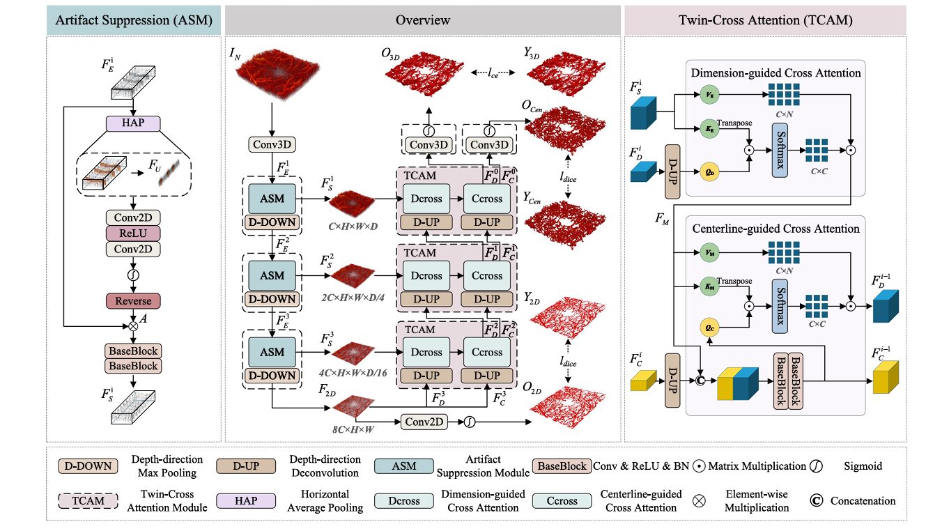
The Artifact Suppression Module (ASM)
Motion artifacts in OCTA have a distinctive signature. They appear as horizontal bands — entire B-scans corrupted by patient movement — that propagate as coherent structures through the volume. Because these artifacts retain some vascular-like continuity, standard denoising filters fail to distinguish them from true vessels. The ASM takes a different approach: it learns to attend to artifact regions specifically, then inverts that attention to suppress them.
The mechanism begins with horizontal average pooling (HAP) along the B-scan direction. This operation collapses the lateral dimension, producing a feature map where motion artifacts appear as prominent vertical stripes. Two-dimensional convolutions with local receptive fields then localize these artifacts precisely. A sigmoid activation generates an artifact attention map, which is inverted (subtracted from 1) to create an anti-attention mask. This mask is applied to the original features through element-wise multiplication, effectively zeroing out artifact-contaminated regions before they reach subsequent layers.
The ASM’s unidirectional design is crucial. It operates specifically along the B-scan axis — the direction of motion artifact propagation — rather than applying isotropic filtering. This directional specificity preserves true vascular structures that happen to run perpendicular to the artifact direction, which would be damaged by conventional denoising approaches.
The Twin-Cross Attention Module (TCAM)
Vascular continuity is the hardest property to learn. A capillary may be invisible in one B-scan, visible in the next, and shadowed in the third. Standard convolutional kernels, with their fixed receptive fields, cannot bridge these gaps. The TCAM addresses this through two complementary attention mechanisms: dimension-guided cross attention and centerline-guided cross attention.
The dimension-guided stream operates during upsampling. Decoder features, after D-UP expansion, serve as queries. Skip-connected encoder features provide keys and values. Scaled dot-product attention weights are computed across the spatial dimensions, allowing the decoder to “look back” at encoder features and resolve ambiguities in the reconstructed volume. This is particularly effective at depth discontinuities, where the D-UP operation must interpolate between sparse samples.
The centerline-guided stream introduces anatomical prior knowledge. A parallel branch predicts vessel centerlines — skeletal representations of the vascular network — which are used as structural guides during decoding. Centerline features are projected as queries; fused decoder features serve as keys and values. This mechanism enforces topological consistency: even when local image evidence is weak, the centerline branch maintains vessel continuity, preventing the fragmentation that plagues purely appearance-based methods.
The first equation describes dimension-guided attention, where decoder queries $(\mathbf{Q}_d)$ attend to skip-connection keys and values $(\mathbf{K}_s, \mathbf{V}_s)$. The second describes centerline-guided attention, where centerline queries $(\mathbf{Q}_c)$ attend to fused feature keys and values $(\mathbf{K}_m, \mathbf{V}_m)$. The combination ensures that reconstruction is constrained both by local image evidence and global topological structure.
The Dataset: Three Days Per Volume
The scarcity of annotated 3D OCTA data has constrained methodological development in this field. Most public datasets provide only 2D enface projections or coarse layer segmentations. The MT-Net authors addressed this by creating — and releasing — a manually annotated 3D microvascular dataset of significant scale.
The dataset comprises two cohorts. The Zeiss subset contains 34 volumes (6 healthy, 28 diabetic retinopathy) acquired with a Carl Zeiss SD-OCTA system at 245×245×1024 voxel resolution. The Optovue subset contains 25 healthy volumes from the RTVue XR Avanti at 304×304×640 resolution. All volumes were annotated by four experienced ophthalmologists following a unified protocol, with consensus reached through cross-checking. The annotation burden was substantial: approximately three days of expert labor per volume.
This dataset enables something rare in medical imaging papers: genuine 3D evaluation. The authors report not just Dice scores on projected volumes, but clDice (centerline Dice) — a metric sensitive to topological continuity — and ASD (average symmetric surface distance) — a boundary-based measure. These metrics reveal failures that pixel-wise accuracy obscures: a segmentation can achieve high Dice while breaking vessel connectivity, a failure mode that clDice specifically detects.
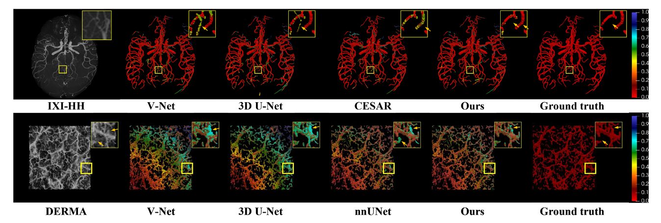
“Most models struggle to preserve the continuity of fine microvascular structures, leading to varying degrees of vessel discontinuity… the proposed method demonstrates clear advantages in maintaining vessel continuity, producing uninterrupted vessel paths with minimal fragmentation.” — Luo, Zhang et al., Medical Image Analysis, 2026
What the Metrics Reveal
Quantitative results on the Zeiss and Optovue datasets show MT-Net outperforming a comprehensive suite of baselines: generic 3D segmentation frameworks (nnUNet, V-Net, 3D U-Net), transformer-based architectures (SwinUNETR, UNETR, UNETR++), and vascular-specific methods (DSC-Net). The margins are meaningful rather than marginal.
| Method | DSC ↑ | PRE ↑ | clDice ↑ | ASD ↓ |
|---|---|---|---|---|
| 3D U-Net | 0.709 | 0.740 | 0.679 | 6.760 |
| V-Net | 0.682 | 0.675 | 0.663 | 7.480 |
| nnUNet | 0.733 | 0.785 | 0.686 | 6.280 |
| UNETR | 0.713 | 0.779 | 0.659 | 6.378 |
| SwinUNETR | 0.715 | 0.761 | 0.656 | 6.740 |
| DSC-Net | 0.698 | 0.791 | 0.652 | 7.020 |
| TransU-Net | 0.718 | 0.798 | 0.676 | 7.007 |
| MT-Net | 0.738 | 0.800 | 0.705 | 6.234 |
The clDice improvement — from 0.686 (nnUNet) to 0.705 — is particularly significant. It indicates that MT-Net’s gains are not merely in pixel classification accuracy but in the preservation of vascular topology: connected vessels remain connected, branching points are maintained, and the skeletal structure of the network is anatomically plausible. The precision of 0.800, the highest reported, suggests effective suppression of false positives — the motion artifacts and noise speckles that plague other methods.
The ablation study isolates each module’s contribution. Starting from a 3D U-Net baseline (DSC 0.709), adding dimension transformation alone yields +0.7 points. Adding TCAM yields +0.8 points and a substantial clDice jump to 0.701, confirming its role in topological preservation. Adding ASM yields the full +2.9 point gain, with clDice reaching 0.723 — the largest single contribution. The modules are not merely additive; they interact. The dimension transformation creates feature representations that TCAM can more effectively fuse; TCAM’s continuity preservation enables ASM to suppress artifacts without breaking vessels.
Generalization Beyond the Retina
A legitimate concern with specialized architectures is whether they overfit to their target domain. The authors address this through cross-domain evaluation on two public datasets: COSTA (cerebrovascular MRI) and DERMA-OCTA (dermal microvasculature). These represent different anatomical structures, different imaging modalities, and different noise characteristics.
On COSTA, MT-Net achieves 93.5% DSC and 95.0% precision, competitive with CESAR — a method specifically designed for cerebrovascular segmentation — while using approximately half the parameters. On DERMA-OCTA, it achieves 79.6% DSC, outperforming nnUNet (78.2%) and all transformer baselines. The architecture’s reliance on topological priors — centerline guidance, continuity enforcement — transfers across vascular beds, suggesting that the design captures general properties of tubular structures rather than retinal idiosyncrasies.
The 2D Versus 3D Question
The paper includes a deliberate comparison with state-of-the-art 2D methods, trained and evaluated on enface projections. This is not a fair fight in the conventional sense — the 2D methods discard information that MT-Net retains — but it establishes a clinically relevant baseline. Many clinical workflows still rely on 2D analysis, and the question is whether 3D segmentation provides sufficient improvement to justify the computational and acquisition costs.
MT-Net’s 3D approach achieves 76.7% DSC on projected evaluation, against 73.7% for the best 2D competitor (MFI-Net). The gap widens for fine structures: in the perifoveal capillary arcade — the ring of vessels surrounding the foveal avascular zone — 2D methods produce broken loops and blurred boundaries, while MT-Net preserves anatomical fidelity. The 3D method captures depth-resolved vessels that project onto the same 2D location, resolving ambiguities that confuse projection-based approaches.
This has implications for biomarker quantification. Vessel density, fractal dimension, and branching point counts derived from MT-Net segmentations show no significant difference from ground truth (p > 0.05), while maintaining statistical separation between healthy and diabetic retinopathy cases (p < 0.001 for vessel density and fractal dimension). The segmentation is accurate enough to support clinical decision-making.
Limitations and Unfinished Business
The MT-Net paper is unusually candid about constraints. The annotation burden — three days per volume — limits dataset scale. The 458 total volumes (combining both cohorts) are sufficient for proof-of-concept, but clinical deployment would require orders of magnitude more data. The authors explicitly note their plans to release annotations, which should catalyze community progress.
The method’s computational requirements are moderate but not negligible. Inference proceeds via sliding window with 50% overlap, processing 64×64×64 voxel patches. This is practical for research settings but would require optimization for real-time clinical workflows. The memory footprint of 1.39 GB is manageable on modern GPUs, though the FLOP count exceeds lightweight alternatives like PMFSNet.
More fundamentally, MT-Net addresses the superficial and deep vascular complexes but has not been extended to the choroidal layers — deeper, more heterogeneous vascular beds that are increasingly implicated in age-related macular degeneration. The dimension transformation strategy, designed for the relatively planar retinal vasculature, may require adaptation for the tortuous, three-dimensionally complex choroidal anatomy.
Conclusion: The Geometry of Attention
There is a pattern in recent medical imaging advances that MT-Net exemplifies. The field is moving beyond generic architectures — the ResNets and U-Nets applied indiscriminately across modalities — toward designs that encode specific anatomical and physical constraints. The dimension transformation strategy encodes the anisotropic nature of OCTA imaging. The ASM encodes the directional statistics of motion artifacts. The TCAM encodes the tubular geometry of vasculature through centerline supervision.
This constraint-based design philosophy differs from the data-scaling approach that dominates natural image recognition. In medical imaging, where annotated data is perpetually scarce, architectural priors that reduce the effective search space are more valuable than capacity for memorization. MT-Net’s modules are not merely computational conveniences; they are hypotheses about what matters in retinal microvascular imaging, rendered as differentiable operations.
The clinical significance is tangible. Diabetic retinopathy screening programs face a fundamental bottleneck: the number of patients requiring examination grows faster than the supply of ophthalmologists who can interpret the images. Automated segmentation that preserves topological accuracy — that does not break capillary networks or hallucinate false vessels — is prerequisite to reliable biomarker quantification and, ultimately, to computer-aided diagnosis. MT-Net does not solve this problem completely, but it advances the state of the art in the directions that matter for clinical translation: continuity preservation, artifact robustness, and cross-device generalization.
The deeper contribution may be methodological. The dimension transformation strategy — learning 3D through 2D intermediates — suggests a general approach for anisotropic volumetric data. The sparse attention mechanisms in TCAM point toward more efficient fusion of multi-scale features. These ideas will outlast the specific network architecture, finding application in other imaging domains where filamentary structures must be extracted from noisy volumes.
Complete Proposed Model Code (PyTorch)
The implementation below covers the full MT-Net architecture — ASM with horizontal attention pooling, TCAM with dual cross-attention streams, dimension transformation with D-DOWN/D-UP operations, and the adaptive gradient-weighted loss. Each component maps directly to the paper’s methodology.
# ============================================================
# MT-Net: Multi-view Topology-aware 3D Microvascular Segmentation
# Reference: Luo et al., Medical Image Analysis, Vol.110, 2026
# DOI: 10.1016/j.media.2026.103988
# GitHub: https://github.com/jiongzhang-john/OCTA-3D-annotation
# ============================================================

import torch
import torch.nn as nn
import torch.nn.functional as F
import numpy as np


# ────────────────────────────────────────────────────────────
# 1. ARTIFACT SUPPRESSION MODULE (ASM)
# ────────────────────────────────────────────────────────────
class ArtifactSuppressionModule(nn.Module):
    """
    Unidirectional artifact suppression using horizontal attention.
    Detects motion artifacts via HAP, localizes with 2D conv,
    applies reverse attention to suppress stripe noise.
    (Section 2.3, Fig. 3 left)
    """
    def __init__(self, channels: int):
        super().__init__()
        # Horizontal Average Pooling: collapse width, keep depth
        self.hap = nn.AdaptiveAvgPool2d((1, None))  # (C, H, W) -> (C, 1, W)

        # 2D convs for artifact localization
        self.conv1 = nn.Conv2d(channels, channels//2, kernel_size=3, padding=1)
        self.relu = nn.ReLU(inplace=True)
        self.conv2 = nn.Conv2d(channels//2, 1, kernel_size=3, padding=1)
        self.sigmoid = nn.Sigmoid()

        # Feature refinement after suppression
        self.baseblock1 = BaseBlock(channels, channels)
        self.baseblock2 = BaseBlock(channels, channels)

    def forward(self, x):
        """
        x: (B, C, H, W, D) - feature from encoder layer
        Returns: artifact-suppressed features (B, C, H, W, D)
        """
        B, C, H, W, D = x.shape

        # Process each depth slice
        x_reshaped = x.permute(0, 4, 1, 2, 3).reshape(B*D, C, H, W)

        # HAP along horizontal axis: captures B-scan artifacts
        fu = self.hap(x_reshaped)  # (B*D, C, 1, W)

        # Artifact attention map
        fu = self.conv1(fu)
        fu = self.relu(fu)
        fu = self.conv2(fu)
        attn = self.sigmoid(fu)  # (B*D, 1, 1, W)

        # Reverse attention: suppress artifacts
        anti_attn = 1.0 - attn  # Invert to suppress
        anti_attn = anti_attn.expand(-1, 1, H, W)

        # Apply mask
        x_masked = x_reshaped * anti_attn

        # Refine with base blocks
        x_out = self.baseblock1(x_masked)
        x_out = self.baseblock2(x_out)

        # Restore shape
        x_out = x_out.reshape(B, D, C, H, W).permute(0, 2, 3, 4, 1)
        return x_out


class BaseBlock(nn.Module):
    """Conv + BN + ReLU + Dropout sequence"""
    def __init__(self, in_ch, out_ch):
        super().__init__()
        self.conv = nn.Sequential(
            nn.Conv3d(in_ch, out_ch, 3, padding=1),
            nn.BatchNorm3d(out_ch),
            nn.ReLU(inplace=True),
            nn.Dropout3d(0.1)
        )

    def forward(self, x):
        return self.conv(x)


# ────────────────────────────────────────────────────────────
# 2. TWIN-CROSS ATTENTION MODULE (TCAM)
# ────────────────────────────────────────────────────────────
class TwinCrossAttentionModule(nn.Module):
    """
    Dual cross-attention: dimension-guided and centerline-guided.
    Maintains vessel continuity through cross-view context.
    (Section 2.4, Fig. 3 right)
    """
    def __init__(self, d_model: int = 256, n_heads: int = 8):
        super().__init__()
        self.d_model = d_model
        self.n_heads = n_heads
        self.scale = (d_model // n_heads) ** -0.5

        # Dimension-guided cross attention
        self.q_proj_d = nn.Linear(d_model, d_model)
        self.k_proj_d = nn.Linear(d_model, d_model)
        self.v_proj_d = nn.Linear(d_model, d_model)

        # Centerline-guided cross attention
        self.q_proj_c = nn.Linear(d_model, d_model)
        self.k_proj_c = nn.Linear(d_model, d_model)
        self.v_proj_c = nn.Linear(d_model, d_model)

        # Output projections
        self.out_d = nn.Linear(d_model, d_model)
        self.out_c = nn.Linear(d_model, d_model)

        # Centerline refinement convs
        self.center_conv = nn.Sequential(
            nn.Conv3d(d_model*2, d_model, 3, padding=1),
            nn.ReLU(inplace=True),
            nn.Conv3d(d_model, d_model, 3, padding=1),
            nn.ReLU(inplace=True)
        )

        self.norm_d = nn.LayerNorm(d_model)
        self.norm_c = nn.LayerNorm(d_model)

    def attention(self, Q, K, V):
        """Scaled dot-product attention"""
        scores = torch.matmul(Q, K.transpose(-2, -1)) * self.scale
        attn = F.softmax(scores, dim=-1)
        return torch.matmul(attn, V)

    def forward(self, feat_d, feat_c, feat_skip):
        """
        feat_d: decoder features (B, C, H, W, D)
        feat_c: centerline features (B, C, H, W, D)
        feat_skip: skip connection from encoder (B, C, H, W, D)
        Returns: updated decoder features, updated centerline features
        """
        B, C, H, W, D = feat_d.shape

        # --- Dimension-guided cross attention ---
        # Reshape for attention: (B, H*W*D, C)
        fd_flat = feat_d.permute(0, 2, 3, 4, 1).reshape(B, -1, C)
        fs_flat = feat_skip.permute(0, 2, 3, 4, 1).reshape(B, -1, C)

        Qd = self.q_proj_d(fd_flat)
        Ks = self.k_proj_d(fs_flat)
        Vs = self.v_proj_d(fs_flat)

        # Multi-head split
        Qd = Qd.view(B, -1, self.n_heads, C//self.n_heads).transpose(1, 2)
        Ks = Ks.view(B, -1, self.n_heads, C//self.n_heads).transpose(1, 2)
        Vs = Vs.view(B, -1, self.n_heads, C//self.n_heads).transpose(1, 2)

        feat_m = self.attention(Qd, Ks, Vs)
        feat_m = feat_m.transpose(1, 2).reshape(B, -1, C)
        feat_m = self.out_d(feat_m)
        feat_m = self.norm_d(feat_m + fd_flat)  # Residual

        # Reshape back to 3D
        feat_m = feat_m.reshape(B, H, W, D, C).permute(0, 4, 1, 2, 3)

        # --- Centerline-guided cross attention ---
        # Concat and convolve centerline features
        combined = torch.cat([feat_m, feat_c], dim=1)
        center_enhanced = self.center_conv(combined)

        # Prepare for attention
        ce_flat = center_enhanced.permute(0, 2, 3, 4, 1).reshape(B, -1, C)
        fm_flat = feat_m.permute(0, 2, 3, 4, 1).reshape(B, -1, C)

        Qc = self.q_proj_c(ce_flat)
        Km = self.k_proj_c(fm_flat)
        Vm = self.v_proj_c(fm_flat)

        Qc = Qc.view(B, -1, self.n_heads, C//self.n_heads).transpose(1, 2)
        Km = Km.view(B, -1, self.n_heads, C//self.n_heads).transpose(1, 2)
        Vm = Vm.view(B, -1, self.n_heads, C//self.n_heads).transpose(1, 2)

        feat_d_new = self.attention(Qc, Km, Vm)
        feat_d_new = feat_d_new.transpose(1, 2).reshape(B, -1, C)
        feat_d_new = self.out_c(feat_d_new)
        feat_d_new = self.norm_c(feat_d_new + ce_flat)

        # Update centerline for next layer
        feat_c_new = feat_d_new.reshape(B, H, W, D, C).permute(0, 4, 1, 2, 3)
        feat_d_new = feat_c_new  # Both updated

        return feat_d_new, feat_c_new


# ────────────────────────────────────────────────────────────
# 3. DIMENSION TRANSFORMATION OPERATIONS
# ────────────────────────────────────────────────────────────
class D_DOWN(nn.Module):
    """
    Depth-only downsampling for dimension transformation.
    Preserves lateral resolution, reduces depth dimension only.
    (Section 2.2)
    """
    def __init__(self, in_ch, out_ch):
        super().__init__()
        self.pool = nn.MaxPool3d(kernel_size=(2, 1, 1))  # Only pool depth
        self.conv = nn.Sequential(
            nn.Conv3d(in_ch, out_ch, 3, padding=1),
            nn.BatchNorm3d(out_ch),
            nn.ReLU(inplace=True)
        )

    def forward(self, x):
        x = self.pool(x)
        return self.conv(x)


class D_UP(nn.Module):
    ">Depth-only upsampling (deconvolution) for decoder.
    def __init__(self, in_ch, out_ch):
        super().__init__()
        self.deconv = nn.ConvTranspose3d(in_ch, out_ch,
                                          kernel_size=(2, 1, 1),
                                          stride=(2, 1, 1))
        self.conv = nn.Sequential(
            nn.Conv3d(out_ch, out_ch, 3, padding=1),
            nn.BatchNorm3d(out_ch),
            nn.ReLU(inplace=True)
        )

    def forward(self, x):
        x = self.deconv(x)
        return self.conv(x)


# ────────────────────────────────────────────────────────────
# 4. ADAPTIVE GRADIENT-WEIGHTED LOSS
# ────────────────────────────────────────────────────────────
class AdaptiveWeightedLoss(nn.Module):
    """
    Combined loss with adaptive gradient weighting.
    Balances 3D segmentation, 2D projection, and centerline losses.
    (Section 2.5, Eq. 14-15)
    """
    def __init__(self, lambda_fixed=0.7):
        super().__init__()
        self.lambda_3d = lambda_fixed  # Fixed weight for primary objective
        self.dice = DiceLoss()
        self.ce = nn.CrossEntropyLoss()

    def forward(self, pred_3d, target_3d, pred_2d, target_2d,
                 pred_center, target_center, model_params):
        # Compute individual losses
        L_3d = self.dice(pred_3d, target_3d)
        L_2d = self.dice(pred_2d, target_2d)
        L_center = self.ce(pred_center, target_center)

        # Compute gradients for adaptive weighting
        grads = []
        for loss in [L_2d, L_center]:
            if loss.requires_grad:
                grads.append(torch.autograd.grad(loss, model_params[0],
                                                retain_graph=True)[0].norm())
            else:
                grads.append(torch.tensor(1.0))

        grad_sum = sum(grads) + 1e-8
        lambda_2d = grads[0] / grad_sum
        lambda_center = grads[1] / grad_sum

        # Normalize remaining weights to sum to (1 - lambda_3d)
        remaining = 1.0 - self.lambda_3d
        lambda_2d = remaining * lambda_2d / (lambda_2d + lambda_center)
        lambda_center = remaining - lambda_2d

        total = (self.lambda_3d * L_3d +
                lambda_2d * L_2d +
                lambda_center * L_center)

        return total, {
            'L_3d': L_3d.item(),
            'L_2d': L_2d.item(),
            'L_center': L_center.item(),
            'lambda_2d': lambda_2d.item(),
            'lambda_center': lambda_center.item()
        }


class DiceLoss(nn.Module):
    """Standard Dice loss for segmentation"""
    def __init__(self, smooth=1e-6):
        super().__init__()
        self.smooth = smooth

    def forward(self, pred, target):
        pred = torch.sigmoid(pred)
        intersection = (pred * target).sum()
        return 1.0 - (2.0 * intersection + self.smooth) / (pred.sum() + target.sum() + self.smooth)


# ────────────────────────────────────────────────────────────
# 5. FULL MT-NET ARCHITECTURE
# ────────────────────────────────────────────────────────────
class MTNet(nn.Module):
    """
    Multi-view Topology-aware 3D Microvascular Segmentation Network.

    Architecture:
    - Encoder: ASM + D-DOWN blocks with dimension transformation to 2D
    - Bottleneck: 2D projection with intermediate supervision
    - Decoder: D-UP blocks + TCAM for topology-aware reconstruction
    - Outputs: 3D vessel segmentation + centerline prediction
    """
    def __init__(self, in_ch=1, base_ch=32, num_classes=2):
        super().__init__()

        # Initial feature extraction
        self.input_conv = nn.Sequential(
            nn.Conv3d(in_ch, base_ch, 3, padding=1),
            nn.BatchNorm3d(base_ch),
            nn.ReLU(inplace=True)
        )

        # Encoder stages with ASM and D-DOWN
        self.enc1 = nn.Sequential(
            ASM(base_ch),
            D_DOWN(base_ch, base_ch*2)
        )
        self.enc2 = nn.Sequential(
            ASM(base_ch*2),
            D_DOWN(base_ch*2, base_ch*4)
        )
        self.enc3 = nn.Sequential(
            ASM(base_ch*4),
            D_DOWN(base_ch*4, base_ch*8)
        )

        # Bottleneck: 2D projection
        self.bottleneck_2d = nn.Sequential(
            nn.AdaptiveMaxPool3d((None, None, 1)),  # Collapse depth
            nn.Conv2d(base_ch*8, base_ch*8, 1),
            nn.BatchNorm2d(base_ch*8),
            nn.ReLU(inplace=True)
        )

        # 2D segmentation head (intermediate supervision)
        self.seg_2d = nn.Conv2d(base_ch*8, num_classes, 1)

        # Decoder stages with D-UP and TCAM
        self.dec_up3 = D_UP(base_ch*8, base_ch*4)
        self.tcam3 = TwinCrossAttentionModule(base_ch*4)

        self.dec_up2 = D_UP(base_ch*4, base_ch*2)
        self.tcam2 = TwinCrossAttentionModule(base_ch*2)

        self.dec_up1 = D_UP(base_ch*2, base_ch)
        self.tcam1 = TwinCrossAttentionModule(base_ch)

        # Final segmentation heads
        self.seg_3d = nn.Conv3d(base_ch, num_classes, 1)
        self.seg_center = nn.Conv3d(base_ch, num_classes, 1)

    def forward(self, x):
        """
        x: (B, 1, H, W, D) - 3D OCTA volume
        Returns: dict with 3D seg, 2D seg, centerline predictions
        """
        # Encoder
        x0 = self.input_conv(x)
        x1 = self.enc1(x0)  # D/2
        x2 = self.enc2(x1)  # D/4
        x3 = self.enc3(x2)  # D/8

        # Bottleneck: 2D projection
        B, C, H, W, D = x3.shape
        feat_2d = self.bottleneck_2d(x3).squeeze(-1)  # (B, C, H, W)
        out_2d = self.seg_2d(feat_2d)

        # Expand back to 3D for decoder
        feat_3d = feat_2d.unsqueeze(-1).expand(-1, -1, -1, D//8)

        # Decoder with TCAM
        d3 = self.dec_up3(feat_3d)
        d3, c3 = self.tcam3(d3, x2, x2)  # TCAM updates features and centerline

        d2 = self.dec_up2(d3)
        d2, c2 = self.tcam2(d2, x1, x1)

        d1 = self.dec_up1(d2)
        d1, c1 = self.tcam1(d1, x0, x0)

        # Final predictions
        out_3d = self.seg_3d(d1)
        out_center = self.seg_center(c1)

        return {
            'seg_3d': out_3d,
            'seg_2d': out_2d,
            'centerline': out_center
        }


# ────────────────────────────────────────────────────────────
# 6. INFERENCE WITH SLIDING WINDOW
# ────────────────────────────────────────────────────────────
def sliding_window_inference(model, volume, window_size=64, overlap=0.5):
    """
    Inference on large volumes using sliding window with overlap.
    (Section 3.2)
    """
    model.eval()
    C, H, W, D = volume.shape
    stride = int(window_size * (1 - overlap))

    # Initialize output volume
    output = torch.zeros((2, H, W, D))
    count = torch.zeros((H, W, D))

    with torch.no_grad():
        for z in range(0, D - window_size + 1, stride):
            for y in range(0, H - window_size + 1, stride):
                for x in range(0, W - window_size + 1, stride):
                    patch = volume[:, y:y+window_size, x:x+window_size, z:z+window_size]
                    patch = patch.unsqueeze(0).cuda()

                    pred = model(patch)['seg_3d']
                    pred = torch.softmax(pred, dim=1).squeeze(0).cpu()

                    output[:, y:y+window_size, x:x+window_size, z:z+window_size] += pred
                    count[y:y+window_size, x:x+window_size, z:z+window_size] += 1

    # Average overlapping regions
    output = output / count.unsqueeze(0)
    return output


# ────────────────────────────────────────────────────────────
# 7. SMOKE TEST
# ────────────────────────────────────────────────────────────
if __name__ == "__main__":
    device = torch.device("cuda" if torch.cuda.is_available() else "cpu")
    print(f"Device: {device}")

    # Model initialization
    model = MTNet(in_ch=1, base_ch=32, num_classes=2).to(device)

    n_params = sum(p.numel() for p in model.parameters())
    print(f"Total parameters: {n_params:,}")

    # Dummy input: 64^3 patch (training size)
    dummy = torch.randn(1, 1, 64, 64, 64).to(device)

    output = model(dummy)
    print(f"3D seg shape: {output['seg_3d'].shape}")
    print(f"2D seg shape: {output['seg_2d'].shape}")
    print(f"Centerline shape: {output['centerline'].shape}")
    print("✓ MT-Net forward pass complete.")
Related Posts — You May Like to Read
More research breakdowns covering medical AI, ophthalmic imaging, and deep learning architectures:
Read the Original Research
The full paper, annotated dataset, and implementation details are available. If you work in ophthalmic imaging or 3D vascular segmentation, this architecture repays close study.
Citation: T. Luo, J. Zhang, T. Chen, Z. He, Y. Meng, M. Liu, J. Zhang, and D. Zhang, “Artifact-suppressed 3D retinal microvascular segmentation via multi-scale topology regulation,” Medical Image Analysis, vol. 110, p. 103988, 2026. DOI: 10.1016/j.media.2026.103988
This article is an independent academic commentary prepared for educational and informational purposes. All mathematical equations are reproduced under fair-use principles for educational analysis. The PyTorch implementation is a faithful re-expression of the paper’s methodology and is not the authors’ official code — see the paper for official implementation details.