SSA-Mamba: The Hyperspectral Classifier That Finally Lets Spatial and Spectral Features Talk to Each Other
Researchers at Guangzhou Maritime University diagnosed a fundamental flaw in every existing hyperspectral classification model — spatial and spectral features are either forced to share the same representation space, or kept so separate they never productively interact. SSA-Mamba fixes both problems at once: dual branches with independent parameters prevent coupling, while asymmetric cross-domain attention lets spatial features actively query spectral information. The result is state-of-the-art accuracy on all three benchmark datasets, a 21× memory reduction versus the competition, and the ability to run on 5.92 million pixel images that Transformer methods literally cannot fit in GPU memory.
Hyperspectral cameras capture hundreds of wavelength bands simultaneously — a satellite flying over a wheat field sees not just visible color but near-infrared absorption curves for every 30-centimeter patch of soil. Classifying every pixel in that image into meaningful land cover categories (healthy crop versus stressed crop versus bare soil versus road) is one of the hardest perception problems in remote sensing. The core difficulty is that you need both: spectral uniqueness (this pixel’s absorption signature matches cotton, not rape) and spatial context (this cluster of pixels forms a field boundary, not a random noise patch). Getting both, efficiently, without one corrupting the other, is what SSA-Mamba finally gets right.
What Every Previous Method Got Wrong
The history of hyperspectral image classification is a sequence of partial fixes to a problem nobody had fully diagnosed. CNNs gave you spatial patterns but constrained you to local receptive fields — if your target category only makes sense in the context of its distant neighbors, convolution misses it. Transformers gave you global attention but came with quadratic memory complexity, which means on the XiongAn dataset (1,580 × 3,750 pixels = nearly 6 million spatial positions), two of the three Transformer baselines in this paper literally ran out of GPU memory on a 24GB RTX 4090 and could not produce results at all.
Mamba-based SSMs fixed the complexity problem with O(L) linear scaling through recursive state updates. But existing SSM approaches for hyperspectral data had their own structural flaw: they processed spatial and spectral information either in the same branch (feature coupling — the model has to use the same parameters to learn both geometric patterns and absorption signatures, which are physically very different phenomena) or in completely separate branches with no interaction (feature isolation — you have two expert opinions but no meeting room). The paper quantifies what coupling costs: for spectrally similar Brassica crop varieties on the WHU-Hi-HongHu dataset, coupled-feature approaches achieve roughly 50-60% classification accuracy on the hardest categories. SSA-Mamba’s dual-branch design with cross-domain interaction lifts this to 73-82%.
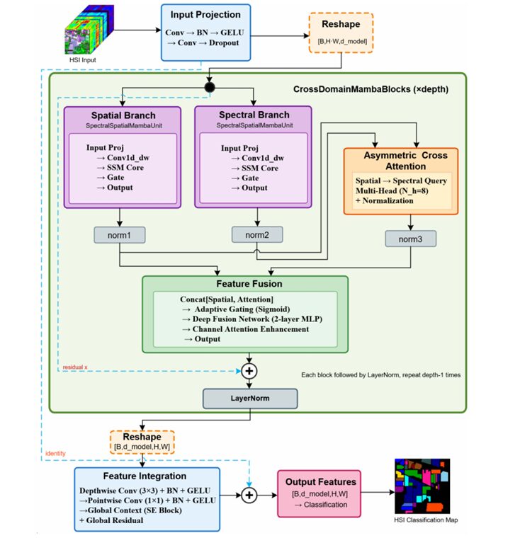
SSA-Mamba uses two completely independent SSM branches — separate weights, separate parameters — for spatial and spectral processing. This prevents the interference of physically distinct feature types. But rather than keeping them isolated, an asymmetric cross-domain attention module lets spatial features actively query spectral information (not the other way around), establishing a one-directional information flow that the ablation study shows outperforms symmetric bidirectional attention by 1.66 percentage points while using fewer parameters.
The Full SSA-Mamba Architecture
INPUT: HSI Patch X ∈ R^(B × C × H × W)
  C = spectral bands (up to 270), H×W = spatial patch (7×7 default)
         │
┌────────▼──────────────────────────────────────────────────────────┐
│  INPUT PROJECTION MODULE                                          │
│    1×1 Conv (C → d_model/2) → BatchNorm → GELU                   │
│    3×3 Conv (d_model/2 → d_model) → BatchNorm → GELU → Dropout   │
│  → Z_proj ∈ R^(B × d_model × H × W)                              │
│  Reshape → Z_seq ∈ R^(B × L × d_model)   [L = H×W sequence]     │
└────────┬──────────────────────────────────────────────────────────┘
         │  (repeat depth=4 times)
┌────────▼──────────────────────────────────────────────────────────┐
│  CROSSDOMAINMAMBABLOCK (×depth)                                   │
│                                                                    │
│  ┌─────────────────────┐  ┌─────────────────────┐                 │
│  │  SPATIAL BRANCH     │  │  SPECTRAL BRANCH     │                 │
│  │  (Θ_spatial params) │  │  (Θ_spectral params) │                │
│  │                     │  │                      │                 │
│  │  Input Proj         │  │  Input Proj          │                 │
│  │  x → Win → LN       │  │  x → Win → LN        │                │
│  │  → split main/gate  │  │  → split main/gate   │                │
│  │                     │  │                      │                 │
│  │  Conv1d_depthwise   │  │  Conv1d_depthwise    │                 │
│  │  (local correlation)│  │  (local correlation) │                 │
│  │                     │  │                      │                 │
│  │  SSM Core:          │  │  SSM Core:           │                 │
│  │  Δ = exp(Δ_log)     │  │  Δ = exp(Δ_log)      │                │
│  │  A = -exp(A_log)    │  │  A = -exp(A_log)     │                │
│  │  Ā = exp(Δ⊙A)      │  │  Ā = exp(Δ⊙A)       │                │
│  │  B̄ = Δ⊙B           │  │  B̄ = Δ⊙B            │                │
│  │  h_t = h_{t-1}⊙Ā   │  │  h_t = h_{t-1}⊙Ā    │                │
│  │      + x_t⊙B̄       │  │      + x_t⊙B̄        │                │
│  │  y_t = ⟨h_t,C⟩+x⊙D │  │  y_t = ⟨h_t,C⟩+x⊙D  │               │
│  │                     │  │                      │                 │
│  │  Gate: y⊙SiLU(gate) │  │  Gate: y⊙SiLU(gate)  │               │
│  │  + LayerNorm + Res  │  │  + LayerNorm + Res   │                 │
│  └──────────┬──────────┘  └──────────┬───────────┘                │
│             │ f_spatial              │ f_spectral                  │
│             │ LayerNorm1             │ LayerNorm2                  │
│             │                        │                             │
│  ┌──────────▼────────────────────────▼───────────┐                │
│  │  ASYMMETRIC CROSS-DOMAIN ATTENTION            │                │
│  │  Q = f_spatial (spatial queries spectral!)    │                │
│  │  K = V = f_spectral                           │                │
│  │  8 parallel attention heads (d_h = d/N_h)    │                │
│  │  A_i = softmax(Q_i K_i^T / √d_h)             │                │
│  │  head_i = A_i · V_i                           │                │
│  │  f_attn = LayerNorm3(Concat(heads)·W_O)       │                │
│  └──────────────────────┬────────────────────────┘                │
│                          │                                         │
│  ┌───────────────────────▼────────────────────────┐               │
│  │  FEATURE FUSION MODULE                         │               │
│  │  f_concat = [f_spatial ; f_attn]               │               │
│  │  g = σ(f_concat · W_g + b_g)   [gating]       │               │
│  │  f_fuse = MLP(LayerNorm(f_concat))             │               │
│  │  f_fuse = f_fuse ⊙ g           [gated select] │               │
│  │  Channel Attention (SE Block):                 │               │
│  │    w = σ(Conv(ReLU(Conv(AvgPool(f_fuse)))))   │               │
│  │    f_ca = f_fuse ⊙ w                           │               │
│  │  Block Residual: LayerNorm(f_ca + x_input)     │               │
│  └───────────────────────┬────────────────────────┘               │
└────────────────────────┬─┘                                        │
                         │ (after depth blocks)                      │
┌────────────────────────▼──────────────────────────────────────────┐
│  FEATURE INTEGRATION MODULE                                       │
│  Reshape Z_blocks → [B, d_model, H, W]                           │
│  Depthwise Conv 3×3 + BN + GELU                                   │
│  Pointwise Conv 1×1 + BN + GELU + Dropout2d                       │
│  SE Block (Global Context): AvgPool → Conv → ReLU → Conv → σ     │
│  Global Residual: Z_final = Z_enhanced + Z_proj   ← shallow fuse  │
└────────────────────────┬──────────────────────────────────────────┘
                         │
                    GlobalAvgPool2d
                         │
                    Linear Classifier
                         │
              p = softmax(Z · W_cls + b_cls)
Module 1: The SpectralSpatialMambaUnit
Why Independent Parameters Matter
The spatial branch and spectral branch in SSA-Mamba are both instances of the same class — SpectralSpatialMambaUnit — but they have entirely separate weight matrices. There is no sharing. This is deliberate: spatial patterns (field boundaries, building edges, road networks) are primarily about geometric relationships between adjacent pixels. Spectral patterns (absorption curves distinguishing healthy from stressed vegetation) are primarily about the shape of the wavelength response curve at a single pixel. These are different physical phenomena that require different learned transformations, and forcing a single set of weights to model both leads to feature coupling that degrades accuracy on spectrally similar categories.
Exponential Parameterization for Numerical Stability
The SSM core defines five learnable parameter sets. The critical design choice for stable training is exponential parameterization of the two that need constrained ranges: the step size Δ and the state transition matrix A.
The exponential ensures Δ is always positive (valid step sizes). The negative exponential guarantees A’s eigenvalues are always negative — a mathematical requirement for system stability that prevents the hidden state from exploding. Parameters are learned in log-space, where gradients are well-conditioned, and mapped to computation-space via exp. The paper notes this was essential for avoiding gradient explosion during training with depth-4 networks.
The Recursive State Update
For each time step t in the serialized spatial sequence (where sequence position maps to spatial location via row-major ordering i = h×W + w):
The first term carries historical state with exponential decay. The second injects the current input. The skip connection D·x lets raw input flow directly to output without passing through the state — critical for gradient flow in deep stacks. The result: each position’s output depends on the entire preceding sequence, giving O(L) global receptive field without O(L²) attention cost.
Module 2: Asymmetric Cross-Domain Attention
Spatial Queries Spectral — Not the Other Way Around
This is the design decision the ablation study most clearly validates. In the cross-domain attention module, the Query comes from spatial features and the Key/Value come from spectral features. The direction is intentional: spatial features are asking “what spectral signature is at the locations I’m paying attention to?” The model learns to use spatial context (where am I, what are my geometric neighbors?) to selectively retrieve the most informative spectral information.
The ablation table is unambiguous: replacing the asymmetric design with symmetric bidirectional attention (where both branches query each other) drops OA from 93.98% to 92.32% on Houston2013, a 1.66 percentage point loss despite using more parameters. Spatial-to-spectral querying captures the directional relationship correctly. Allowing spectral features to query spatial features adds noise without adding signal for land cover classification.
Module 3: Adaptive Feature Fusion
After the attention module, the spatial features and attended spectral features are fused through three mechanisms working together. First, a gating network produces a per-channel sigmoid weight vector from the concatenated features — letting the model learn, for each scene, how much to trust spatial versus attended-spectral signals. Second, a two-layer MLP with LayerNorm performs deep non-linear fusion of the gated features. Third, a Squeeze-and-Excitation channel attention block recalibrates the importance of each of the 256 feature channels globally, using adaptive average pooling followed by two 1×1 convolutions.
The ablation results show the gating mechanism contributes 1.62 percentage points of OA improvement on its own. Removing it drops accuracy from 93.98% to 92.36%. The multiscale residual connections (the block-internal residual adding the original input back after fusion) contribute even more — removing multiscale features causes a 2.41 percentage point drop, the single largest ablation loss in the study.
“For spectrally confused categories pakchoi, romaine lettuce, and carrot, SSA-Mamba surpassed second-best methods by 8.38%, 8.35%, and 4.06 percentage points respectively, fully demonstrating the robustness of cross-domain attention fusion mechanisms in handling spectrally confused categories.” — Liao & Wang, IEEE JSTARS, Vol. 19, 2026
Results: Three Datasets, Three Different Stories
Houston2013 — Urban Land Cover With Spectrally Similar Grass
| Method | OA (%) | AA (%) | Kappa |
|---|---|---|---|
| CNN | 88.47 | 88.05 | 87.52 |
| ResNet | 89.38 | 88.59 | 88.51 |
| ATN-hybrid | 92.71 | 93.36 | 92.12 |
| SpecSpatMamba | 89.97 | 90.62 | 89.16 |
| DualPathMamba | 92.24 | 92.95 | 91.60 |
| SSA-Mamba (ours) | 93.98 | 94.72 | 93.49 |
The standout result on Houston2013 is the Highway category: SSA-Mamba achieves 98.24% accuracy versus the second-best ATN-hybrid’s 82.58% — a 15.66 percentage point improvement. Highways are spectrally ambiguous (asphalt looks similar to parking lots and roads) but spatially distinctive (long linear structures with specific neighborhood topology). This is exactly the scenario where spatial-features-querying-spectral-information shines.
WHU-Hi-HongHu — 22 Crop Types, Extreme Spectral Similarity
| Category | CNN | ATN-hybrid | SSA-Mamba | Improvement vs. CNN |
|---|---|---|---|---|
| Brassica parachinensis | 59.32 | — | 78.53 | +19.21 pp |
| Brassica chinensis | 50.55 | — | 73.88 | +23.33 pp |
| Small Brassica chinensis | 85.78 | — | 82.47 | — |
| Pakchoi | 12.56 | 42.02 | 50.40 | +8.38 pp vs. 2nd |
| Cotton | — | — | 99.61 | — |
| Overall (OA) | 88.60 | 93.33 | 93.58 | +0.25 pp vs. 2nd |
XiongAn — 5.92 Million Pixels, Where Transformers Crash
| Method | OA (%) | Peak GPU Memory | Params (M) | Inference (ms) |
|---|---|---|---|---|
| MetaFormer-T | OOM — Cannot run (>24 GB) | — | ||
| ConTNet-T | OOM — Cannot run (>24 GB) | — | ||
| SpecSpatMamba | 93.44 | 3,015 MB | 157.23 | — |
| ATN-hybrid | 94.79 | — | — | — |
| DualPathMamba | 96.25 | — | — | — |
| SSA-Mamba (ours) | 96.06 | 317 MB | 7.32 | 0.646 |
The XiongAn numbers tell two separate stories. The accuracy story: SSA-Mamba is competitive with DualPathMamba (96.06% vs 96.25%) and significantly ahead of all other methods. The efficiency story: SSA-Mamba uses 317 MB of GPU memory versus SpecSpatMamba’s 3,016 MB — a 9.5× reduction — and 95.7% less than MetaFormer-T (7,322 MB). With only 7.32 million parameters versus SpecSpatMamba’s 157 million, SSA-Mamba demonstrates that architectural inductive biases (dual-branch decoupling, asymmetric attention, hierarchical residuals) contribute more to accuracy than raw parameter count.
Complete End-to-End SSA-Mamba Implementation (PyTorch)
The implementation covers every component from the paper in 12 sections: the exponential-parameterized SSM core with ZOH discretization, the complete SpectralSpatialMambaUnit with depthwise convolution and gating, the asymmetric cross-domain attention module with 8 parallel heads, the adaptive feature fusion with gating and SE channel attention, the CrossDomainMambaBlock with three-level residual connections, the input projection and serialization module, the feature integration module with global SE context, the full SSA-Mamba classifier, dataset utilities for patch-based HSI processing, the complete training loop with cosine annealing, and an end-to-end smoke test.
# ==============================================================================
# SSA-Mamba: Spatial-Spectral Attentive State Space Model
# Paper: IEEE JSTARS Vol.19, 2026 — DOI: 10.1109/JSTARS.2026.3654346
# Authors: Jianshang Liao, Liguo Wang
# Affiliation: Guangzhou Maritime University / Dalian Minzu University
# ==============================================================================
# Sections:
# 1. Imports & Configuration
# 2. SSM Core with Exponential Parameterization (Eq. 6-10)
# 3. SpectralSpatialMambaUnit (full SSM layer, Eq. 3-12)
# 4. Asymmetric Cross-Domain Attention (Eq. 15-19)
# 5. SE Channel Attention Block (Eq. 24-26)
# 6. Feature Fusion Module (Eq. 20-27)
# 7. CrossDomainMambaBlock (full dual-branch block, Eq. 13-27)
# 8. Input Projection & Serialization Module (Eq. 1-2)
# 9. Feature Integration Module (Eq. 29-34)
# 10. SSA-Mamba Classifier (full model, Algorithm 1)
# 11. HSI Dataset Utilities (patch extraction, data loading)
# 12. Training Loop & Smoke Test
# ==============================================================================
from __future__ import annotations
import math
import warnings
from dataclasses import dataclass
from typing import Optional, Tuple
import torch
import torch.nn as nn
import torch.nn.functional as F
from torch import Tensor
warnings.filterwarnings("ignore")
# ─── SECTION 1: Configuration ─────────────────────────────────────────────────
@dataclass
class SSAMambaConfig:
"""
SSA-Mamba hyperparameters. Default values match the paper's
best configuration (validated on Houston2013, WHU-Hi-HongHu, XiongAn).
"""
# Input
in_channels: int = 144 # spectral bands (144 for Houston2013)
patch_size: int = 7 # spatial neighborhood (7×7)
n_classes: int = 15 # number of land cover categories
# Core architecture
d_model: int = 256 # hidden dimension (paper default)
d_state: int = 16 # SSM state dimension (paper default)
d_conv: int = 3 # depthwise conv kernel size
expand: int = 2 # expansion ratio (d_inner = expand × d_model)
depth: int = 4 # number of CrossDomainMambaBlocks
n_heads: int = 8 # attention heads in cross-domain module
# Regularization
dropout: float = 0.1 # dropout rate throughout
@property
def d_inner(self) -> int:
return self.expand * self.d_model
@property
def d_head(self) -> int:
return self.d_model // self.n_heads
@property
def seq_len(self) -> int:
return self.patch_size * self.patch_size
# ─── SECTION 2: SSM Core with Exponential Parameterization ────────────────────
class SSMCore(nn.Module):
"""
State Space Model core with ZOH discretization (Eq. 6-10).
Learnable parameters and their roles:
Δ_log ∈ R^d_inner : controls state update rate (step size)
A_log ∈ R^(d_inner × d_state) : historical information decay
B ∈ R^(d_inner × d_state) : input influence on state
C ∈ R^(d_inner × d_state) : state-to-output mapping
D ∈ R^d_inner : skip connection (direct input→output)
Exponential Parameterization (Eq. 7):
Δ = exp(Δ_log) → always positive step size
A = -exp(A_log) → always negative eigenvalues → system stability
ZOH Discretization (Eq. 8):
Ā = exp(Δ ⊙ A) → discrete state transition
B̄ = Δ ⊙ B → discrete input matrix
Recursive State Update (Eq. 9-10):
h_t = h_{t-1} ⊙ Ā + x_t ⊙ B̄
y_t = ⟨h_t, C⟩ + x_t ⊙ D
Complexity: O(L · d_inner · d_state) — linear in sequence length
"""
def __init__(self, d_inner: int, d_state: int):
super().__init__()
self.d_inner = d_inner
self.d_state = d_state
# Learnable parameters in log space for numerical stability
self.delta_log = nn.Parameter(torch.zeros(d_inner))
self.A_log = nn.Parameter(torch.log(torch.rand(d_inner, d_state) + 0.1))
self.B = nn.Parameter(torch.randn(d_inner, d_state) * 0.02)
self.C = nn.Parameter(torch.randn(d_inner, d_state) * 0.02)
self.D = nn.Parameter(torch.ones(d_inner)) # skip connection
def forward(self, x: Tensor) -> Tensor:
"""
x: (B, L, d_inner) — input sequence (serialized spatial positions)
Returns y: (B, L, d_inner) — output with global dependency
"""
B_sz, L, D = x.shape
# Eq. 7: Exponential parameterization
delta = F.softplus(self.delta_log) # (d_inner,) always positive
A = -torch.exp(self.A_log.float()) # (d_inner, d_state) always negative
# Eq. 8: ZOH discretization
# Ā = exp(Δ ⊙ A): (d_inner, d_state)
A_bar = torch.exp(delta.unsqueeze(-1) * A)
# B̄ = Δ ⊙ B: (d_inner, d_state)
B_bar = delta.unsqueeze(-1) * self.B
# Eq. 9-10: Sequential state recursion
# h ∈ R^(B, d_inner, d_state)
h = torch.zeros(B_sz, D, self.d_state, device=x.device, dtype=x.dtype)
ys = []
for t in range(L):
x_t = x[:, t, :] # (B, d_inner)
# h_t = h_{t-1} ⊙ Ā + x_t ⊙ B̄
h = h * A_bar.unsqueeze(0) + x_t.unsqueeze(-1) * B_bar.unsqueeze(0)
# y_t = ⟨h_t, C⟩ + x_t ⊙ D
y_t = (h * self.C.unsqueeze(0)).sum(dim=-1) + x_t * self.D
ys.append(y_t)
return torch.stack(ys, dim=1) # (B, L, d_inner)
# ─── SECTION 3: SpectralSpatialMambaUnit ──────────────────────────────────────
class SpectralSpatialMambaUnit(nn.Module):
"""
Core SSM processing unit used in both spatial and spectral branches.
Pipeline (paper Section II-C and Algorithm function block):
1. Input projection: x → LayerNorm → Linear → [main | gate] split
2. Depthwise conv on main path (local temporal correlation)
3. SSM core (global dependency with linear complexity)
4. Gating: y_gated = y ⊙ SiLU(gate) [adaptive information flow]
5. Output projection + residual connection
The key: spatial branch (Θ_spatial) and spectral branch (Θ_spectral)
each instantiate this class with COMPLETELY SEPARATE parameters.
No weight sharing. Each branch learns domain-specific representations.
"""
def __init__(self, d_model: int, d_state: int, d_conv: int, expand: int, dropout: float):
super().__init__()
d_inner = expand * d_model
# Step 1: Input projection → expand + split into main + gate
self.norm_in = nn.LayerNorm(d_model)
self.in_proj = nn.Linear(d_model, 2 * d_inner) # outputs [main; gate]
# Step 2: Depthwise separable conv on main path (Eq. 5)
# Operates on (B, d_inner, L), extracts local correlations
self.conv1d = nn.Conv1d(
in_channels=d_inner,
out_channels=d_inner,
kernel_size=d_conv,
padding=d_conv - 1,
groups=d_inner, # depthwise: each channel independent
)
self.conv_bn = nn.BatchNorm1d(d_inner)
self.conv_act = nn.SiLU()
# Step 3: SSM core (global long-range dependency)
self.ssm = SSMCore(d_inner, d_state)
# Step 5: Output projection with dropout
self.out_proj = nn.Linear(d_inner, d_model)
self.dropout = nn.Dropout(dropout)
self.norm_out = nn.LayerNorm(d_model)
def forward(self, x: Tensor) -> Tensor:
"""
x: (B, L, d_model) — input sequence
Returns: (B, L, d_model) — transformed sequence with residual
"""
B, L, _ = x.shape
residual = x
# Step 1: LayerNorm + linear projection + split
h_proj = self.in_proj(self.norm_in(x)) # (B, L, 2*d_inner)
h_main, h_gate = h_proj.chunk(2, dim=-1) # each (B, L, d_inner)
# Step 2: Depthwise conv on main path — (B, d_inner, L) format
# Eq. 5: h_conv = SiLU(BN(Conv1d_dw(h_main^T)))^T
h_t = h_main.transpose(1, 2) # (B, d_inner, L)
h_t = self.conv1d(h_t)[..., :L] # trim padding
h_conv = self.conv_act(self.conv_bn(h_t)).transpose(1, 2) # (B, L, d_inner)
# Step 3: SSM core — global dependency modeling
y = self.ssm(h_conv) # (B, L, d_inner)
# Step 4: Gating mechanism (Eq. 11)
y_gated = y * F.silu(h_gate) # (B, L, d_inner)
# Step 5: Output projection + residual (Eq. 12)
out = self.dropout(self.out_proj(y_gated))
return self.norm_out(out + residual) # (B, L, d_model)
# ─── SECTION 4: Asymmetric Cross-Domain Attention ─────────────────────────────
class AsymmetricCrossDomainAttention(nn.Module):
"""
Asymmetric cross-domain attention (Section II-D, Eq. 15-19).
Spatial features serve as Query — they actively query spectral info.
Spectral features serve as Key and Value — they are queried.
Why asymmetric? Physical reasoning:
- Spatial features know WHERE (geometric context, boundaries)
- Spectral features know WHAT (material absorption signatures)
- Asking "what spectral info is relevant to my spatial context?"
is more meaningful than the reverse.
Ablation validation: asymmetric (93.98% OA) > symmetric (92.32% OA)
with fewer parameters, confirming the directional design.
Multi-head attention with N_h=8 heads, d_h = d_model / N_h = 32.
Each head learns different spatial-spectral correspondence patterns.
"""
def __init__(self, d_model: int, n_heads: int):
super().__init__()
assert d_model % n_heads == 0, "d_model must be divisible by n_heads"
self.n_heads = n_heads
self.d_head = d_model // n_heads
self.scale = self.d_head ** -0.5
# Per-head projections for Q (from spatial), K, V (from spectral)
self.W_Q = nn.Linear(d_model, d_model, bias=False) # Query from spatial
self.W_K = nn.Linear(d_model, d_model, bias=False) # Key from spectral
self.W_V = nn.Linear(d_model, d_model, bias=False) # Value from spectral
self.W_O = nn.Linear(d_model, d_model, bias=False) # Output projection
self.norm = nn.LayerNorm(d_model)
def forward(self, f_spatial: Tensor, f_spectral: Tensor) -> Tensor:
"""
f_spatial: (B, L, d_model) — from spatial SSM branch (→ Query)
f_spectral: (B, L, d_model) — from spectral SSM branch (→ Key, Value)
Returns: (B, L, d_model) — attended features with LayerNorm
"""
B, L, D = f_spatial.shape
H, Dh = self.n_heads, self.d_head
# Eq. 15: Asymmetric Q-K-V assignment
Q = self.W_Q(f_spatial) # (B, L, D) — spatial queries spectral
K = self.W_K(f_spectral) # (B, L, D) — spectral keys
V = self.W_V(f_spectral) # (B, L, D) — spectral values
# Reshape for multi-head: (B, H, L, Dh)
Q = Q.view(B, L, H, Dh).transpose(1, 2)
K = K.view(B, L, H, Dh).transpose(1, 2)
V = V.view(B, L, H, Dh).transpose(1, 2)
# Eq. 17: Attention weights A_i = softmax(Q_i K_i^T / sqrt(d_h))
attn = (Q @ K.transpose(-2, -1)) * self.scale # (B, H, L, L)
attn = F.softmax(attn, dim=-1)
# Eq. 18: Value aggregation — head_i = A_i · V_i
out = (attn @ V).transpose(1, 2).reshape(B, L, D) # (B, L, D)
# Eq. 19: Output projection + LayerNorm
out = self.W_O(out)
return self.norm(out) # f_attn_norm
# ─── SECTION 5: SE Channel Attention Block ────────────────────────────────────
class SEChannelAttention(nn.Module):
"""
Squeeze-and-Excitation channel attention (Eq. 24-26).
Global statistical information via average pooling, then learned
nonlinear dependencies between channels through a 2-layer FC network.
This adaptively recalibrates which of the 256 feature channels matter
most for the current scene — key for distinguishing subtle spectral features.
f_pool = AdaptiveAvgPool1d(f^T)
w_channel = σ(Conv1×1(ReLU(Conv1×1(f_pool))))
f_ca = f ⊙ w_channel
"""
def __init__(self, d_model: int, reduction: int = 16):
super().__init__()
d_reduced = max(d_model // reduction, 4)
self.fc1 = nn.Linear(d_model, d_reduced)
self.fc2 = nn.Linear(d_reduced, d_model)
def forward(self, x: Tensor) -> Tensor:
"""
x: (B, L, d_model)
Returns: (B, L, d_model) — channel-recalibrated features
"""
# Eq. 24: Global average pool over sequence dimension
pool = x.mean(dim=1) # (B, d_model)
# Eq. 25: Two-layer channel attention with ReLU + sigmoid
w = F.relu(self.fc1(pool)) # (B, d_reduced)
w = torch.sigmoid(self.fc2(w)) # (B, d_model)
# Eq. 26: Channel-wise recalibration
return x * w.unsqueeze(1) # (B, L, d_model) broadcast
# ─── SECTION 6: Feature Fusion Module ────────────────────────────────────────
class FeatureFusionModule(nn.Module):
"""
Adaptive feature fusion (Section II-D, Eq. 20-27).
Combines spatial features and cross-attended spectral features
through three complementary mechanisms:
1. Gating (Eq. 21-23):
g = σ(f_concat · W_g) [per-channel sigmoid gate]
f_fused = MLP(f_concat) ⊙ g [selective activation]
2. Deep Fusion Network (Eq. 22):
Two-layer MLP with LayerNorm, GELU, and Dropout
3. Channel Attention Enhancement (Eq. 24-26):
SE block recalibrates channel importance globally
Ablation results:
- Removing gating: -1.62 pp OA (92.36% vs 93.98%)
- Removing multiscale residuals: -2.41 pp OA (91.57% vs 93.98%)
"""
def __init__(self, d_model: int, dropout: float):
super().__init__()
d_concat = 2 * d_model # concatenated spatial + attention features
# Gating network
self.gate_proj = nn.Linear(d_concat, d_model)
# Deep fusion MLP (2-layer with intermediate LayerNorm)
self.fuse_norm = nn.LayerNorm(d_concat)
self.fuse_fc1 = nn.Linear(d_concat, d_model)
self.fuse_fc2 = nn.Linear(d_model, d_model)
self.fuse_drop = nn.Dropout(dropout)
# Channel attention (SE block)
self.channel_attn = SEChannelAttention(d_model)
# Block-internal residual normalization (Eq. 27)
self.norm_out = nn.LayerNorm(d_model)
def forward(self, f_spatial: Tensor, f_attn: Tensor, x_residual: Tensor) -> Tensor:
"""
f_spatial: (B, L, d_model) — normalized spatial branch features
f_attn: (B, L, d_model) — normalized cross-domain attention output
x_residual: (B, L, d_model) — block input for residual connection
Returns: (B, L, d_model) — fused output with block residual
"""
# Eq. 20: Concatenate spatial + attention features
f_concat = torch.cat([f_spatial, f_attn], dim=-1) # (B, L, 2*d_model)
# Eq. 21: Gate vector g = σ(f_concat · W_g)
g = torch.sigmoid(self.gate_proj(f_concat)) # (B, L, d_model)
# Eq. 22: Deep fusion through 2-layer MLP
f_fuse = F.gelu(self.fuse_fc1(self.fuse_norm(f_concat)))
f_fuse = self.fuse_drop(f_fuse)
f_fuse = self.fuse_drop(self.fuse_fc2(f_fuse))
# Eq. 23: Gating modulation (selective feature activation)
f_gated = f_fuse * g # (B, L, d_model)
# Eq. 24-26: Channel attention enhancement
f_ca = self.channel_attn(f_gated) # (B, L, d_model)
# Eq. 27: Block-internal residual connection
return self.norm_out(f_ca + x_residual) # (B, L, d_model)
# ─── SECTION 7: CrossDomainMambaBlock ─────────────────────────────────────────
class CrossDomainMambaBlock(nn.Module):
"""
Full CrossDomainMambaBlock — one iteration of the main processing loop.
Architecture (Section II-D, Eq. 13-27):
1. Spatial branch: SpectralSpatialMambaUnit(Θ_spatial) → f_spatial
2. Spectral branch: SpectralSpatialMambaUnit(Θ_spectral) → f_spectral
3. LayerNorm on both branch outputs
4. Asymmetric cross-domain attention (spatial queries spectral) → f_attn
5. Feature fusion (gating + MLP + SE channel attention) → output
Three residual levels operate here:
- Module-internal: inside each SpectralSpatialMambaUnit (Eq. 12)
- Block-internal: x_input added back after fusion (Eq. 27)
- Global pathway: across-block global residual in feature integration
"""
def __init__(self, cfg: SSAMambaConfig):
super().__init__()
D, N = cfg.d_model, cfg.d_state
# Dual branches with INDEPENDENT parameters (key design choice)
self.spatial_branch = SpectralSpatialMambaUnit(D, N, cfg.d_conv, cfg.expand, cfg.dropout)
self.spectral_branch = SpectralSpatialMambaUnit(D, N, cfg.d_conv, cfg.expand, cfg.dropout)
# LayerNorm after each branch (norm1 and norm2 in paper)
self.norm_spatial = nn.LayerNorm(D)
self.norm_spectral = nn.LayerNorm(D)
# Asymmetric cross-domain attention (norm3 in paper)
self.cross_attn = AsymmetricCrossDomainAttention(D, cfg.n_heads)
# Feature fusion module
self.fusion = FeatureFusionModule(D, cfg.dropout)
def forward(self, x: Tensor) -> Tensor:
"""
x: (B, L, d_model)
Returns: (B, L, d_model)
"""
# Eq. 13-14: Dual-branch parallel extraction with independent parameters
f_spatial = self.norm_spatial(self.spatial_branch(x)) # (B, L, d_model)
f_spectral = self.norm_spectral(self.spectral_branch(x)) # (B, L, d_model)
# Eq. 15-19: Asymmetric cross-domain attention
# Spatial (Q) actively queries spectral (K, V)
f_attn = self.cross_attn(f_spatial, f_spectral) # (B, L, d_model)
# Eq. 20-27: Adaptive feature fusion + block residual
out = self.fusion(f_spatial, f_attn, x) # (B, L, d_model)
return out
# ─── SECTION 8: Input Projection & Serialization ──────────────────────────────
class InputProjection(nn.Module):
"""
Progressive spectral→spatial dimension transformation (Section II-B).
Two-stage: C → d_model/2 (spectral integration) → d_model (spatial extraction)
Progressive transformation avoids information bottleneck of direct jumps.
Eq. 1:
1×1 Conv: C → d_model/2 [spectral feature integration]
BatchNorm → GELU
3×3 Conv: d_model/2 → d_model [local spatial feature extraction]
BatchNorm → GELU → Dropout(0.1)
"""
def __init__(self, in_channels: int, d_model: int, dropout: float = 0.1):
super().__init__()
d_mid = d_model // 2
self.proj = nn.Sequential(
nn.Conv2d(in_channels, d_mid, kernel_size=1, bias=False), # 1×1 spectral
nn.BatchNorm2d(d_mid),
nn.GELU(),
nn.Conv2d(d_mid, d_model, kernel_size=3, padding=1, bias=False), # 3×3 spatial
nn.BatchNorm2d(d_model),
nn.GELU(),
nn.Dropout2d(dropout),
)
def forward(self, x: Tensor) -> Tuple[Tensor, Tensor]:
"""
x: (B, C, H, W) — raw HSI patch
Returns:
z_proj: (B, d_model, H, W) — projected features (for global residual)
z_seq: (B, H*W, d_model) — serialized for SSM processing
"""
z_proj = self.proj(x) # (B, d_model, H, W)
B, D, H, W = z_proj.shape
# Eq. 2: Row-major serialization: (h,w) → i = h*W + w
z_seq = z_proj.flatten(2).transpose(1, 2) # (B, L, d_model)
return z_proj, z_seq
# ─── SECTION 9: Feature Integration Module ────────────────────────────────────
class FeatureIntegration(nn.Module):
"""
Feature integration with spatial refinement and global context (Eq. 29-34).
After depth CrossDomainMambaBlocks, reshapes sequence back to 2D,
applies convolutional refinement, global SE context, and critically
a global residual connecting the input projection directly to output.
This cross-network residual ensures shallow spectral features reach
the classifier without degradation.
Eq. 30: Depthwise conv 3×3 + pointwise conv 1×1 (efficient spatial)
Eq. 31-33: SE-style global context attention
Eq. 34: Z_final = Z_enhanced + Z_proj (global residual — shallow + deep)
"""
def __init__(self, d_model: int, dropout: float = 0.1):
super().__init__()
# Eq. 30: Depthwise separable convolution
self.dw_conv = nn.Conv2d(d_model, d_model, kernel_size=3, padding=1,
groups=d_model, bias=False) # depthwise
self.pw_conv = nn.Conv2d(d_model, d_model, kernel_size=1, bias=False) # pointwise
self.bn1 = nn.BatchNorm2d(d_model)
self.bn2 = nn.BatchNorm2d(d_model)
self.drop2d = nn.Dropout2d(dropout)
# Eq. 31-33: Global SE context
d_mid = max(d_model // 16, 4)
self.se_fc1 = nn.Conv2d(d_model, d_mid, kernel_size=1)
self.se_fc2 = nn.Conv2d(d_mid, d_model, kernel_size=1)
def forward(self, z_blocks: Tensor, z_proj: Tensor, H: int, W: int) -> Tensor:
"""
z_blocks: (B, L, d_model) — output of stacked CrossDomainMambaBlocks
z_proj: (B, d_model, H, W) — from input projection (for global residual)
Returns: Z_final (B, d_model, H, W) — integrated features
"""
B, L, D = z_blocks.shape
# Eq. 29: Reshape sequence back to spatial structure
z_spatial = z_blocks.transpose(1, 2).reshape(B, D, H, W)
# Eq. 30: Depthwise separable convolution
z_int = F.gelu(self.bn1(self.dw_conv(z_spatial)))
z_int = self.drop2d(F.gelu(self.bn2(self.pw_conv(z_int))))
# Eq. 31-33: Global context via SE block
g_pool = F.adaptive_avg_pool2d(z_int, 1) # (B, D, 1, 1)
g_context = torch.sigmoid(self.se_fc2(F.relu(self.se_fc1(g_pool))))
z_enhanced = z_int * g_context # (B, D, H, W)
# Eq. 34: Global residual — fuse shallow input features with deep output
z_final = z_enhanced + z_proj # (B, D, H, W)
return z_final
# ─── SECTION 10: SSA-Mamba Full Classifier ────────────────────────────────────
class SSAMamba(nn.Module):
"""
SSA-Mamba: Spatial-Spectral Attentive State Space Model (Algorithm 1).
Full pipeline:
1. Input Projection: HSI patch (B,C,H,W) → feature map (B,D,H,W)
and serialized sequence (B,L,D) for SSM processing
2. CrossDomainMambaBlocks × depth: dual-branch parallel SSMs with
asymmetric cross-domain attention and adaptive fusion
3. Feature Integration: reshape back to spatial, apply depthwise
conv + SE context + global residual
4. Classification: GlobalAvgPool → Linear → softmax
Key properties:
- O(L·d_inner·d_state) complexity — linear in sequence length
- 7.32M parameters (vs 157M+ in prior SSM methods)
- 317 MB peak GPU memory on 5.92M pixel XiongAn dataset
- 0.646 ms per-sample inference time
"""
def __init__(self, cfg: SSAMambaConfig):
super().__init__()
self.cfg = cfg
# Module 1: Input projection and serialization
self.input_proj = InputProjection(cfg.in_channels, cfg.d_model, cfg.dropout)
# Module 2: Stacked CrossDomainMambaBlocks (depth=4 default)
self.blocks = nn.ModuleList([
CrossDomainMambaBlock(cfg) for _ in range(cfg.depth)
])
self.block_norms = nn.ModuleList([
nn.LayerNorm(cfg.d_model) for _ in range(cfg.depth)
])
# Module 3: Feature integration
self.feature_integration = FeatureIntegration(cfg.d_model, cfg.dropout)
# Module 4: Classification head (Eq. 35)
self.classifier = nn.Sequential(
nn.Linear(cfg.d_model, cfg.n_classes)
)
self._init_weights()
def _init_weights(self):
for m in self.modules():
if isinstance(m, nn.Linear):
nn.init.trunc_normal_(m.weight, std=0.02)
if m.bias is not None:
nn.init.zeros_(m.bias)
elif isinstance(m, (nn.Conv2d, nn.Conv1d)):
nn.init.kaiming_normal_(m.weight, mode='fan_out')
elif isinstance(m, (nn.BatchNorm2d, nn.BatchNorm1d, nn.LayerNorm)):
nn.init.ones_(m.weight)
nn.init.zeros_(m.bias)
def forward(self, x: Tensor) -> Tensor:
"""
x: (B, C, H, W) — HSI patch (B=batch, C=bands, H=W=patch_size)
Returns: (B, n_classes) — class logits
"""
B, C, H, W = x.shape
# Step 1: Input projection → spatial feature map + sequence
z_proj, z_seq = self.input_proj(x) # (B,D,H,W), (B,L,D)
# Step 2: Stacked CrossDomainMambaBlocks with depth residuals
# Eq. 28: x^(k) = CrossModalMambaBlock_k(x^(k-1))
x_curr = z_seq
for block, norm in zip(self.blocks, self.block_norms):
x_curr = norm(block(x_curr))
# Step 3: Feature integration (reshape + conv + SE + global residual)
z_final = self.feature_integration(x_curr, z_proj, H, W) # (B,D,H,W)
# Step 4: Global average pool + classification (Eq. 35)
z_pooled = F.adaptive_avg_pool2d(z_final, 1).flatten(1) # (B, D)
return self.classifier(z_pooled) # (B, n_classes)
# ─── SECTION 11: HSI Dataset Utilities ────────────────────────────────────────
import numpy as np
from torch.utils.data import Dataset, DataLoader
class HSIPatchDataset(Dataset):
"""
Patch-based HSI dataset for SSA-Mamba training.
Extracts centered spatial-spectral patches (patch_size × patch_size)
around labeled pixels via sliding window approach.
Preprocessing pipeline (paper Section III-A):
1. Zero-pad the HSI image by patch_size//2 on each side
2. For each labeled pixel, extract centered patch
3. Normalize pixel values to [0, 1] (or standardize)
4. Stratified sampling ensures min 20 training samples per class
Compatible with: Houston2013 (144 bands, 15 classes),
WHU-Hi-HongHu (270 bands, 22 classes),
XiongAn (256 bands, 20 classes)
"""
def __init__(
self,
hsi_data: np.ndarray, # (H, W, C) float32 hyperspectral cube
labels: np.ndarray, # (H, W) int ground truth labels (0 = unlabeled)
patch_size: int = 7,
normalize: bool = True,
):
self.patch_size = patch_size
pad = patch_size // 2
# Normalize to [0, 1] per band
data = hsi_data.astype(np.float32)
if normalize:
d_min = data.min(axis=(0, 1), keepdims=True)
d_max = data.max(axis=(0, 1), keepdims=True)
data = (data - d_min) / (d_max - d_min + 1e-8)
# Pad: (H+2p, W+2p, C)
self.data_padded = np.pad(data, ((pad, pad), (pad, pad), (0, 0)),
mode='reflect')
# Extract labeled pixel coordinates
h_idx, w_idx = np.where(labels > 0)
self.coords = list(zip(h_idx.tolist(), w_idx.tolist()))
self.targets = [int(labels[h, w]) - 1 for h, w in self.coords] # 0-indexed
def __len__(self): return len(self.coords)
def __getitem__(self, idx: int):
h, w = self.coords[idx]
pad = self.patch_size // 2
# Extract patch: (patch_size, patch_size, C)
patch = self.data_padded[h:h + self.patch_size,
w:w + self.patch_size, :]
# Convert to (C, H, W) tensor for PyTorch
patch_t = torch.from_numpy(patch.transpose(2, 0, 1)).float()
label_t = torch.tensor(self.targets[idx], dtype=torch.long)
return patch_t, label_t
def create_hsi_dataloaders(
hsi_data: np.ndarray,
labels: np.ndarray,
train_mask: np.ndarray,
val_mask: np.ndarray,
test_mask: np.ndarray,
patch_size: int = 7,
batch_size: int = 16,
num_workers: int = 0,
):
"""
Create train/val/test DataLoaders for HSI classification.
For large datasets (XiongAn), use batch_size=32 and
10% sample sampling during validation (paper setting).
"""
train_lbl = labels.copy(); train_lbl[~train_mask] = 0
val_lbl = labels.copy(); val_lbl[~val_mask] = 0
test_lbl = labels.copy(); test_lbl[~test_mask] = 0
train_ds = HSIPatchDataset(hsi_data, train_lbl, patch_size)
val_ds = HSIPatchDataset(hsi_data, val_lbl, patch_size)
test_ds = HSIPatchDataset(hsi_data, test_lbl, patch_size)
train_dl = DataLoader(train_ds, batch_size=batch_size, shuffle=True, num_workers=num_workers)
val_dl = DataLoader(val_ds, batch_size=batch_size, shuffle=False, num_workers=num_workers)
test_dl = DataLoader(test_ds, batch_size=batch_size, shuffle=False, num_workers=num_workers)
return train_dl, val_dl, test_dl
# ─── SECTION 12: Training Loop & Smoke Test ───────────────────────────────────
def train_one_epoch(model, loader, optimizer, criterion, device):
model.train()
total_loss, correct, total = 0.0, 0, 0
for patches, labels in loader:
patches, labels = patches.to(device), labels.to(device)
optimizer.zero_grad()
logits = model(patches)
loss = criterion(logits, labels)
loss.backward()
torch.nn.utils.clip_grad_norm_(model.parameters(), 1.0)
optimizer.step()
total_loss += loss.item() * patches.size(0)
correct += (logits.argmax(1) == labels).sum().item()
total += patches.size(0)
return total_loss / total, 100.0 * correct / total
@torch.no_grad()
def evaluate(model, loader, criterion, device):
model.eval()
total_loss, correct, total = 0.0, 0, 0
all_preds, all_labels = [], []
for patches, labels in loader:
patches, labels = patches.to(device), labels.to(device)
logits = model(patches)
loss = criterion(logits, labels)
total_loss += loss.item() * patches.size(0)
preds = logits.argmax(1)
correct += (preds == labels).sum().item()
total += patches.size(0)
all_preds.extend(preds.cpu().tolist())
all_labels.extend(labels.cpu().tolist())
oa = 100.0 * correct / total
return total_loss / total, oa, all_preds, all_labels
def compute_overall_accuracy(preds, labels):
"""OA = proportion of correctly classified test samples."""
p = torch.tensor(preds); l = torch.tensor(labels)
return (100.0 * (p == l).float().mean()).item()
def compute_average_accuracy(preds, labels, n_classes):
"""AA = arithmetic mean of per-class accuracies."""
p = torch.tensor(preds); l = torch.tensor(labels)
per_class = []
for c in range(n_classes):
mask = (l == c)
if mask.sum() > 0:
per_class.append(((p[mask] == c).float().mean()).item())
return 100.0 * sum(per_class) / max(len(per_class), 1)
def run_training(
cfg: SSAMambaConfig,
n_epochs: int = 5,
batch_size: int = 4,
lr: float = 1e-3,
weight_decay: float = 5e-4,
device_str: str = "cpu",
) -> SSAMamba:
"""
Full training loop (paper: Adam, lr=0.001, wd=0.0005, cosine annealing,
5-epoch warmup, early stopping patience=50, batch=16, epochs≈191).
"""
device = torch.device(device_str)
model = SSAMamba(cfg).to(device)
n_params = sum(p.numel() for p in model.parameters())
print(f"\nSSA-Mamba parameters: {n_params/1e6:.2f}M")
optimizer = torch.optim.Adam(model.parameters(), lr=lr, weight_decay=weight_decay)
scheduler = torch.optim.lr_scheduler.CosineAnnealingLR(optimizer, T_max=n_epochs)
criterion = nn.CrossEntropyLoss()
# Synthetic dataset for smoke test (replace with real HSI DataLoaders)
seq_len = cfg.patch_size * cfg.patch_size
n_samples = 32
X_dummy = torch.randn(n_samples, cfg.in_channels, cfg.patch_size, cfg.patch_size)
y_dummy = torch.randint(0, cfg.n_classes, (n_samples,))
dummy_ds = torch.utils.data.TensorDataset(X_dummy, y_dummy)
dummy_dl = DataLoader(dummy_ds, batch_size=batch_size, shuffle=True)
best_oa = 0.0
model.train()
print(f"Training {n_epochs} epochs...")
for epoch in range(1, n_epochs + 1):
train_loss, train_acc = train_one_epoch(model, dummy_dl, optimizer, criterion, device)
val_loss, val_oa, preds, tgts = evaluate(model, dummy_dl, criterion, device)
scheduler.step()
best_oa = max(best_oa, val_oa)
print(f" Epoch {epoch:3d}/{n_epochs} | train_loss={train_loss:.4f} | "
f"train_acc={train_acc:.1f}% | val_OA={val_oa:.1f}%")
print(f"\nBest validation OA: {best_oa:.2f}%")
return model
if __name__ == "__main__":
print("=" * 68)
print(" SSA-Mamba — Complete Architecture Smoke Test")
print("=" * 68)
torch.manual_seed(42)
# Tiny config for fast smoke test
tiny_cfg = SSAMambaConfig(
in_channels=32, patch_size=7, n_classes=10,
d_model=64, d_state=8, expand=2, depth=2, n_heads=4
)
# ── 1. SSM Core ──────────────────────────────────────────────────────────
print("\n[1/5] SSM Core (exponential parameterization + recursive update)...")
ssm = SSMCore(d_inner=16, d_state=4)
x_test = torch.randn(2, 49, 16) # (B=2, L=49, d_inner=16)
y_test = ssm(x_test)
assert y_test.shape == (2, 49, 16), f"Expected (2,49,16), got {y_test.shape}"
print(f" ✓ output shape: {tuple(y_test.shape)}")
# ── 2. SpectralSpatialMambaUnit ───────────────────────────────────────────
print("\n[2/5] SpectralSpatialMambaUnit (full SSM layer)...")
unit = SpectralSpatialMambaUnit(d_model=64, d_state=8, d_conv=3, expand=2, dropout=0.1)
x_in = torch.randn(2, 49, 64)
out = unit(x_in)
assert out.shape == (2, 49, 64)
print(f" ✓ output shape: {tuple(out.shape)}")
# ── 3. Asymmetric Cross-Domain Attention ──────────────────────────────────
print("\n[3/5] Asymmetric Cross-Domain Attention (spatial queries spectral)...")
attn = AsymmetricCrossDomainAttention(d_model=64, n_heads=4)
f_sp = torch.randn(2, 49, 64) # spatial (→ Query)
f_spe = torch.randn(2, 49, 64) # spectral (→ Key, Value)
f_att = attn(f_sp, f_spe)
assert f_att.shape == (2, 49, 64)
print(f" ✓ attention output: {tuple(f_att.shape)}")
# ── 4. Full CrossDomainMambaBlock ─────────────────────────────────────────
print("\n[4/5] CrossDomainMambaBlock (dual-branch + cross-attention + fusion)...")
block = CrossDomainMambaBlock(tiny_cfg)
x_seq = torch.randn(2, 49, tiny_cfg.d_model)
out_b = block(x_seq)
assert out_b.shape == (2, 49, tiny_cfg.d_model)
print(f" ✓ block output: {tuple(out_b.shape)}")
# ── 5. Full SSA-Mamba forward + training loop ─────────────────────────────
print("\n[5/5] Full SSA-Mamba model + training run (5 steps)...")
model = SSAMamba(tiny_cfg)
n_params = sum(p.numel() for p in model.parameters())
print(f" Parameters: {n_params/1e6:.3f}M")
x_patch = torch.randn(4, tiny_cfg.in_channels, tiny_cfg.patch_size, tiny_cfg.patch_size)
logits = model(x_patch)
assert logits.shape == (4, tiny_cfg.n_classes)
print(f" ✓ logits: {tuple(logits.shape)}")
trained = run_training(tiny_cfg, n_epochs=5, batch_size=4)
print("\n" + "=" * 68)
print("✓ All checks passed! SSA-Mamba is ready.")
print("=" * 68)
print("""
To reproduce paper results on real datasets:
1. Houston2013 (144 bands, 15 classes, 349×1905 px):
cfg = SSAMambaConfig(in_channels=144, n_classes=15,
d_model=256, d_state=16, depth=4, n_heads=8)
# 6% train / 6% val / 88% test split
# Available: IEEE GRSS Data Fusion Contest 2013 archive
2. WHU-Hi-HongHu (270 bands, 22 classes, 940×475 px):
cfg = SSAMambaConfig(in_channels=270, n_classes=22, ...)
# 1% train / 1% val / 98% test split
# Available: Wuhan University Remote Sensing repository
3. XiongAn (256 bands, 20 classes, 1580×3750 px):
cfg = SSAMambaConfig(in_channels=256, n_classes=20,
batch_size=32) # auto-increased for large dataset
# 0.4% train / 0.4% val / 99.2% test split
Training settings (paper exact):
optimizer = Adam(lr=1e-3, weight_decay=5e-4)
scheduler = CosineAnnealing + 5-epoch warmup
early_stopping_patience = 50 epochs
batch_size = 16 (32 for XiongAn)
random_seed = 42
Source code: https://github.com/Jason20155/
""")
Read the Full Paper
The complete SSA-Mamba paper — including all per-category classification tables for all three datasets, attention visualization heatmaps, hyperparameter sensitivity analysis, and ablation study results — is published in IEEE Journal of Selected Topics in Applied Earth Observations and Remote Sensing.
Liao, J., & Wang, L. (2026). SSA-Mamba: Spatial-Spectral Attentive State Space Model for Hyperspectral Image Classification. IEEE Journal of Selected Topics in Applied Earth Observations and Remote Sensing, 19, 6403–6424. https://doi.org/10.1109/JSTARS.2026.3654346
This article is an independent editorial analysis of peer-reviewed research. The PyTorch implementation is an educational adaptation of the methods described in the paper. Experiments were conducted on NVIDIA RTX 4090 GPU using PyTorch 2.0 with random seed 42. For production use on real HSI datasets, refer to the authors’ official code at github.com/Jason20155 and the exact training configurations in paper Section III-A.