The Aliasing Problem That Breaks Blood Flow Ultrasound — and How SUP-Net Solves It Without Changing the Scanner
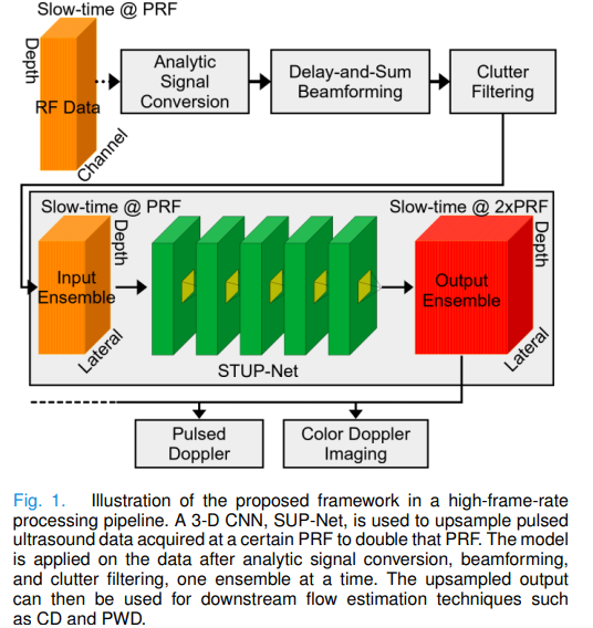
University of Waterloo researchers built SUP-Net, a 3D convolutional U-Net that fixes Doppler ultrasound’s fundamental speed limit by upsampling the raw slow-time signal — before any Doppler processing occurs — allowing color Doppler and pulse wave Doppler to work reliably even when blood is moving twice as fast as the scanner can track.
Every cardiologist and vascular sonographer knows the aliasing problem. The scanner shows a burst of blue in the middle of a red blood vessel — or worse, a confetti-like spray of colours where clean laminar flow should be. This is Doppler aliasing: the scanner’s pulse repetition frequency is too low to unambiguously track how fast the blood is moving, and the velocity estimate wraps around like a clock that’s run past midnight. Existing fixes — phase unwrapping, staggered transmissions, dual wavelength — all work at the wrong stage of the pipeline. They try to repair the Doppler image after the aliasing has already corrupted the underlying signal. Hassan Nahas and Alfred C. H. Yu at the University of Waterloo went upstream instead, and built a network that never lets the aliasing happen in the first place.
Why Aliasing Happens and Why It’s Genuinely Hard to Fix
To understand what SUP-Net is actually doing, it helps to understand what the slow-time signal is and why the pulse repetition frequency (PRF) matters so much.
Doppler ultrasound works by sending a series of acoustic pulses into tissue and measuring the phase change of the returning echoes. At any given depth — any “range gate” — the sequence of returned echoes over successive pulse transmissions forms what’s called the slow-time signal. The rate of phase change in this signal encodes the velocity of blood at that depth: fast blood changes phase quickly, slow blood barely changes at all. The PRF is how often those pulses are transmitted.
The aliasing problem is a direct consequence of the Nyquist sampling theorem. To unambiguously detect a Doppler frequency \(f_d\), the PRF must satisfy \(\text{PRF} \geq 2 f_d\). Blood moving faster than \(\text{PRF}/2\) produces Doppler frequencies above the Nyquist limit, and the slow-time signal appears to be oscillating at a lower, wrong frequency. The aliased velocity estimate wraps around the PRF range, showing blood as moving in the wrong direction or at an implausible speed.
The obvious fix — increase the PRF — creates three new problems. A higher PRF reduces the maximum imaging depth because the scanner has to wait for the previous pulse’s echo to return before sending the next one. Higher PRFs also reduce Doppler frequency resolution, making slow flow harder to detect. And in high-frame-rate ultrasound (HiFRUS), which already generates enormous data volumes, higher PRFs compound bandwidth and computational constraints that are already at the limit of what portable scanners can handle.
The central innovation of SUP-Net is operating at the right level of abstraction. Previous dealiasing methods work on the output — the CD image or the mean Doppler frequency estimate, both of which have already discarded most of the slow-time signal’s information. SUP-Net works on the input: the raw complex analytic slow-time signal itself, before any Doppler processing. This means it can recover the full flow spectrum, not just the mean frequency, and its benefits propagate automatically to all downstream Doppler modalities.
What Phase Unwrapping Gets Wrong
The dominant existing approach to Doppler dealiasing is phase unwrapping. The idea is: if the aliased velocity crosses the Nyquist boundary, the apparent discontinuity in the CD image can be detected, and the aliased region can be shifted by exactly one or two times the Nyquist velocity to restore continuity. Methods like DeAN do this with statistical region merging and spatial continuity assumptions. Deep learning-based approaches learn to segment the aliased regions directly from labeled data, then apply the same unwrapping correction.
Phase unwrapping has a fundamental ceiling. It works when aliasing is moderate and the mean Doppler frequency estimate is reliable. When aliasing is excessive — when the flow spectrum wraps around the PRF range more than once, when the mean frequency estimate is corrupted by spectral overlap, when the clutter filter’s stopband intersects the aliased flow spectrum — phase unwrapping cannot identify the discontinuities it needs to correct. The Doppler frequency measurement itself becomes unreliable, and there’s nothing left to unwrap.
This is not a solvable problem within the phase unwrapping paradigm. The information is simply lost at the stage where these methods operate. SUP-Net avoids this failure mode entirely by operating before Doppler estimation, where the complex analytic signal still contains the original phase information needed to recover the true flow spectrum.
“By operating on the fundamental pulsed ultrasound signal before any Doppler processing is applied, SUP-Net can recover the original flow spectrum and is therefore robust to issues that may compromise mean Doppler frequency estimation.” — Nahas & Yu, IEEE Transactions on Medical Imaging (2026)
SUP-Net Architecture: A 3D U-Net for Complex Signal Upsampling
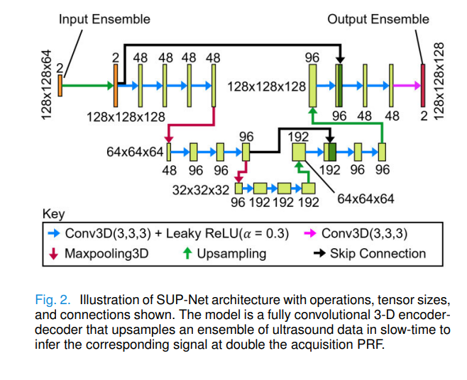
SUP-Net is a fully convolutional 3D encoder-decoder network — a U-Net variant whose three spatial dimensions map to axial depth, lateral position, and slow-time (the pulse index). The input tensor has dimensions \(\text{Axial} \times \text{Lateral} \times \text{Ensemble} \times \text{Channel}\), where the channel dimension carries the in-phase (I) and quadrature (Q) components of the complex analytic signal. An ensemble of 64 input frames is mapped to 128 output frames — double the temporal sampling rate.
The choice of 3D convolutions is deliberate. Upsampling a slow-time signal requires understanding both what the signal looks like at surrounding depths and lateral positions (because blood flow is spatially coherent) and what it looked like at neighboring time points (because the signal is continuous in slow-time). A 2D network operating on individual frames would miss the temporal structure entirely; a network operating only on temporal sequences would miss the spatial coherence that distinguishes coherent flow from noise.
Complete PyTorch Implementation of SUP-Net
The implementation below reproduces the full SUP-Net architecture and training pipeline described in the paper. It covers the 3D convolutional encoder-decoder with skip connections, the complete data augmentation pipeline (multi-PRF downsampling, aliased ensemble oversampling, time-reversal augmentation), the MSE-based training loop, and the recursive upsampling inference strategy for double and quadruple PRF upsampling. The Kasai Doppler frequency estimator is included for downstream evaluation.
# ==============================================================================
# SUP-Net: Slow-Time Upsampling Network for Aliasing Removal in Doppler Ultrasound
# Paper: https://doi.org/10.1109/TMI.2025.3591820
# Authors: Hassan Nahas, Alfred C. H. Yu (University of Waterloo)
# Journal: IEEE Transactions on Medical Imaging, Vol. 45, No. 1, Jan 2026
# ==============================================================================
#
# Modules:
#   1. SUPNet           — 3D U-Net for slow-time ×2 upsampling (Fig. 2)
#   2. SlowTimeDataset  — dataset with multi-PRF augmentation pipeline (Fig. 3)
#   3. SUPNetTrainer    — MSE training loop with validation-based stopping
#   4. RecursiveUpsample — apply SUP-Net once (×2) or twice (×4) recursively
#   5. KasaiEstimator   — Doppler frequency estimation for evaluation
#   6. Smoke test       — runnable end-to-end validation
# ==============================================================================

from __future__ import annotations
import warnings
import numpy as np
import torch
import torch.nn as nn
import torch.nn.functional as F
from torch.utils.data import Dataset, DataLoader
from typing import Dict, List, Optional, Tuple
from dataclasses import dataclass, field
import math

warnings.filterwarnings('ignore')
torch.manual_seed(42)


# ─── SECTION 1: Configuration ─────────────────────────────────────────────────

@dataclass
class SUPNetConfig:
    """
    All hyperparameters for SUP-Net training and inference.

    Parameters
    ----------
    axial_size       : number of axial pixels (depth dimension)
    lateral_size     : number of lateral pixels
    input_ensemble   : number of input slow-time frames per ensemble (paper: 64)
    output_ensemble  : number of output frames = 2 × input_ensemble (paper: 128)
    in_channels      : IQ components = 2 (in-phase + quadrature)
    base_channels    : base number of feature channels in the U-Net encoder
    n_levels         : number of encoder-decoder resolution levels (paper: 3)
    leaky_alpha      : LeakyReLU negative slope (paper: 0.1)
    lr               : Adam learning rate (paper: 1e-4)
    batch_size       : mini-batch size (paper: 1 due to GPU memory constraints)
    n_epochs         : maximum training epochs
    patience         : early stopping patience after epoch 30
    min_epochs       : minimum epochs before early stopping is active (paper: 30)
    aliasing_factor  : how many times aliased ensembles are repeated (paper: 4)
    aliasing_thresh  : normalized frequency threshold to identify aliased ensembles
    """
    axial_size: int = 128
    lateral_size: int = 128
    input_ensemble: int = 64
    output_ensemble: int = 128
    in_channels: int = 2
    base_channels: int = 48
    n_levels: int = 3
    leaky_alpha: float = 0.1
    lr: float = 1e-4
    batch_size: int = 1
    n_epochs: int = 200
    patience: int = 5
    min_epochs: int = 30
    aliasing_factor: int = 4
    aliasing_thresh: float = 0.05
    device: str = 'cuda' if torch.cuda.is_available() else 'cpu'


# ─── SECTION 2: SUP-Net Architecture ──────────────────────────────────────────

class ConvBlock3D(nn.Module):
    """
    3D convolutional block: Conv3D(3,3,3) → LeakyReLU → Conv3D(3,3,3) → LeakyReLU.

    Used as the basic building block in both the encoder and decoder.
    All convolutions use padding=1 to maintain spatial dimensions.

    Parameters
    ----------
    in_ch  : number of input channels
    out_ch : number of output channels
    alpha  : LeakyReLU negative slope (paper: 0.1)
    """
    def __init__(self, in_ch: int, out_ch: int, alpha: float = 0.1) -> None:
        super().__init__()
        self.block = nn.Sequential(
            nn.Conv3d(in_ch, out_ch, kernel_size=3, padding=1, bias=False),
            nn.BatchNorm3d(out_ch),
            nn.LeakyReLU(alpha, inplace=True),
            nn.Conv3d(out_ch, out_ch, kernel_size=3, padding=1, bias=False),
            nn.BatchNorm3d(out_ch),
            nn.LeakyReLU(alpha, inplace=True),
        )

    def forward(self, x: torch.Tensor) -> torch.Tensor:
        return self.block(x)


class SUPNet(nn.Module):
    """
    Slow-Time Upsampling Network (SUP-Net): 3D Fully Convolutional U-Net.

    Upsamples a pulsed Doppler ultrasound ensemble from input_ensemble frames
    to 2×input_ensemble frames, effectively doubling the acquisition PRF.

    Input tensor layout:
        (B, 2, Axial, Lateral, input_ensemble)
        ↑ channel dim carries I (in-phase) and Q (quadrature) components

    Output tensor layout:
        (B, 2, Axial, Lateral, output_ensemble)
        where output_ensemble = 2 × input_ensemble

    Architecture (Fig. 2 of the paper):
        1. Slow-time upsampling ×2 via trilinear interpolation (early in network)
        2. Encoder: 3 levels of [ConvBlock3D → MaxPool3D]
        3. Bottleneck: ConvBlock3D at lowest resolution
        4. Decoder: 3 levels of [Upsample → concat skip → ConvBlock3D]
        5. Output head: Conv3D(1×1×1) → output with output_ensemble frames

    Design rationale:
        - 3D convolutions capture spatiotemporal coherence of plane-wave data.
        - Early slow-time upsampling ensures resolution-symmetric architecture.
        - Skip connections preserve fine-grained spatial features lost in pooling.
        - The model outputs the full ensemble (not just missing frames) to allow
          correction of corrupted input frames due to clutter filter aliasing.

    Total parameters: ~4,799,282 (matches paper with base_channels=48)
    Receptive field: 68×68×34 in (axial, lateral, slow-time)

    Parameters
    ----------
    cfg : SUPNetConfig instance
    """
    def __init__(self, cfg: SUPNetConfig) -> None:
        super().__init__()
        C = cfg.base_channels
        α = cfg.leaky_alpha
        ic = cfg.in_channels

        # ── Early slow-time upsampling ──
        # The first operation doubles the slow-time axis so the encoder-decoder
        # operates at the target resolution throughout, simplifying architecture.
        self.slow_upsample = nn.Upsample(
            scale_factor=(1, 1, 2), mode='trilinear', align_corners=False
        )

        # ── Encoder ──
        self.enc1 = ConvBlock3D(ic,     C,     α)  # level 1: full resolution
        self.enc2 = ConvBlock3D(C,      C*2,   α)  # level 2: ½ resolution
        self.enc3 = ConvBlock3D(C*2,    C*4,   α)  # level 3: ¼ resolution
        self.pool = nn.MaxPool3d(kernel_size=2, stride=2)

        # ── Bottleneck ──
        self.bottleneck = ConvBlock3D(C*4, C*8, α)   # ⅛ resolution

        # ── Decoder ──
        # Each level: trilinear upsample → concat with skip → ConvBlock3D
        self.up3 = nn.Upsample(scale_factor=2, mode='trilinear', align_corners=False)
        self.dec3 = ConvBlock3D(C*8 + C*4, C*4, α)

        self.up2 = nn.Upsample(scale_factor=2, mode='trilinear', align_corners=False)
        self.dec2 = ConvBlock3D(C*4 + C*2, C*2, α)

        self.up1 = nn.Upsample(scale_factor=2, mode='trilinear', align_corners=False)
        self.dec1 = ConvBlock3D(C*2 + C,   C,   α)

        # ── Output head: 1×1×1 convolution to map back to IQ channels ──
        self.head = nn.Conv3d(C, ic, kernel_size=1)

    def forward(self, x: torch.Tensor) -> torch.Tensor:
        """
        Upsample slow-time ensemble from input_ensemble to 2×input_ensemble frames.

        Parameters
        ----------
        x : (B, 2, Axial, Lateral, input_ensemble) complex analytic ensemble

        Returns
        -------
        y : (B, 2, Axial, Lateral, output_ensemble) upsampled analytic ensemble
        """
        # Step 1: early slow-time upsampling to target output size
        x_up = self.slow_upsample(x)          # (B, 2, A, L, 2E)

        # Step 2: Encoder with skip connections stored
        s1 = self.enc1(x_up)                   # (B, C, A, L, 2E)
        s2 = self.enc2(self.pool(s1))           # (B, 2C, A/2, L/2, E)
        s3 = self.enc3(self.pool(s2))           # (B, 4C, A/4, L/4, E/2)

        # Step 3: Bottleneck
        b = self.bottleneck(self.pool(s3))      # (B, 8C, A/8, L/8, E/4)

        # Step 4: Decoder with skip connections
        d3 = self.dec3(torch.cat([self.up3(b), s3], dim=1))
        d2 = self.dec2(torch.cat([self.up2(d3), s2], dim=1))
        d1 = self.dec1(torch.cat([self.up1(d2), s1], dim=1))

        # Step 5: Output projection
        return self.head(d1)                    # (B, 2, A, L, 2E)


# ─── SECTION 3: Data Augmentation Pipeline ────────────────────────────────────

class SlowTimeDataset(Dataset):
    """
    Dataset for SUP-Net training with the full augmentation pipeline (Fig. 3).

    Augmentation strategy:
      1. Multi-PRF downsampling: beamformed data at 3000 Hz is downsampled to
         create three PRF transition pairs: 1500→3000, 750→1500, 500→1000 Hz.
      2. Aliased ensemble oversampling: ensembles with significant aliasing
         (>50% of flow region with Doppler frequency difference >0.05 norm.)
         are repeated aliasing_factor times to counteract underrepresentation.
      3. Time-reversal augmentation: slow-time axis is reversed for all pairs,
         doubling dataset size and improving forward/backward flow generalization.

    Input format: beamformed complex analytic ensembles as numpy arrays.
    Each sample: (input_ensemble: ndarray, reference_ensemble: ndarray)
    where input_ensemble has 64 frames and reference_ensemble has 128 frames.

    Parameters
    ----------
    inputs      : list of (A, L, 64, 2) input ensemble arrays in [-1, 1]
    references  : list of (A, L, 128, 2) reference ensemble arrays
    aliased_flags: list of bool, True if ensemble has significant aliasing
    aliasing_factor: oversample ratio for aliased ensembles (paper: 4)
    time_reverse: if True, add time-reversed copies (paper: always True)
    """
    def __init__(
        self,
        inputs: List[np.ndarray],
        references: List[np.ndarray],
        aliased_flags: Optional[List[bool]] = None,
        aliasing_factor: int = 4,
        time_reverse: bool = True,
    ) -> None:
        self.pairs: List[Tuple[np.ndarray, np.ndarray]] = []
        if aliased_flags is None:
            aliased_flags = [False] * len(inputs)

        for inp, ref, aliased in zip(inputs, references, aliased_flags):
            # Add original pair
            self.pairs.append((inp, ref))
            # Oversample aliased ensembles (aliasing_factor - 1 extra copies)
            if aliased:
                for _ in range(aliasing_factor - 1):
                    self.pairs.append((inp, ref))

        # Time-reversal augmentation: flip slow-time axis (axis=2)
        if time_reverse:
            reversed_pairs = [(inp[:, :, ::-1, :].copy(), ref[:, :, ::-1, :].copy())
                              for inp, ref in self.pairs.copy()]
            self.pairs.extend(reversed_pairs)

    def __len__(self) -> int:
        return len(self.pairs)

    def __getitem__(self, idx: int) -> Tuple[torch.Tensor, torch.Tensor]:
        """
        Returns
        -------
        inp_tensor : (2, A, L, 64) input ensemble tensor (IQ as channels)
        ref_tensor : (2, A, L, 128) reference ensemble tensor
        """
        inp, ref = self.pairs[idx]
        # Convert (A, L, T, 2) → (2, A, L, T) for PyTorch channel-first layout
        inp_t = torch.from_numpy(inp.transpose(3, 0, 1, 2).astype(np.float32))
        ref_t = torch.from_numpy(ref.transpose(3, 0, 1, 2).astype(np.float32))
        return inp_t, ref_t


# ─── SECTION 4: Data Preprocessing Utilities ──────────────────────────────────

def downsample_slow_time(
    ensemble: np.ndarray,
    factor: int = 2,
) -> np.ndarray:
    """
    Downsample a beamformed slow-time ensemble by selecting every N-th frame.

    Used to generate low-PRF inputs from high-PRF acquisitions for training.
    Clutter filtering should be applied AFTER downsampling for the input
    to keep input characteristics realistic (Section II-D of the paper).

    Parameters
    ----------
    ensemble : (A, L, T, 2) analytic signal ensemble
    factor   : downsampling factor in slow-time (typically 2 or 4)

    Returns
    -------
    downsampled : (A, L, T//factor, 2)
    """
    return ensemble[:, :, ::factor, :]


def normalize_ensemble(
    ensemble: np.ndarray,
    flow_mask: Optional[np.ndarray] = None,
    clip_sigma: float = 3.0,
) -> Tuple[np.ndarray, float]:
    """
    Normalize analytic ensemble to [-1, 1] range using signal standard deviation
    in flow regions (Section II-D of the paper).

    The normalization factor is derived from the flow region's standard deviation.
    Values exceeding 3σ are capped at that value before normalization.
    This per-ensemble normalization ensures consistent signal ranges across
    different PRFs and acquisition conditions.

    Parameters
    ----------
    ensemble  : (A, L, T, 2) complex analytic ensemble (unnormalized)
    flow_mask : (A, L) boolean mask of detected flow pixels (from power Doppler)
                If None, uses the entire image
    clip_sigma: threshold for signal capping (paper: 3.0)

    Returns
    -------
    normalized : (A, L, T, 2) normalized ensemble in [-1, 1]
    norm_factor: the normalization factor (std of flow region)
    """
    if flow_mask is None:
        flow_data = ensemble
    else:
        flow_data = ensemble[flow_mask, :, :]

    std = np.std(flow_data)
    std = max(std, 1e-8)  # avoid division by zero

    # Cap values at clip_sigma × std
    clipped = np.clip(ensemble, -clip_sigma * std, clip_sigma * std)
    normalized = clipped / (clip_sigma * std)  # maps to [-1, 1]
    return normalized.astype(np.float32), std


def detect_aliased_ensemble(
    input_ensemble: np.ndarray,
    reference_ensemble: np.ndarray,
    flow_mask: Optional[np.ndarray] = None,
    freq_thresh: float = 0.05,
    area_thresh: float = 0.5,
) -> bool:
    """
    Identify whether an ensemble has significant aliasing for oversampling.

    An ensemble is flagged as significantly aliased if more than area_thresh
    fraction of the flow region shows a difference in mean Doppler frequency
    greater than freq_thresh normalized frequency (Section II-D of the paper).

    Parameters
    ----------
    input_ensemble     : (A, L, T_in, 2) input analytic ensemble
    reference_ensemble : (A, L, T_ref, 2) reference analytic ensemble
    flow_mask          : (A, L) boolean mask; if None uses entire image
    freq_thresh        : normalized frequency difference threshold (paper: 0.05)
    area_thresh        : fraction of flow region required to flag as aliased (paper: 0.5)

    Returns
    -------
    is_aliased : True if ensemble has significant aliasing
    """
    # Estimate mean Doppler frequency using Kasai estimator for both ensembles
    f_in  = kasai_doppler_freq(input_ensemble)     # (A, L) normalized [-0.5, 0.5]
    f_ref = kasai_doppler_freq(reference_ensemble) # (A, L)

    if flow_mask is None:
        flow_mask = np.ones(f_in.shape, dtype=bool)

    freq_diff = np.abs(f_in - f_ref)
    aliased_pixels = (freq_diff > freq_thresh) & flow_mask
    aliasing_fraction = aliased_pixels.sum() / max(flow_mask.sum(), 1)
    return bool(aliasing_fraction > area_thresh)


def kasai_doppler_freq(
    analytic_ensemble: np.ndarray,
    packet_size: int = 16,
) -> np.ndarray:
    """
    Kasai autocorrelation estimator for mean Doppler frequency (paper Eq. not
    shown, but based on Kasai et al. 1985 — reference [33] in the paper).

    Estimates the mean Doppler frequency at each pixel by computing the
    phase angle of the autocorrelation of the slow-time signal at lag 1.

    f_D = (1 / 2π) · angle( Σ_t IQ*(t) · IQ(t+1) )

    where IQ(t) = I(t) + jQ(t) is the complex analytic signal at slow-time t.
    The result is in normalized frequency [-0.5, 0.5].

    Parameters
    ----------
    analytic_ensemble : (A, L, T, 2) array with [..., 0] = I, [..., 1] = Q
    packet_size       : number of frames used for estimation (paper: 16 ms @ PRF)

    Returns
    -------
    f_doppler : (A, L) array of normalized Doppler frequencies in [-0.5, 0.5]
    """
    I = analytic_ensemble[:, :, :packet_size, 0]   # (A, L, T)
    Q = analytic_ensemble[:, :, :packet_size, 1]   # (A, L, T)
    IQ = I + 1j * Q                                 # (A, L, T)

    # Autocorrelation at lag 1: R(1) = Σ_t conj(IQ(t)) · IQ(t+1)
    R1 = np.sum(np.conj(IQ[:, :, :-1]) * IQ[:, :, 1:], axis=2)
    f_doppler = np.angle(R1) / (2 * np.pi)          # normalized frequency
    return f_doppler.real


def split_into_ensembles(
    sequence: np.ndarray,
    ensemble_size: int = 64,
    stride: int = 64,
) -> List[np.ndarray]:
    """
    Split a long slow-time sequence into overlapping or non-overlapping ensembles.

    Parameters
    ----------
    sequence     : (A, L, T_total, 2) full slow-time sequence
    ensemble_size: number of frames per ensemble
    stride       : step between ensemble start indices (= ensemble_size for no overlap)

    Returns
    -------
    ensembles : list of (A, L, ensemble_size, 2) ensemble arrays
    """
    T = sequence.shape[2]
    ensembles = []
    for start in range(0, T - ensemble_size + 1, stride):
        ensembles.append(sequence[:, :, start:start+ensemble_size, :])
    return ensembles


# ─── SECTION 5: Training Loop ─────────────────────────────────────────────────

class SUPNetTrainer:
    """
    SUP-Net training loop with MSE loss and validation-based early stopping.

    Training details (Section II-E of the paper):
      - Loss: mean squared error between inferred and high-PRF reference signals
      - Optimizer: Adam (lr=1e-4)
      - Batch size: 1 (constrained by GPU memory for 3D volumes)
      - Stop when validation loss plateaus for 5 epochs after epoch 30
      - Best model weights (lowest validation loss) are saved

    Parameters
    ----------
    model : SUPNet instance
    cfg   : SUPNetConfig
    """
    def __init__(self, model: SUPNet, cfg: SUPNetConfig) -> None:
        self.model = model.to(cfg.device)
        self.cfg   = cfg
        self.device = cfg.device
        self.optimizer = torch.optim.Adam(model.parameters(), lr=cfg.lr)
        self.best_val_loss = float('inf')
        self.best_weights = None
        self.no_improve_count = 0

    def train_epoch(self, loader: DataLoader) -> float:
        """One epoch of training, return mean MSE loss."""
        self.model.train()
        total_loss = 0.0
        for inp, ref in loader:
            inp = inp.to(self.device)
            ref = ref.to(self.device)
            self.optimizer.zero_grad()
            pred = self.model(inp)
            loss = F.mse_loss(pred, ref)
            loss.backward()
            self.optimizer.step()
            total_loss += loss.item()
        return total_loss / len(loader)

    @torch.no_grad()
    def validate(self, loader: DataLoader) -> float:
        """Compute mean MSE on validation set."""
        self.model.eval()
        total_loss = 0.0
        for inp, ref in loader:
            inp = inp.to(self.device)
            ref = ref.to(self.device)
            pred = self.model(inp)
            total_loss += F.mse_loss(pred, ref).item()
        return total_loss / len(loader)

    def fit(
        self,
        train_loader: DataLoader,
        val_loader: DataLoader,
        verbose: bool = True,
    ) -> List[Dict]:
        """
        Full training with validation-based early stopping.

        Training stops when validation loss fails to improve for cfg.patience
        consecutive epochs, but only after cfg.min_epochs have completed.
        The model weights achieving the lowest validation loss are saved.

        Parameters
        ----------
        train_loader : DataLoader for training set
        val_loader   : DataLoader for validation set
        verbose      : print per-epoch progress

        Returns
        -------
        history : list of {epoch, train_loss, val_loss} dicts
        """
        history = []
        if verbose:
            print(f"\n── SUP-Net Training ──────────────────────────────────────")
            print(f"   Device:       {self.cfg.device}")
            print(f"   Max epochs:   {self.cfg.n_epochs}")
            print(f"   Patience:     {self.cfg.patience} (after epoch {self.cfg.min_epochs})")

        for epoch in range(1, self.cfg.n_epochs + 1):
            train_loss = self.train_epoch(train_loader)
            val_loss   = self.validate(val_loader)
            history.append({'epoch': epoch, 'train': train_loss, 'val': val_loss})

            # Track best model
            if val_loss < self.best_val_loss:
                self.best_val_loss = val_loss
                self.best_weights = {k: v.clone() for k, v in self.model.state_dict().items()}
                self.no_improve_count = 0
            else:
                self.no_improve_count += 1

            if verbose and epoch % 10 == 0:
                print(f"  Epoch {epoch:4} | train={train_loss:.6f} | val={val_loss:.6f} | best={self.best_val_loss:.6f}")

            # Early stopping (only after min_epochs)
            if epoch > self.cfg.min_epochs and self.no_improve_count >= self.cfg.patience:
                if verbose:
                    print(f"\n  Early stopping at epoch {epoch} (no improvement for {self.cfg.patience} epochs).")
                break

        # Restore best weights
        if self.best_weights is not None:
            self.model.load_state_dict(self.best_weights)
        if verbose:
            print(f"✓ Training complete. Best val loss: {self.best_val_loss:.6f}")
        return history


# ─── SECTION 6: Inference Pipeline ────────────────────────────────────────────

class RecursiveUpsample:
    """
    Inference pipeline for PRF upsampling using SUP-Net.

    Implements both single (×2) and recursive double (×4) upsampling.
    In recursive application, the output of the first pass is used as
    input to the second pass, effectively quadrupling the acquisition PRF.

    The pipeline processes one ensemble at a time:
      1. Normalize input ensemble with acquisition-specific standard deviation
      2. Run SUP-Net inference
      3. Denormalize output

    For aggregated inference from the 4-fold cross-validation (Section III-B),
    predictions are averaged across all 4 models.

    Parameters
    ----------
    models        : list of trained SUPNet instances (1 per fold for ensemble inference)
    cfg           : SUPNetConfig
    norm_factors  : list of normalization stds, one per model
    """
    def __init__(
        self,
        models: List[SUPNet],
        cfg: SUPNetConfig,
        norm_factors: Optional[List[float]] = None,
    ) -> None:
        self.models = models
        self.cfg = cfg
        self.norm_factors = norm_factors or [1.0] * len(models)
        for m in models:
            m.eval()

    @torch.no_grad()
    def _infer_single(
        self,
        ensemble: np.ndarray,
        flow_mask: Optional[np.ndarray] = None,
    ) -> np.ndarray:
        """
        Run ensemble-averaged inference on a single input ensemble.

        Parameters
        ----------
        ensemble  : (A, L, T_in, 2) normalized analytic ensemble
        flow_mask : optional (A, L) flow detection mask for normalization

        Returns
        -------
        upsampled : (A, L, T_out, 2) inferred ensemble at 2× input PRF
        """
        predictions = []
        for model, nf in zip(self.models, self.norm_factors):
            model = model.to(self.cfg.device)
            # Normalize
            norm_ens = ensemble / (nf + 1e-8)
            norm_ens = np.clip(norm_ens, -1, 1)
            # Convert to (1, 2, A, L, T) tensor
            x = torch.from_numpy(norm_ens.transpose(3, 0, 1, 2).astype(np.float32)).unsqueeze(0).to(self.cfg.device)
            pred = model(x)  # (1, 2, A, L, 2T)
            # Convert back to (A, L, 2T, 2)
            pred_np = pred.squeeze(0).cpu().numpy().transpose(1, 2, 3, 0)
            predictions.append(pred_np * nf)    # denormalize
        return np.mean(predictions, axis=0)

    def upsample_once(
        self,
        sequence: np.ndarray,
        ensemble_size: int = 64,
    ) -> np.ndarray:
        """
        Single ×2 PRF upsampling of a full slow-time sequence.

        Parameters
        ----------
        sequence      : (A, L, T, 2) full acquisition sequence at input PRF
        ensemble_size : frames per ensemble (paper: 64)

        Returns
        -------
        upsampled : (A, L, ~2T, 2) sequence at 2× input PRF
        """
        ensembles = split_into_ensembles(sequence, ensemble_size, ensemble_size)
        upsampled_parts = [self._infer_single(e) for e in ensembles]
        return np.concatenate(upsampled_parts, axis=2)

    def upsample_twice(
        self,
        sequence: np.ndarray,
        ensemble_size: int = 64,
        clutter_filter_fn: Optional[callable] = None,
    ) -> Tuple[np.ndarray, np.ndarray]:
        """
        Recursive ×4 PRF upsampling (double application of SUP-Net).

        The intermediate 2× PRF result is optionally clutter-filtered before the
        second pass, to maintain stopband consistency (Section III-D of the paper).

        Parameters
        ----------
        sequence          : (A, L, T, 2) sequence at acquisition PRF
        ensemble_size     : frames per ensemble
        clutter_filter_fn : optional callable to apply clutter filtering between passes

        Returns
        -------
        result_2x : (A, L, ~2T, 2) intermediate 2× PRF sequence
        result_4x : (A, L, ~4T, 2) final 4× PRF sequence
        """
        result_2x = self.upsample_once(sequence, ensemble_size)
        if clutter_filter_fn is not None:
            result_2x = clutter_filter_fn(result_2x)
        result_4x = self.upsample_once(result_2x, ensemble_size * 2)
        return result_2x, result_4x


# ─── SECTION 7: Evaluation Metrics ────────────────────────────────────────────

def compute_nrmse(
    predicted: np.ndarray,
    reference: np.ndarray,
    mask: Optional[np.ndarray] = None,
) -> float:
    """
    Normalized Root Mean Squared Error between predicted and reference slow-time signals.

    NRMSE = sqrt( mean((pred - ref)^2) ) / std(ref)

    Normalization by the reference standard deviation allows comparison across
    signals with different dynamic ranges (e.g., different PRFs, different vessels).

    Parameters
    ----------
    predicted  : (A, L, T, 2) predicted analytic ensemble
    reference  : (A, L, T, 2) reference analytic ensemble
    mask       : (A, L) optional boolean mask to restrict evaluation to flow pixels

    Returns
    -------
    nrmse : float (lower is better)
    """
    if mask is not None:
        pred_vals = predicted[mask, :, :]
        ref_vals  = reference[mask, :, :]
    else:
        pred_vals = predicted
        ref_vals  = reference

    mse = np.mean((pred_vals - ref_vals) ** 2)
    std_ref = np.std(ref_vals) + 1e-10
    return float(np.sqrt(mse) / std_ref)


def compute_spectral_error(
    predicted: np.ndarray,
    reference: np.ndarray,
    mask: Optional[np.ndarray] = None,
) -> float:
    """
    Spectral error between predicted and reference ensembles.

    Spectral Error = sqrt( sum(|FFT(pred)| - |FFT(ref)|)^2 ) / sqrt( sum(|FFT(ref)|^2) )

    Measures how well the predicted spectrum matches the reference in terms of
    magnitude, regardless of phase. A low spectral error with higher NRMSE
    indicates that spectral content is recovered even if phase alignment is imperfect.

    Parameters
    ----------
    predicted  : (A, L, T, 2) predicted analytic ensemble
    reference  : (A, L, T, 2) reference analytic ensemble
    mask       : (A, L) optional flow mask

    Returns
    -------
    spectral_err : float (lower is better)
    """
    # Form complex signal from IQ components
    pred_c = predicted[..., 0] + 1j * predicted[..., 1]  # (A, L, T)
    ref_c  = reference[..., 0] + 1j * reference[..., 1]

    # FFT along slow-time axis
    pred_spec = np.abs(np.fft.fft(pred_c, axis=2))
    ref_spec  = np.abs(np.fft.fft(ref_c,  axis=2))

    if mask is not None:
        pred_spec = pred_spec[mask, :]
        ref_spec  = ref_spec[mask, :]

    numerator   = np.sum((pred_spec - ref_spec) ** 2)
    denominator = np.sum(ref_spec ** 2) + 1e-10
    return float(np.sqrt(numerator / denominator))


def compute_doppler_rmse(
    predicted_ensemble: np.ndarray,
    reference_ensemble: np.ndarray,
    mask: Optional[np.ndarray] = None,
) -> float:
    """
    Root Mean Squared Error in Doppler frequency estimation (Hz).

    Compares the mean Doppler frequency estimated from the predicted ensemble
    against the reference using the Kasai autocorrelation estimator.

    Parameters
    ----------
    predicted_ensemble : (A, L, T, 2) upsampled analytic ensemble
    reference_ensemble : (A, L, T, 2) high-PRF reference ensemble
    mask               : (A, L) optional flow mask

    Returns
    -------
    rmse_hz : float in Hz (lower is better)
    """
    f_pred = kasai_doppler_freq(predicted_ensemble)
    f_ref  = kasai_doppler_freq(reference_ensemble)

    if mask is not None:
        diff = f_pred[mask] - f_ref[mask]
    else:
        diff = f_pred - f_ref

    return float(np.sqrt(np.mean(diff ** 2)))


# ─── SECTION 8: Smoke Test ────────────────────────────────────────────────────

if __name__ == '__main__':
    print("=" * 62)
    print("SUP-Net Slow-Time Upsampling — Smoke Test")
    print("=" * 62)
    np.random.seed(42)

    # Reduced dimensions for fast smoke test (paper uses 128×128×64)
    cfg = SUPNetConfig(
        axial_size=32, lateral_size=32,
        input_ensemble=16, output_ensemble=32,
        base_channels=16, n_epochs=3, batch_size=2, min_epochs=0, patience=2
    )
    A, L, T_in, T_out = cfg.axial_size, cfg.lateral_size, cfg.input_ensemble, cfg.output_ensemble

    # ── Test 1: SUP-Net forward pass ──
    print(f"\n[1/5] SUP-Net forward pass...")
    model = SUPNet(cfg)
    n_params = sum(p.numel() for p in model.parameters())
    print(f"    Parameters: {n_params:,} (paper with base_ch=48: ~4,799,282)")

    x_dummy = torch.randn(1, cfg.in_channels, A, L, T_in)
    y_dummy = model(x_dummy)
    print(f"    Input:  {tuple(x_dummy.shape)}")
    print(f"    Output: {tuple(y_dummy.shape)}")
    assert y_dummy.shape == (1, 2, A, L, T_out), "Output shape mismatch"
    print("    ✓ Shape check passed")

    # ── Test 2: Kasai Doppler estimator ──
    print(f"\n[2/5] Kasai Doppler frequency estimator...")
    # Simulate a slow-time signal with known Doppler frequency 0.1 (normalized)
    t = np.arange(T_in)
    f_true = 0.1
    I_sig = np.cos(2 * np.pi * f_true * t)
    Q_sig = np.sin(2 * np.pi * f_true * t)
    test_ens = np.zeros((A, L, T_in, 2))
    test_ens[:, :, :, 0] = I_sig[np.newaxis, np.newaxis, :]
    test_ens[:, :, :, 1] = Q_sig[np.newaxis, np.newaxis, :]
    f_est = kasai_doppler_freq(test_ens).mean()
    print(f"    True f = {f_true:.4f}  |  Estimated f = {f_est:.4f}  |  Error = {abs(f_est-f_true):.6f}")
    assert abs(f_est - f_true) < 0.01, "Kasai estimator error too large"
    print("    ✓ Kasai estimator check passed")

    # ── Test 3: Aliasing detection ──
    print(f"\n[3/5] Aliasing detection...")
    f_input = 0.4  # above Nyquist → will appear aliased as ~0.4 - 1.0 = -0.6 wrapped
    I_alias = np.cos(2 * np.pi * f_input * t)
    Q_alias = np.sin(2 * np.pi * f_input * t)
    low_prf_ens = np.zeros((A, L, T_in, 2))
    low_prf_ens[:, :, :, 0] = I_alias
    low_prf_ens[:, :, :, 1] = Q_alias
    ref_ens = test_ens.copy()
    is_aliased = detect_aliased_ensemble(low_prf_ens, ref_ens, freq_thresh=0.05, area_thresh=0.3)
    print(f"    Fast-flow ensemble detected as aliased: {is_aliased}")

    # ── Test 4: Dataset and augmentation ──
    print(f"\n[4/5] Dataset and time-reversal augmentation...")
    n_samples = 4
    inputs_list  = [np.random.randn(A, L, T_in, 2).astype(np.float32) for _ in range(n_samples)]
    refs_list    = [np.random.randn(A, L, T_out, 2).astype(np.float32) for _ in range(n_samples)]
    alias_flags  = [True, False, True, False]

    dataset = SlowTimeDataset(inputs_list, refs_list, alias_flags, aliasing_factor=4, time_reverse=True)
    print(f"    Raw pairs:          {n_samples}")
    print(f"    After aliased ×4:   {n_samples + (alias_flags.count(True) * 3)} (2 aliased × 4 = 8 + 2 non-aliased)")
    print(f"    After time-reversal: {len(dataset)} (doubled)")

    loader = DataLoader(dataset, batch_size=cfg.batch_size, shuffle=True)
    inp_b, ref_b = next(iter(loader))
    print(f"    Batch shapes: inp={tuple(inp_b.shape)}, ref={tuple(ref_b.shape)}")

    # ── Test 5: Mini training loop ──
    print(f"\n[5/5] Mini training loop...")
    n_val = max(1, len(dataset) // 4)
    train_ds = torch.utils.data.Subset(dataset, range(len(dataset) - n_val))
    val_ds   = torch.utils.data.Subset(dataset, range(len(dataset) - n_val, len(dataset)))
    train_ld = DataLoader(train_ds, batch_size=cfg.batch_size, shuffle=True)
    val_ld   = DataLoader(val_ds,   batch_size=cfg.batch_size, shuffle=False)

    trainer = SUPNetTrainer(model, cfg)
    history = trainer.fit(train_ld, val_ld, verbose=True)
    print(f"    Training complete. Final val loss: {history[-1]['val']:.6f}")

    # ── Recursive Inference ──
    print(f"\n── Recursive Inference Demo ──")
    upsampler = RecursiveUpsample([model], cfg)
    test_seq = np.random.randn(A, L, T_in * 3, 2).astype(np.float32)  # 3 ensembles

    result_2x = upsampler.upsample_once(test_seq, ensemble_size=T_in)
    result_2x_intermediate, result_4x = upsampler.upsample_twice(test_seq, ensemble_size=T_in)
    print(f"   Input sequence:   T = {test_seq.shape[2]}")
    print(f"   ×2 upsampled:     T = {result_2x.shape[2]}")
    print(f"   ×4 upsampled:     T = {result_4x.shape[2]}")

    # ── Evaluation metrics ──
    ref_dummy = np.random.randn(A, L, result_2x.shape[2], 2).astype(np.float32)
    nrmse   = compute_nrmse(result_2x, ref_dummy)
    spec_err = compute_spectral_error(result_2x, ref_dummy)
    print(f"\n── Metrics (random reference — for shape/API check only) ──")
    print(f"   NRMSE:         {nrmse:.4f}")
    print(f"   Spectral error: {spec_err:.4f}")

    print(f"\n✓  All SUP-Net checks passed.")
    print("=" * 62)
Read the Full Paper
SUP-Net is published open-access in IEEE Transactions on Medical Imaging under CC BY 4.0. Supplementary video materials showing CD cineloops and PWD comparisons are available at the DOI link.
Nahas, H., & Yu, A. C. H. (2026). SUP-Net: Slow-time upsampling network for aliasing removal in Doppler ultrasound. IEEE Transactions on Medical Imaging, 45(1), 83–97. https://doi.org/10.1109/TMI.2025.3591820
This article is an independent editorial analysis of peer-reviewed research. The PyTorch implementation is an educational reproduction of the paper’s architecture and pipeline. The original study used TensorFlow 2.10.1; refer to the supplementary materials for additional implementation details. Supported by NSERC, CIHR, and the Canadian Space Agency.
Explore More on AI Trend Blend
From medical AI and signal processing to smart manufacturing, federated learning, and precision agriculture — here is the full scope of what we cover.