Why Flat Classifiers Fail Doctors: H²CL Uses Hyperbolic Geometry to Teach AI the Clinical Hierarchy of Disease
A UNSW Sydney team built H²CL — a dual-geometry image-text framework that simultaneously operates in Euclidean and hyperbolic spaces, combining group contrastive learning with a hyperbolic entailment loss, to classify medical images across clinical taxonomies. The result: 7% accuracy gains over Swin Transformer baselines across cervical cytology, skin lesions, and gallbladder disease.
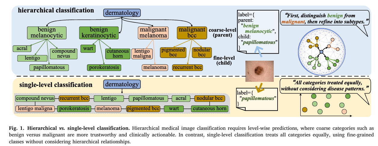
When a dermatologist examines a skin lesion, they don’t jump straight to naming a subtype. They first ask: benign or malignant? If benign, then which broad family — melanocytic or keratinocytic? Only after establishing those coarser categories do they zoom in to the specific subtype. This hierarchical, level-by-level reasoning isn’t just clinical habit — it’s a safety mechanism. Calling something “papillomatous” when you should have called it “malignant melanoma” is catastrophically worse than getting the specific subtype slightly wrong. For years, medical image AI has ignored this logic entirely, flattening every disease into a single list and training classifiers that treat all errors as equal. A team from UNSW Sydney and Monash University decided that enough was enough.
The Problem with Flat Classifiers in a Hierarchical World
Clinical medicine is organized as a tree, not a list. At the top sit broad, actionable categories — benign versus malignant, reactive versus neoplastic. Below them sit increasingly specific subtypes that guide treatment decisions. The branches of this tree are not arbitrary: they reflect actual biological and etiological relationships. Benign melanocytic lesions share molecular characteristics because they share developmental origins, and that shared biology shows up as shared visual features.
A standard softmax classifier sees none of this. It treats “malignant melanoma” and “papillomatous nevus” as two equally distant options, no different from “car” and “airplane.” When it gets confused between adjacent subtypes within the same family, it pays the same penalty as when it confuses a benign lesion with a malignant one. In deployment, those two types of error have vastly different clinical consequences.
There’s another fundamental problem: medical images are visually treacherous. Low-grade and high-grade squamous intraepithelial lesions on a cervical cytology slide can look nearly identical to untrained eyes — the distinguishing signals are subtle patterns in chromatin distribution. Meanwhile, high-grade SIL itself is visually heterogeneous, with individual cases showing radically different morphologies. Inter-class similarity and intra-class heterogeneity are the defining challenges, and a classifier that treats the label space as flat has no principled mechanism for addressing either.
The core argument of this paper is geometric: flat Euclidean classifiers are the wrong mathematical tool for hierarchical label spaces. Euclidean space grows polynomially, so fitting an exponentially branching taxonomy into it requires exponentially more dimensions. Hyperbolic space grows exponentially with radius by construction — it is the natural geometry for tree-structured data. H²CL uses this property by design rather than by accident.
Why Hyperbolic Space Fits Disease Taxonomies
To understand why hyperbolic geometry matters, consider what happens when you embed a tree into ordinary Euclidean space. A binary tree with depth \(d\) has \(2^d – 1\) nodes. In Euclidean space, representing all those nodes with low distortion requires dimensions that grow roughly as \(2^d\) — exponentially. In a 2D hyperbolic space, you can embed the same tree with distortion that decreases as you add depth, because volume in hyperbolic space expands exponentially with radius. The geometry matches the data structure.
The team works with the Poincaré ball model \(\mathbb{D}^n_c = \{\mathbf{x} \in \mathbb{R}^n : c\|\mathbf{x}\|^2 < 1\}\), where \(c\) controls the curvature. The geodesic distance between two points in this ball is:
The key geometric fact is that near the origin of the Poincaré ball, space looks roughly Euclidean — but near the boundary, infinitesimal distances expand dramatically because the conformal factor \(\lambda^c_\mathbf{x} = 2/(1-c\|\mathbf{x}\|^2)\) diverges. This means that points close to the boundary can be arbitrarily far from each other in geodesic distance, even if they look close in the Euclidean sense. General parent classes naturally cluster near the origin, while specific child classes are pushed toward the boundary — exactly the radial ordering that clinical taxonomies require.
To transition between Euclidean features (from standard neural network layers) and hyperbolic space, the paper uses the exponential map at the origin:
And the inverse logarithmic map \(\log^c_\mathbf{x}\) brings features back to the tangent Euclidean space when operations like attention need to happen in a common coordinate system.
The H²CL Architecture: Three Interlocking Mechanisms
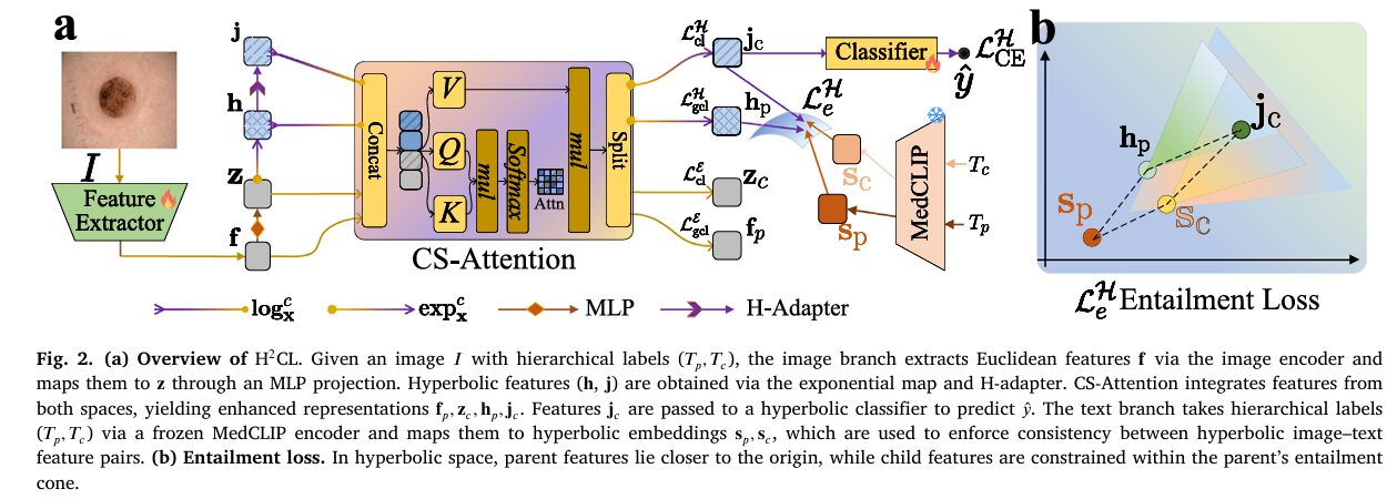
H²CL consists of an image branch and a text branch, designed around three interlocking mechanisms that each address a different aspect of the hierarchical classification problem.
1. Dual-Geometry Feature Extraction with CS-Attention
The image branch starts with any pretrained backbone (the paper primarily uses Swin Transformer) producing Euclidean features \(\mathbf{f} \in \mathbb{R}^m\). An MLP adapter projects \(\mathbf{f}\) to \(\mathbf{z} \in \mathbb{R}^m\). The exponential map then lifts \(\mathbf{z}\) to hyperbolic features \(\mathbf{h} \in \mathbb{D}^m_c\), which are further refined by an H-Adapter (a hyperbolic linear layer) to produce \(\mathbf{j} \in \mathbb{D}^m_c\).
Now the framework has four feature vectors per sample: \(\mathbf{f}, \mathbf{z}\) in Euclidean space and \(\mathbf{h}, \mathbf{j}\) in hyperbolic space. Rather than concatenating them naively, the team introduces Cross-Space Attention (CS-Attention). The hyperbolic features are first mapped to the tangent space via the logarithmic map so everything lives in a common Euclidean coordinate system, then a standard attention operation reweights all four features jointly:
where \(\mathbf{C}_m = [\mathbf{f}, \mathbf{z}, \log^c_\mathbf{x}(\mathbf{h}), \log^c_\mathbf{x}(\mathbf{j})]\) is the concatenation of all four features. The updated hyperbolic features are recovered by applying the exponential map to \(\hat{\mathbf{h}}_p, \hat{\mathbf{j}}_c\). This attention mechanism is the paper’s answer to a genuine challenge: how do you let two fundamentally different geometric spaces talk to each other? The tangent space provides the common ground.
Final prediction uses a hyperbolic Möbius classifier. Each class \(k\) has a learnable prototype \(\mathbf{p}_k\) in the Poincaré ball. The logit for class \(k\) is the negative hyperbolic distance from the transformed feature \(\mathbf{o}\) to the prototype \(\alpha_k = -d_c(\mathbf{o}, \mathbf{p}_k)\), and the hyperbolic cross-entropy loss is:
2. Group Contrastive Learning Across Both Spaces
Standard supervised contrastive learning divides samples into positives (same class) and negatives (different class). H²CL extends this with a richer three-way grouping that exploits the hierarchy. Given a sample \(i\):
- Positives \(\mathcal{P}^c_i\): samples from the same child (fine-grained) class
- Weak positives \(\mathcal{P}^w_i\): samples from the same parent class but a different child class
- Negatives \(\mathcal{N}^c_i\): samples from a different parent class entirely
In Euclidean space, the group CL loss on adapted child-level features \(\mathbf{z}^i_c\) is:
where \(\omega_i = |\mathcal{P}^c_i| / (|\mathcal{P}^c_i| + |\mathcal{P}^w_i|) \in [0,1]\) is a data-driven weight that down-scales the contribution of weak positives. The same structure is applied in hyperbolic space using hyperbolic distances instead of cosine similarity. In Euclidean space, the loss emphasises local morphological differences between adjacent classes. In hyperbolic space, it enforces global taxonomic consistency across the hierarchy.
3. Hyperbolic Entailment Loss from the Text Branch
The text branch takes hierarchical label names — e.g., the parent “benign melanocytic” and the child “papillomatous” — wraps them in domain-specific prompt templates (“A dermatoscopic image of benign melanocytic”), and encodes them with a frozen MedCLIP text encoder. The resulting embeddings are mapped to hyperbolic space via the exponential map: \(\mathbf{s}_p, \mathbf{s}_c \in \mathbb{D}^m_c\).
In hyperbolic space, radial depth correlates with semantic generality. Parent concepts like “benign melanocytic” should sit closer to the origin and span broader angular regions, while child concepts like “papillomatous” should sit farther out in narrower sectors — exactly the geometry of entailment cones. Following MERU, the entailment cone for a feature \(\mathbf{u}\) is defined as \(\psi(\mathbf{u}) = (1 – \|\mathbf{u}\|/\kappa)\) where \(\kappa = 0.1\). Violations are penalised by measuring the exterior angle between features in the tangent space:
This loss enforces that child image features lie within the angular cone of their parent text embedding, and vice versa — simultaneously aligning images with text and enforcing the parent-before-child radial ordering that the taxonomy demands.
The total training objective combines all five loss components:
“By jointly modelling Euclidean and hyperbolic spaces, the proposed method effectively integrates local morphological discrimination with global taxonomic consistency.” — Fan, Sowmya, Meijering, Yu, Ge & Song, Medical Image Analysis (2026)
Three Datasets, Consistent Superiority
The experiments cover HiCervix (39,124 cervical cytology images, 4 parent / 21 child classes), MoleMap (46,698 dermoscopy images, 8 parent / 41 child classes), and UIdataGB (10,792 gallbladder ultrasound images, 4 parent / 9 child classes). Every competing method — from basic backbones to advanced hierarchical classifiers to fine-grained detection methods — is evaluated under identical protocols.
| Method | HiCervix L2 ACC↑ | MoleMap L2 ACC↑ | UIdataGB L2 ACC↑ | HiCervix d-HIE↓ |
|---|---|---|---|---|
| Swin Transformer | 68.3 | 53.2 | 91.1 | 0.301 |
| HCAST (SOTA) | 74.3 | 53.3 | 96.7 | 0.224 |
| HRN | 65.5 | 44.8 | 93.2 | 0.289 |
| MHN | 65.5 | 44.8 | 93.2 | 0.289 |
| H²CL (image-only, ViT) | 73.4 | 55.6 | 97.8 | 0.234 |
| H²CL (full, Swin) | 77.0 | 59.1 | 97.9 | 0.202 |
Table 1: Fine-grained (L2) accuracy and hierarchical distance on three datasets. H²CL outperforms the prior SOTA (HCAST) by 2.7% on HiCervix and 5.8% on MoleMap L2, while achieving a ~10% relative reduction in hierarchical error (d-HIE).
The gains are not cosmetic. On MoleMap at the fine-grained L2 level, H²CL achieves 59.1% accuracy compared to 53.3% for HCAST and 53.2% for vanilla Swin. On HiCervix at L2, it reaches 77.0% while simultaneously reducing the hierarchical distance metric d-HIE to 0.202 — nearly 10% below the previous best. Statistical significance was confirmed with paired t-tests across three seeds: five of six comparisons showed p < 0.05 with Cohen's d consistently exceeding 2.0.
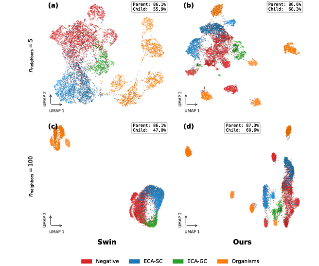
The image-only variant of H²CL (using ViT instead of Swin, without the text branch) already outperforms HCAST on MoleMap and UIdataGB. Adding the text branch addresses the only case where the image-only variant lagged — HiCervix, where text supervision provides the semantic grounding needed to separate the 21 closely related cytology subtypes. This pattern reveals something important: the dual-geometry design alone is powerful, but the entailment-based text alignment is what pushes performance at the most granular levels.
The ablation study tells a clear story. Euclidean-only features achieve 68.3% on HiCervix L2. Hyperbolic-only features improve to 69.9%. Simple concatenation of both reaches 70.5%. CS-Attention fusion jumps to 74.6%. Adding the text branch with standard contrastive loss brings it to 75.8%. Replacing the contrastive loss with the entailment loss achieves 77.0%. Every component earns its keep — and the entailment loss is the biggest single contributor after CS-Attention.
Computational Cost: Nearly Free
H²CL’s most practical selling point may be its overhead profile. For the default Swin Transformer backbone, adding the entire dual-geometry classification head increases parameter count by just 2.6% (195.2M → 200.2M), training time by 0.7%, and inference latency by 0.3%. Memory increases during training because the frozen MedCLIP text encoder must be loaded and the entailment loss computed — but the text branch is discarded entirely at inference time, so test-time memory is essentially unchanged from the baseline. The performance gains come almost for free in deployment.
What Fails and Why
The paper presents failure cases with unusual candor. On HiCervix, the most common errors (MPC→Normal, CC→MPC) suggest that the model sometimes mismatches magnification scale — adjacent cytology categories share morphological features at coarse resolution, and the model lacks multi-scale feature extraction to resolve them at the right level of detail.
On MoleMap, early-stage malignant melanoma is confused with junctional melanocytic lesions because both share asymmetric pigmentation patterns. Basal cell carcinoma is confused with actinic keratosis because limited resolution and specular reflections obscure the keratinization patterns that distinguish them. These are not model failures so much as imaging failures — the discriminating signal simply isn’t present at the resolution captured.
Gallbladder ultrasound confusions arise primarily from co-occurring pathologies. Stones and adenomyomatosis can present simultaneously with inflammatory changes, and the limited spatial resolution of ultrasound makes wall texture analysis unreliable for fine-grained subtype distinction.
In each case, the errors are clinically interpretable — the model fails at the same boundaries that challenge junior clinicians, and the hierarchical structure means that coarse-level decisions remain reliable even when fine-grained prediction is uncertain. That asymmetric reliability is exactly what clinical deployment requires.
Complete PyTorch Implementation
The implementation below faithfully reproduces every component of H²CL described in the paper: the Poincaré ball operations (geodesic distance, exponential map, logarithmic map, Möbius transformation), the CS-Attention cross-geometry fusion module, the group contrastive learning losses in both Euclidean and hyperbolic spaces (Eqs. 3–6), the hyperbolic entailment loss (Eqs. 7–8), the full H²CL model with dual-branch architecture (Eq. 1–2), and the total training objective (Eq. 9). A runnable smoke test with synthetic data closes the file.
# ==============================================================================
# H²CL: Medical Hierarchical Image Classification via Dual-Geometry Image-Text Learning
# Paper: https://doi.org/10.1016/j.media.2026.104120
# Authors: Fan, Sowmya, Meijering, Yu, Ge, Song (UNSW Sydney / Monash University)
# Journal: Medical Image Analysis 112 (2026) 104120
# Code: https://github.com/MCPathology/H2CL
# ==============================================================================
#
# Modules:
# 1. PoincareBall — hyperbolic geometry ops (d_c, exp_c, log_c, Möbius)
# 2. HAdapter — hyperbolic linear layer
# 3. CSAttention — cross-space attention fusion (Eq. 1)
# 4. HyperbolicClassifier — Möbius classifier with prototype logits (Eq. 2)
# 5. GroupCLLoss — Euclidean/hyperbolic group contrastive (Eqs. 3–6)
# 6. EntailmentLoss — hyperbolic entailment + CLIP loss (Eqs. 7–8)
# 7. H2CL — full model with image + text branches (Eq. 9)
# 8. H2CLTrainer — training loop with all losses
# ==============================================================================
from __future__ import annotations
import math, warnings
import numpy as np
import torch
import torch.nn as nn
import torch.nn.functional as F
from torch.utils.data import Dataset, DataLoader
from typing import Dict, List, Optional, Tuple
from dataclasses import dataclass, field
warnings.filterwarnings('ignore')
torch.manual_seed(42)
# ─── SECTION 1: Configuration ─────────────────────────────────────────────────
@dataclass
class H2CLConfig:
"""
All hyperparameters for H²CL.
Parameters
----------
feat_dim : feature dimension m (matches backbone output)
n_parent : number of parent (coarse) classes
n_child : number of child (fine-grained) classes K
curvature : Poincaré ball curvature c (paper: 0.05)
tau : temperature for contrastive losses (paper: 0.5)
kappa : entailment cone boundary constant (paper: 0.1)
lambda_e : weight for Euclidean CL losses
lambda_h : weight for hyperbolic CL losses
lambda_t : weight for entailment loss
lr : learning rate (paper: 1e-5 with Adam)
n_epochs : training epochs (paper: 100)
batch_size : batch size (paper: 32)
n_prompts : number of prompt templates per label (paper: 6)
"""
feat_dim: int = 768
n_parent: int = 4
n_child: int = 21
curvature: float = 0.05
tau: float = 0.5
kappa: float = 0.1
lambda_e: float = 1.0
lambda_h: float = 1.0
lambda_t: float = 1.0
lr: float = 1e-5
n_epochs: int = 100
batch_size: int = 32
n_prompts: int = 6
device: str = 'cuda' if torch.cuda.is_available() else 'cpu'
# ─── SECTION 2: Poincaré Ball Operations ──────────────────────────────────────
class PoincareBall:
"""
Core hyperbolic geometry operations on the Poincaré ball D^n_c.
All methods operate on batched PyTorch tensors and are differentiable.
The base point for exponential/logarithmic maps is fixed at the origin.
Reference: Ganea et al., 2018 (Hyperbolic Neural Networks)
Appendix A of the paper
"""
def __init__(self, curvature: float = 0.05) -> None:
self.c = curvature
def lambda_x(self, x: torch.Tensor) -> torch.Tensor:
"""
Conformal factor λ^c_x = 2 / (1 - c||x||²).
Scales from 2 at the origin to ∞ at the boundary, encoding the
exponential expansion of hyperbolic volume.
Parameters
----------
x : (..., d) point in the Poincaré ball
Returns
-------
lambda_x : (..., 1) conformal factor
"""
x_norm_sq = (x * x).sum(dim=-1, keepdim=True).clamp(max=1 - 1e-5)
return 2 / (1 - self.c * x_norm_sq)
def dist(self, x: torch.Tensor, y: torch.Tensor) -> torch.Tensor:
"""
Geodesic distance d_c(x, y) in the Poincaré ball (Eq. A.1).
d_c(x, y) = (1/√c) · arcosh(1 + 2c||x-y||² / [(1-c||x||²)(1-c||y||²)])
Parameters
----------
x, y : (..., d) points in D^n_c
Returns
-------
dist : (...,) geodesic distances
"""
c = self.c
sqrt_c = math.sqrt(c)
x_norm_sq = (x * x).sum(dim=-1).clamp(max=1 - 1e-5)
y_norm_sq = (y * y).sum(dim=-1).clamp(max=1 - 1e-5)
diff_norm_sq = ((x - y) * (x - y)).sum(dim=-1)
numerator = 2 * c * diff_norm_sq
denominator = (1 - c * x_norm_sq) * (1 - c * y_norm_sq)
arg = 1 + numerator / denominator.clamp(min=1e-6)
return (1 / sqrt_c) * torch.acosh(arg.clamp(min=1 + 1e-6))
def exp_map(self, v: torch.Tensor) -> torch.Tensor:
"""
Exponential map at the origin: exp^c_0(v) (Eq. A.2).
Maps Euclidean tangent vector v into the Poincaré ball.
exp^c_0(v) = tanh(√c ||v||) · v / (√c ||v||)
Parameters
----------
v : (..., d) Euclidean tangent vector
Returns
-------
h : (..., d) point in D^n_c
"""
sqrt_c = math.sqrt(self.c)
v_norm = v.norm(dim=-1, keepdim=True).clamp(min=1e-10)
return torch.tanh(sqrt_c * v_norm) * v / (sqrt_c * v_norm)
def log_map(self, y: torch.Tensor) -> torch.Tensor:
"""
Logarithmic map at the origin: log^c_0(y) (Eq. A.3).
Maps hyperbolic point y back to the Euclidean tangent space.
log^c_0(y) = (1/√c) · arctanh(√c ||y||) · y / ||y||
Parameters
----------
y : (..., d) point in D^n_c
Returns
-------
v : (..., d) Euclidean tangent vector
"""
sqrt_c = math.sqrt(self.c)
y_norm = y.norm(dim=-1, keepdim=True).clamp(min=1e-10)
y_norm_safe = y_norm.clamp(max=1/sqrt_c - 1e-5)
return (1/sqrt_c) * torch.atanh(sqrt_c * y_norm_safe) * y / y_norm
def mobius_matvec(self, W: torch.Tensor, x: torch.Tensor) -> torch.Tensor:
"""
Möbius matrix-vector multiplication: W ⊗_c x.
This is the hyperbolic analogue of a linear layer, used in the
H-Adapter and Möbius classifier (Section 3.2 of the paper).
Implementation: log_map → Euclidean Wx → exp_map
Parameters
----------
W : (out, in) weight matrix
x : (batch, in) hyperbolic features
Returns
-------
y : (batch, out) transformed hyperbolic features
"""
x_e = self.log_map(x)
Wx = x_e @ W.t()
return self.exp_map(Wx)
def entailment_cone_angle(self, parent: torch.Tensor) -> torch.Tensor:
"""
Half-angle of the entailment cone for a parent feature (Section 3.4).
ψ(u) = 1 - ||u|| / κ
Parameters
----------
parent : (batch, d) parent features in D^n_c
kappa : cone boundary constant (from config)
Returns
-------
angle : (batch,) half-angle in radians
"""
parent_norm = parent.norm(dim=-1).clamp(max=1 - 1e-5)
return (1 - parent_norm / self.kappa).clamp(min=1e-6) if hasattr(self, 'kappa') else (1 - parent_norm / 0.1).clamp(min=1e-6)
def angle_between(self, u: torch.Tensor, v: torch.Tensor) -> torch.Tensor:
"""
Angle between two hyperbolic points measured in the tangent space (Eq. 7).
∠(u, v) = π - arccos( / (||log^c(u)|| · ||log^c(v)||))
Parameters
----------
u, v : (batch, d) hyperbolic features
Returns
-------
angles : (batch,) angles in [0, π]
"""
u_e = self.log_map(u)
v_e = self.log_map(v)
u_norm = u_e.norm(dim=-1, keepdim=True).clamp(min=1e-10)
v_norm = v_e.norm(dim=-1, keepdim=True).clamp(min=1e-10)
cos_angle = (u_e / u_norm * v_e / v_norm).sum(dim=-1).clamp(-1+1e-6, 1-1e-6)
return math.pi - torch.acos(cos_angle)
# ─── SECTION 3: H-Adapter (Hyperbolic Linear Layer) ───────────────────────────
class HAdapter(nn.Module):
"""
Hyperbolic linear layer (H-Adapter) implemented via Möbius transformation.
Maps h ∈ D^n_c → j ∈ D^n_c by:
1. Projecting to tangent space via log_map
2. Applying a learnable affine transformation
3. Mapping back to hyperbolic space via exp_map
Used in the image branch to produce adapted hyperbolic features j
from the initial hyperbolic representations h (Section 3.2).
Parameters
----------
dim : feature dimension
ball : PoincareBall instance
"""
def __init__(self, dim: int, ball: PoincareBall) -> None:
super().__init__()
self.ball = ball
self.linear = nn.Linear(dim, dim, bias=False)
self.bias = nn.Parameter(torch.zeros(dim) * 0.01)
def forward(self, h: torch.Tensor) -> torch.Tensor:
"""
Parameters
----------
h : (B, d) hyperbolic features from exp_map
Returns
-------
j : (B, d) adapted hyperbolic features
"""
h_e = self.ball.log_map(h)
j_e = self.linear(h_e) + self.bias
return self.ball.exp_map(j_e)
# ─── SECTION 4: Cross-Space Attention ─────────────────────────────────────────
class CSAttention(nn.Module):
"""
Cross-Space Attention (CS-Attention) module for dual-geometry fusion (Eq. 1).
Fuses four feature representations — f (backbone Euclidean), z (MLP-adapted
Euclidean), log(h) (log-mapped hyperbolic), log(j) (adapted hyperbolic) —
through a single multi-head self-attention operation in the shared tangent space.
Output: enhanced Euclidean features (f_p, z_c) and enhanced hyperbolic features
(h_p, j_c) after mapping the attended representations back to the Poincaré ball.
This is the key cross-geometry interaction mechanism. Without CS-Attention,
ablation shows a drop from 74.6% to 70.5% on HiCervix L2.
Parameters
----------
dim : per-feature dimension m (total attention dim = 4m)
ball : PoincareBall instance
"""
def __init__(self, dim: int, ball: PoincareBall) -> None:
super().__init__()
self.dim = dim
self.ball = ball
self.total_dim = dim * 4
self.Wq = nn.Linear(self.total_dim, self.total_dim, bias=False)
self.Wk = nn.Linear(self.total_dim, self.total_dim, bias=False)
self.Wv = nn.Linear(self.total_dim, self.total_dim, bias=False)
self.scale = math.sqrt(self.total_dim)
def forward(
self,
f: torch.Tensor,
z: torch.Tensor,
h: torch.Tensor,
j: torch.Tensor,
) -> Tuple[torch.Tensor, torch.Tensor, torch.Tensor, torch.Tensor]:
"""
Compute cross-space attention fusion.
Parameters
----------
f : (B, d) backbone Euclidean features
z : (B, d) MLP-adapted Euclidean features
h : (B, d) hyperbolic features (from exp_map)
j : (B, d) adapted hyperbolic features (from H-Adapter)
Returns
-------
f_p : (B, d) enhanced Euclidean parent features
z_c : (B, d) enhanced Euclidean child features
h_p : (B, d) enhanced hyperbolic parent features
j_c : (B, d) enhanced hyperbolic child features
"""
# Map hyperbolic features to tangent Euclidean space
h_e = self.ball.log_map(h)
j_e = self.ball.log_map(j)
# Concatenate all four feature streams: C_m = [f, z, log(h), log(j)]
C_m = torch.cat([f, z, h_e, j_e], dim=-1) # (B, 4d)
# Self-attention (Eq. 1): σ(C_m W_q (C_m W_k)^T / √d_k) C_m W_v
Q = self.Wq(C_m).unsqueeze(1) # (B, 1, 4d)
K = self.Wk(C_m).unsqueeze(1) # (B, 1, 4d)
V = self.Wv(C_m) # (B, 4d)
attn = torch.softmax((Q @ K.transpose(-2, -1)) / self.scale, dim=-1)
out = (attn.squeeze(1) * V) # (B, 4d) — element-wise gating
# Split back into four d-dimensional feature vectors
f_p, z_c, h_p_e, j_c_e = torch.split(out, self.dim, dim=-1)
# Map updated hyperbolic features back to the Poincaré ball
h_p = self.ball.exp_map(h_p_e)
j_c = self.ball.exp_map(j_c_e)
return f_p, z_c, h_p, j_c
# ─── SECTION 5: Hyperbolic Classifier ─────────────────────────────────────────
class HyperbolicClassifier(nn.Module):
"""
Möbius-transformed prototype classifier in hyperbolic space (Section 3.2).
For each class k, maintains a learnable prototype p_k in the Poincaré ball.
The logit is defined as the negative hyperbolic distance:
α_k = -d_c(o, p_k)
The hyperbolic cross-entropy loss L^H_CE (Eq. 2) is computed from these logits.
Parameters
----------
n_classes : number of classes K
dim : feature dimension
ball : PoincareBall instance
"""
def __init__(self, n_classes: int, dim: int, ball: PoincareBall) -> None:
super().__init__()
self.ball = ball
self.n_classes = n_classes
# Learnable Möbius transformation weight and bias
self.W_c = nn.Linear(dim, dim, bias=False)
self.b = nn.Parameter(torch.zeros(dim) * 0.01)
# Learnable class prototypes p_k ∈ D^m_c
init = torch.randn(n_classes, dim) * 0.01
self.prototypes = nn.Parameter(init)
def _get_prototypes(self) -> torch.Tensor:
"""Project prototype parameters onto the Poincaré ball."""
return self.ball.exp_map(self.prototypes)
def forward(self, j_c: torch.Tensor) -> Tuple[torch.Tensor, torch.Tensor]:
"""
Parameters
----------
j_c : (B, d) enhanced hyperbolic child features
Returns
-------
logits : (B, K) class logits α_k = -d_c(o, p_k)
preds : (B, K) softmax probabilities ŷ
"""
# Möbius transform: o = W_c ⊗_c j_c ⊕_c b
o_e = self.ball.log_map(j_c)
o_e = self.W_c(o_e) + self.b
o = self.ball.exp_map(o_e)
prototypes = self._get_prototypes() # (K, d)
# Compute -d_c(o, p_k) for each prototype
o_exp = o.unsqueeze(1).expand(-1, self.n_classes, -1) # (B,K,d)
p_exp = prototypes.unsqueeze(0).expand(o.size(0), -1, -1) # (B,K,d)
dists = self.ball.dist(o_exp.reshape(-1, o.size(-1)), p_exp.reshape(-1, o.size(-1)))
logits = -dists.view(o.size(0), self.n_classes) # (B, K)
preds = torch.softmax(logits, dim=-1)
return logits, preds
# ─── SECTION 6: Group Contrastive Learning Losses ─────────────────────────────
class GroupCLLoss(nn.Module):
"""
Group Contrastive Learning loss with three-way positive/weak-positive/negative
grouping, applied in both Euclidean and hyperbolic spaces (Eqs. 3–6).
Three groupings per anchor sample i:
P^c_i : same child class (positives)
P^w_i : same parent but different child (weak positives)
N^c_i : different parent class (negatives)
ω_i = |P^c_i| / (|P^c_i| + |P^w_i|) ∈ [0,1] down-weights weak positives.
In Euclidean space: uses cosine similarity → L^ε_cl and L^ε_gcl (Eqs. 3–4).
In hyperbolic space: uses negative hyperbolic distance → L^H_cl and L^H_gcl
(Eqs. 5–6).
Parameters
----------
tau : temperature (paper: 0.5)
ball : PoincareBall instance (for hyperbolic variant)
"""
def __init__(self, tau: float = 0.5, ball: Optional[PoincareBall] = None) -> None:
super().__init__()
self.tau = tau
self.ball = ball
def _sim(self, a: torch.Tensor, b: torch.Tensor, hyperbolic: bool = False) -> torch.Tensor:
"""
Similarity function: cosine sim (Euclidean) or -d_c (hyperbolic).
Parameters
----------
a, b : (d,) feature vectors (single pair)
hyperbolic: if True use hyperbolic distance, else cosine similarity
Returns
-------
s : scalar similarity
"""
if hyperbolic and self.ball is not None:
return -self.ball.dist(a.unsqueeze(0), b.unsqueeze(0)).squeeze()
a_n = F.normalize(a, dim=-1)
b_n = F.normalize(b, dim=-1)
return (a_n * b_n).sum()
def standard_cl(
self,
features: torch.Tensor,
parent_labels: torch.Tensor,
hyperbolic: bool = False,
) -> torch.Tensor:
"""
Standard supervised contrastive loss using only parent labels (Eq. 3 / Eq. 5).
Positives: same parent class.
Negatives: different parent class.
Parameters
----------
features : (B, d) feature matrix
parent_labels : (B,) integer parent class indices
hyperbolic : if True, use hyperbolic distance
Returns
-------
L_cl : scalar loss
"""
B = features.size(0)
loss = torch.tensor(0.0, device=features.device, requires_grad=True)
count = 0
for i in range(B):
pos_mask = (parent_labels == parent_labels[i]) & (torch.arange(B, device=features.device) != i)
neg_mask = parent_labels != parent_labels[i]
if not pos_mask.any():
continue
# Compute similarities to all other samples
sims = torch.stack([self._sim(features[i], features[j], hyperbolic) for j in range(B) if j != i])
labels_j = torch.tensor([int((parent_labels[j] == parent_labels[i]).item()) for j in range(B) if j != i], device=features.device)
exp_sims = torch.exp(sims / self.tau)
pos_sum = exp_sims[labels_j == 1].sum().clamp(min=1e-6)
denom = exp_sims.sum().clamp(min=1e-6)
loss = loss + (-torch.log(pos_sum / denom))
count += 1
return loss / max(count, 1)
def group_cl(
self,
features: torch.Tensor,
parent_labels: torch.Tensor,
child_labels: torch.Tensor,
hyperbolic: bool = False,
) -> torch.Tensor:
"""
Group contrastive learning with three-way grouping (Eq. 4 / Eq. 6).
Positives P^c_i: same child class.
Weak positives P^w_i: same parent, different child.
Negatives N^c_i: different parent class.
ω_i = |P^c_i| / (|P^c_i| + |P^w_i|) downscales weak positive contribution.
Parameters
----------
features : (B, d) feature matrix (z_c in Euclidean, j_c in hyperbolic)
parent_labels : (B,) integer parent class indices
child_labels : (B,) integer child class indices
hyperbolic : if True, use hyperbolic distance
Returns
-------
L_gcl : scalar loss
"""
B = features.size(0)
loss = torch.tensor(0.0, device=features.device, requires_grad=True)
count = 0
for i in range(B):
idx = torch.arange(B, device=features.device)
same_child = (child_labels == child_labels[i]) & (idx != i)
same_parent_diff_child = (parent_labels == parent_labels[i]) & (child_labels != child_labels[i]) & (idx != i)
diff_parent = (parent_labels != parent_labels[i]) & (idx != i)
n_pos = same_child.sum().item()
n_weak = same_parent_diff_child.sum().item()
if n_pos == 0:
continue
omega_i = n_pos / (n_pos + n_weak + 1e-6)
# Positive numerator
pos_num = torch.stack([torch.exp(self._sim(features[i], features[j], hyperbolic) / self.tau) for j in range(B) if same_child[j]])
weak_num = torch.stack([torch.exp(self._sim(features[i], features[j], hyperbolic) / self.tau) for j in range(B) if same_parent_diff_child[j]]) if n_weak > 0 else torch.zeros(1, device=features.device)
# Denominator: all samples in batch except self
denom = torch.stack([torch.exp(self._sim(features[i], features[j], hyperbolic) / self.tau) for j in range(B) if j != i]).sum().clamp(min=1e-6)
numerator = pos_num.sum() + omega_i * weak_num.sum()
loss = loss + (-torch.log((numerator / denom).clamp(min=1e-6)))
count += 1
return loss / max(count, 1)
# ─── SECTION 7: Hyperbolic Entailment Loss ─────────────────────────────────────
class EntailmentLoss(nn.Module):
"""
Hyperbolic entailment loss for image-text hierarchical alignment (Eqs. 7–8).
Enforces two geometric constraints in the Poincaré ball:
(i) Child features must lie within the parent's entailment cone.
Violations penalised by the exterior angle max(0, ∠(u,v) - ψ(u)).
(ii) Standard hyperbolic contrastive loss (L^H_CLIP) aligns image-text pairs.
Extended from MERU (Desai et al., 2023) to a two-level hierarchy with
nested parent–child entailment constraints.
Parameters
----------
ball : PoincareBall instance
tau : temperature for contrastive loss
kappa : entailment cone boundary constant (paper: 0.1)
"""
def __init__(self, ball: PoincareBall, tau: float = 0.5, kappa: float = 0.1) -> None:
super().__init__()
self.ball = ball
self.tau = tau
self.kappa = kappa
def entailment_angle(self, parent: torch.Tensor, child: torch.Tensor) -> torch.Tensor:
"""
Compute the penalty for child lying outside the parent's entailment cone.
ψ(parent) = 1 - ||parent|| / κ (half-angle of cone)
∠(parent, child) measured in tangent Euclidean space.
Penalty = max(0, ∠(parent, child) - ψ(parent))
Parameters
----------
parent : (B, d) parent hyperbolic features (closer to origin)
child : (B, d) child hyperbolic features (farther from origin)
Returns
-------
penalty : (B,) non-negative penalty scalars
"""
parent_norm = parent.norm(dim=-1).clamp(max=1 - 1e-5)
psi = (1 - parent_norm / self.kappa).clamp(min=1e-6) # (B,)
angle = self.ball.angle_between(parent, child) # (B,)
return F.relu(angle - psi)
def hyperbolic_clip_loss(
self,
img_feats: torch.Tensor,
txt_feats: torch.Tensor,
) -> torch.Tensor:
"""
Symmetric hyperbolic contrastive loss over image-text pairs (L^H_CLIP).
Uses negative hyperbolic distance as similarity, matched pairs as positives.
Parameters
----------
img_feats : (B, d) image hyperbolic features
txt_feats : (B, d) text hyperbolic features (one per sample)
Returns
-------
L_clip : scalar loss
"""
B = img_feats.size(0)
# Compute pairwise negative hyperbolic distances (B×B)
sim_mat = torch.zeros(B, B, device=img_feats.device)
for i in range(B):
for j in range(B):
sim_mat[i, j] = -self.ball.dist(img_feats[i:i+1], txt_feats[j:j+1])
sim_mat = sim_mat / self.tau
labels = torch.arange(B, device=img_feats.device)
loss_i2t = F.cross_entropy(sim_mat, labels)
loss_t2i = F.cross_entropy(sim_mat.t(), labels)
return (0.5 * (loss_i2t + loss_t2i))
def forward(
self,
h_p: torch.Tensor,
j_c: torch.Tensor,
s_p: torch.Tensor,
s_c: torch.Tensor,
) -> torch.Tensor:
"""
Full entailment loss L^H_e (Eq. 8).
Positive pairs P_h = {(s_p, h_p), (s_c, j_c)}.
Enforces:
(i) j_c lies within cone of h_p (image child → image parent)
(ii) s_c lies within cone of s_p (text child → text parent)
(iii) j_c lies within cone of s_p (image child → text parent)
(iv) h_p lies within cone of s_p (image parent → text parent)
Plus hyperbolic CLIP loss at both levels.
Parameters
----------
h_p : (B, d) enhanced hyperbolic parent image features
j_c : (B, d) enhanced hyperbolic child image features
s_p : (B, d) hyperbolic parent text embeddings
s_c : (B, d) hyperbolic child text embeddings
Returns
-------
L_e : scalar entailment loss
"""
# Entailment penalties (child must lie within parent's cone)
pen_img = self.entailment_angle(h_p, j_c).mean() # image child ⊂ cone(image parent)
pen_txt = self.entailment_angle(s_p, s_c).mean() # text child ⊂ cone(text parent)
pen_cross_c = self.entailment_angle(s_p, j_c).mean()# image child ⊂ cone(text parent)
pen_cross_p = self.entailment_angle(s_p, h_p).mean()# image parent ⊂ cone(text parent)
entail = (pen_img + pen_txt + pen_cross_c + pen_cross_p) / 4
# Hyperbolic CLIP contrastive loss at parent and child levels
clip_p = self.hyperbolic_clip_loss(h_p, s_p)
clip_c = self.hyperbolic_clip_loss(j_c, s_c)
L_clip = (0.5 * (clip_p + clip_c))
return entail + L_clip
# ─── SECTION 8: Full H²CL Model ───────────────────────────────────────────────
class H2CL(nn.Module):
"""
H²CL: Dual-Geometry Image-Text Framework for Hierarchical Medical
Image Classification (Section 3.2, Fig. 2a of the paper).
Architecture:
Image Branch:
backbone(I) → f ∈ R^m (Euclidean backbone features)
MLP(f) → z ∈ R^m (adapted Euclidean features)
exp_c(z) → h ∈ D^m_c (hyperbolic features)
H-Adapter(h)→ j ∈ D^m_c (adapted hyperbolic features)
CS-Attention([f,z,h,j]) → f_p, z_c, h_p, j_c (enhanced features)
HypClassifier(j_c) → ŷ ∈ R^K (prediction)
Text Branch (frozen MedCLIP):
TextEncoder(T_p) → t_p → exp_c(t_p) → s_p ∈ D^m_c
TextEncoder(T_c) → t_c → exp_c(t_c) → s_c ∈ D^m_c
Training losses (Eq. 9):
L_total = L^H_CE + λ_e(L^ε_cl + L^ε_gcl) + λ_h(L^H_cl + L^H_gcl) + λ_t L^H_e
Parameters
----------
cfg : H2CLConfig
"""
def __init__(self, cfg: H2CLConfig) -> None:
super().__init__()
self.cfg = cfg
m = cfg.feat_dim
self.ball = PoincareBall(cfg.curvature)
# ── Image Branch components ──
# MLP adapter (Euclidean): f → z
self.mlp = nn.Sequential(
nn.Linear(m, m), nn.GELU(), nn.Linear(m, m)
)
# H-Adapter (hyperbolic): h → j
self.h_adapter = HAdapter(m, self.ball)
# Cross-Space Attention: [f,z,h,j] → [f_p, z_c, h_p, j_c]
self.cs_attn = CSAttention(m, self.ball)
# Hyperbolic Möbius classifier: j_c → ŷ (child classes)
self.classifier = HyperbolicClassifier(cfg.n_child, m, self.ball)
# ── Text Branch: linear projection for text embeddings ──
# In practice MedCLIP is frozen; we simulate with a learnable projection
self.txt_proj = nn.Linear(m, m, bias=False)
# ── Loss functions ──
self.group_cl = GroupCLLoss(cfg.tau, self.ball)
self.entailment = EntailmentLoss(self.ball, cfg.tau, cfg.kappa)
def encode_image(self, backbone_features: torch.Tensor):
"""
Full image branch forward pass.
Parameters
----------
backbone_features : (B, m) features from pretrained backbone
(e.g., Swin Transformer CLS token)
Returns
-------
f : (B, m) raw backbone Euclidean features
z : (B, m) MLP-adapted Euclidean features
h : (B, m) hyperbolic features
j : (B, m) H-Adapter hyperbolic features
f_p : (B, m) CS-Attention enhanced Euclidean parent features
z_c : (B, m) CS-Attention enhanced Euclidean child features
h_p : (B, m) CS-Attention enhanced hyperbolic parent features
j_c : (B, m) CS-Attention enhanced hyperbolic child features
"""
f = backbone_features
z = self.mlp(f)
h = self.ball.exp_map(z)
j = self.h_adapter(h)
f_p, z_c, h_p, j_c = self.cs_attn(f, z, h, j)
return f, z, h, j, f_p, z_c, h_p, j_c
def encode_text(self, text_embeddings: torch.Tensor) -> torch.Tensor:
"""
Map Euclidean text embeddings to hyperbolic space.
In the full model, text_embeddings come from a frozen MedCLIP encoder
(averaged over N_p prompt templates). Here we apply a learnable linear
projection before the exponential map.
Parameters
----------
text_embeddings : (B, m) or (n_classes, m) Euclidean text embeddings
Returns
-------
s : same shape, hyperbolic text embeddings in D^m_c
"""
t = self.txt_proj(text_embeddings)
return self.ball.exp_map(t)
def forward(
self,
backbone_feat: torch.Tensor,
parent_txt_emb: Optional[torch.Tensor] = None,
child_txt_emb: Optional[torch.Tensor] = None,
):
"""
Full forward pass returning features and predictions.
Parameters
----------
backbone_feat : (B, m) backbone image features
parent_txt_emb : (B, m) parent label text embeddings (optional)
child_txt_emb : (B, m) child label text embeddings (optional)
Returns
-------
logits : (B, K) classification logits
preds : (B, K) softmax probabilities
feats : dict with all intermediate features for loss computation
"""
f, z, h, j, f_p, z_c, h_p, j_c = self.encode_image(backbone_feat)
logits, preds = self.classifier(j_c)
feats = {'f': f, 'z': z, 'h': h, 'j': j,
'f_p': f_p, 'z_c': z_c, 'h_p': h_p, 'j_c': j_c}
if parent_txt_emb is not None:
feats['s_p'] = self.encode_text(parent_txt_emb)
if child_txt_emb is not None:
feats['s_c'] = self.encode_text(child_txt_emb)
return logits, preds, feats
# ─── SECTION 9: Training Objective ────────────────────────────────────────────
class H2CLObjective(nn.Module):
"""
Total training objective (Eq. 9):
L_total = L^H_CE + λ_e(L^ε_cl + L^ε_gcl) + λ_h(L^H_cl + L^H_gcl) + λ_t L^H_e
All components are jointly optimised in a single backward pass.
The image encoder is trained end-to-end. The MedCLIP text encoder is frozen.
Parameters
----------
cfg : H2CLConfig
ball : PoincareBall
"""
def __init__(self, cfg: H2CLConfig, ball: PoincareBall) -> None:
super().__init__()
self.cfg = cfg
self.gcl = GroupCLLoss(cfg.tau, ball)
self.entailment = EntailmentLoss(ball, cfg.tau, cfg.kappa)
def forward(
self,
logits: torch.Tensor,
child_labels: torch.Tensor,
parent_labels: torch.Tensor,
feats: Dict[str, torch.Tensor],
) -> Tuple[torch.Tensor, Dict[str, float]]:
"""
Compute total loss.
Parameters
----------
logits : (B, K) classification logits from hyperbolic classifier
child_labels : (B,) integer child class indices (ground truth)
parent_labels: (B,) integer parent class indices
feats : dict from H2CL.forward() with all feature tensors
Returns
-------
L_total : scalar total loss tensor
info : dict with individual loss values for logging
"""
cfg = self.cfg
# L^H_CE: hyperbolic cross-entropy classification loss (Eq. 2)
L_CE = F.cross_entropy(logits, child_labels)
# L^ε_cl: Euclidean coarse-level supervised CL on parent features (Eq. 3)
L_e_cl = self.gcl.standard_cl(feats['f_p'], parent_labels, hyperbolic=False)
# L^ε_gcl: Euclidean group CL on child features (Eq. 4)
L_e_gcl = self.gcl.group_cl(feats['z_c'], parent_labels, child_labels, hyperbolic=False)
# L^H_cl: Hyperbolic coarse-level CL on parent features (Eq. 5)
L_h_cl = self.gcl.standard_cl(feats['h_p'], parent_labels, hyperbolic=True)
# L^H_gcl: Hyperbolic group CL on child features (Eq. 6)
L_h_gcl = self.gcl.group_cl(feats['j_c'], parent_labels, child_labels, hyperbolic=True)
L_total = L_CE + cfg.lambda_e * (L_e_cl + L_e_gcl) + cfg.lambda_h * (L_h_cl + L_h_gcl)
# L^H_e: Entailment loss (Eq. 7–8) — only if text embeddings are available
L_e = torch.tensor(0.0, device=logits.device)
if 's_p' in feats and 's_c' in feats:
L_e = self.entailment(feats['h_p'], feats['j_c'], feats['s_p'], feats['s_c'])
L_total = L_total + cfg.lambda_t * L_e
info = {
'L_CE': L_CE.item(), 'L_e_cl': L_e_cl.item(),
'L_e_gcl': L_e_gcl.item(), 'L_h_cl': L_h_cl.item(),
'L_h_gcl': L_h_gcl.item(), 'L_ent': L_e.item(),
'L_total': L_total.item(),
}
return L_total, info
# ─── SECTION 10: Smoke Test ───────────────────────────────────────────────────
if __name__ == '__main__':
print("=" * 62)
print("H²CL Dual-Geometry Hierarchical Classifier — Smoke Test")
print("=" * 62)
np.random.seed(42)
# Config matching paper's HiCervix setup (scaled down for smoke test)
cfg = H2CLConfig(
feat_dim=64, n_parent=4, n_child=8,
curvature=0.05, tau=0.5, kappa=0.1,
lambda_e=1.0, lambda_h=1.0, lambda_t=1.0,
n_epochs=3, batch_size=8,
)
device = cfg.device
B, m = cfg.batch_size, cfg.feat_dim
print(f"\nConfig: feat_dim={m}, n_parent={cfg.n_parent}, n_child={cfg.n_child}")
print(f" c={cfg.curvature}, τ={cfg.tau}, κ={cfg.kappa}")
# ── Test 1: Poincaré ball operations ──
ball = PoincareBall(cfg.curvature)
v = torch.randn(B, m) * 0.1
h = ball.exp_map(v)
v_rec = ball.log_map(h)
print(f"\n[1/5] Poincaré ball round-trip error: {(v - v_rec).abs().max().item():.6f}")
assert (v - v_rec).abs().max() < 1e-4, "exp/log map round-trip failed"
d = ball.dist(h[:B//2], h[B//2:])
print(f" Geodesic distances (mean): {d.mean().item():.4f}")
# ── Test 2: Model forward pass ──
model = H2CL(cfg).to(device)
backbone_feat = torch.randn(B, m).to(device)
parent_txt = torch.randn(B, m).to(device)
child_txt = torch.randn(B, m).to(device)
parent_labels = torch.randint(0, cfg.n_parent, (B,)).to(device)
child_labels = torch.randint(0, cfg.n_child, (B,)).to(device)
logits, preds, feats = model(backbone_feat, parent_txt, child_txt)
print(f"\n[2/5] Forward pass:")
print(f" logits: {tuple(logits.shape)}")
print(f" preds: {tuple(preds.shape)} | sum≈1: {preds.sum(-1).mean().item():.4f}")
print(f" f_p: {tuple(feats['f_p'].shape)}")
print(f" j_c: {tuple(feats['j_c'].shape)} | ||j_c||<1: {(feats['j_c'].norm(dim=-1) < 1).all().item()}")
# ── Test 3: Loss computation ──
objective = H2CLObjective(cfg, ball).to(device)
L_total, info = objective(logits, child_labels, parent_labels, feats)
print(f"\n[3/5] Loss breakdown:")
for k, v in info.items():
print(f" {k:12}: {v:.4f}")
# ── Test 4: Group CL loss ──
gcl = GroupCLLoss(cfg.tau, ball)
L_ecl = gcl.standard_cl(feats['f_p'], parent_labels, hyperbolic=False)
L_egcl = gcl.group_cl(feats['z_c'], parent_labels, child_labels, hyperbolic=False)
L_hcl = gcl.standard_cl(feats['h_p'], parent_labels, hyperbolic=True)
L_hgcl = gcl.group_cl(feats['j_c'], parent_labels, child_labels, hyperbolic=True)
print(f"\n[4/5] Group CL losses:")
print(f" L^ε_cl={L_ecl.item():.4f} | L^ε_gcl={L_egcl.item():.4f}")
print(f" L^H_cl={L_hcl.item():.4f} | L^H_gcl={L_hgcl.item():.4f}")
# ── Test 5: Mini training loop ──
optimizer = torch.optim.Adam(model.parameters(), lr=cfg.lr)
print(f"\n[5/5] Mini training loop ({cfg.n_epochs} epochs)...")
for epoch in range(cfg.n_epochs):
model.train()
optimizer.zero_grad()
feat_e = torch.randn(B, m).to(device)
p_txt = torch.randn(B, m).to(device)
c_txt = torch.randn(B, m).to(device)
pl = torch.randint(0, cfg.n_parent, (B,)).to(device)
cl = torch.randint(0, cfg.n_child, (B,)).to(device)
logs, prd, fts = model(feat_e, p_txt, c_txt)
loss, info = objective(logs, cl, pl, fts)
loss.backward()
optimizer.step()
print(f" Epoch {epoch+1} | total={info['L_total']:.4f} | L_CE={info['L_CE']:.4f} | L_ent={info['L_ent']:.4f}")
# ── Inference (child-level prediction) ──
model.eval()
with torch.no_grad():
test_feat = torch.randn(4, m).to(device)
_, test_preds, _ = model(test_feat)
predicted = test_preds.argmax(dim=-1)
print(f"\n── Inference ──")
print(f" Predicted child classes: {predicted.tolist()}")
print(f"\n✓ All H²CL checks passed.")
print("=" * 62)
Read the Full Paper & Access the Official Code
H²CL is published open-access in Medical Image Analysis under CC BY 4.0. The official PyTorch implementation with pretrained models and dataset splits is available on GitHub.
Fan, L., Sowmya, A., Meijering, E., Yu, Z., Ge, Z., & Song, Y. (2026). Medical hierarchical image classification via dual-geometry image–text learning. Medical Image Analysis, 112, 104120. https://doi.org/10.1016/j.media.2026.104120
This article is an independent editorial analysis of peer-reviewed research. The PyTorch implementation is an educational reproduction of the paper’s methodology. The official implementation is available at github.com/MCPathology/H2CL. Supported by the Centre for Healthy Brain Ageing (CHeBA), UNSW Sydney.
Explore More on AI Trend Blend
From medical AI and hyperbolic learning to federated defences and smart manufacturing — here is the full scope of what we cover across the site.