One Image, Ten Datasets, Near-Perfect Scores: YoloSeg Redefines What Medical AI Needs to Learn
A team at the Chinese Academy of Sciences built a framework that achieves segmentation accuracy within 3% of fully-supervised models across ten diverse medical datasets — using exactly one manually annotated image per task. SAM2 does the label propagation; a dual-component loss and a smart augmentation strategy handle the noise.
The dirty secret of medical AI is that the data collection problem is largely solved. Hospitals generate millions of scans every year. The hard part is getting a radiologist, ophthalmologist, or pathologist to sit down and trace outlines around every pixel of every target structure — a process that can take hours per image, requires expert-level domain knowledge, and simply doesn’t scale. A team at the Ningbo Institute of Materials Technology and Engineering asked a pointed question: what is the minimum number of annotated images actually needed? Their answer, backed by experiments across ten different datasets, is one.
The Annotation Bottleneck Nobody Wants to Talk About
Medical image segmentation has been transformed by deep learning. Networks like UNet and its descendants can delineate cardiac structures, retinal vessels, skin lesions, and lung nodules with accuracy that rivals — and sometimes exceeds — human experts. But all of that performance comes with a quiet asterisk: the training labels were produced by those same human experts, at enormous cost.
The field’s standard response has been semi-supervised learning — use a small annotated set to bootstrap learning from a much larger unlabeled pool. It works, but not as much as you’d hope at the extremes. Most semi-supervised methods still require 10–30% of images to be labeled before they deliver reliable results. On a dataset of 1,000 images, that’s still 100–300 annotation sessions. For a small clinic deploying a specialized model for a rare condition, that requirement might simply be insurmountable.
The alternative — zero-shot prompting with foundation models like SAM — sounds appealing but hits a different wall. SAM was trained on natural images. Medical images look nothing like natural images. Retinal vessels are single-pixel-wide branching structures with no real-world analogue. Cell nuclei in histopathology are densely packed and morphologically variable. SAM’s zero-shot performance on these tasks is, frankly, poor. It requires carefully crafted prompts for every image, which reintroduces exactly the labor cost it was supposed to eliminate.
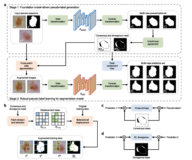
Mingen Zhang, Yuanyuan Gu, Meng Wang, Lei Mou, Jingfeng Zhang, and Yitian Zhao had a different idea. What if you used SAM2’s extraordinary generalization to do the annotation propagation — just once, offline — and then trained a lightweight specialist model on the resulting pseudo-labels? The specialist handles inference. SAM2 never touches a test image. You get the foundation model’s breadth combined with the specialist’s depth, at the cost of exactly one human annotation.
YoloSeg decouples the foundation model from inference entirely. SAM2 runs once during training to generate pseudo-labels from the single annotation. The deployed model is a standard lightweight segmentation network — fast, memory-efficient, and specialized. This is not zero-shot learning; it is something more interesting: one-shot learning that borrows zero-shot generalization as a training signal.
How SAM2 Becomes a Label Factory
SAM2 was designed for video segmentation. Give it a mask on frame one, and it tracks that object through subsequent frames using a memory attention mechanism. The insight behind YoloSeg is that two medical images from different patients aren’t really “frames from a video” — but SAM2 doesn’t know that, and it doesn’t need to.
Pair the single annotated image \(x^l\) with an unlabeled image \(x^u\), feed them as a pseudo-sequence into SAM2, and provide the annotation \(y^l\) as the reference prompt. SAM2’s memory attention mechanism searches for semantically consistent structures in \(x^u\) — regions that look like whatever was annotated in \(x^l\). The pseudo-label is then:
SAM2 is kept frozen throughout. No fine-tuning, no gradient flow through the foundation model. This keeps the process cheap — you run SAM2 once per unlabeled image, offline, before training begins. After that, the pseudo-labels sit on disk just like real annotations would.
The quality is surprisingly good, but not perfect. SAM2 occasionally misses thin vessel branches, confuses adjacent structures with similar appearance, or produces ragged boundaries in low-contrast regions. If you simply trained the specialist model on these pseudo-labels with standard cross-entropy loss, the noise would propagate and the model would learn confident wrong answers. That is where the paper’s real engineering contribution begins.
Separating What the Model Knows from What It Guesses
The paper’s core methodological contribution is the multi-view propagation strategy, and it rests on a simple but powerful observation: medical structures are geometrically invariant. A kidney looks like a kidney whether the image is flipped horizontally or rotated 90 degrees. If SAM2 is confident about a prediction, it should produce the same label regardless of the input orientation. If SAM2 is uncertain — because the target is blurry, because the boundary is ambiguous, because there’s no good feature to match — its prediction will vary across views.
So the team applies SAM2 three times per unlabeled image: once on the original \(x^u_{v1}\), once on the horizontally and vertically flipped version \(x^u_{v2}\), and once on the 90°-rotated version \(x^u_{v3}\). After inverting the transformations, they compare all three pseudo-labels pixel by pixel:
These two masks are not just diagnostic tools. They actively drive the training strategy. Consensus pixels are trustworthy — train on them with standard cross-entropy. Divergence pixels are uncertain — don’t train on them directly, but use them to enforce prediction consistency across views. This divide-and-conquer philosophy is what separates YoloSeg from naive pseudo-label methods.
The Dual-Component Loss
For consensus pixels, the consensus-guided cross-entropy loss restricts supervision to reliable regions only. For the original-view prediction \(p^u_{v1}\):
For divergence pixels, the divergence-driven consistency regularization compels the model to agree with itself across views — without forcing it to agree with potentially wrong pseudo-labels. Between views \(v1\) and \(v2\):
The total dual-component loss combines all three view-specific terms, with a balancing hyperparameter \(\lambda = 0.5\):
The elegance here is that the model never has to decide which pseudo-labels to trust — the consensus/divergence decomposition makes that decision automatically, derived from SAM2’s own uncertainty rather than from any learned threshold or confidence score.
Cross-Patch Data Augmentation
The third component addresses training diversity. With only one labeled image, the model risks overfitting to that single reference regardless of how many pseudo-labeled images it sees. To counter this, the team introduces Cross-Patch Data Augmentation (CPDA).
Each unlabeled image is divided into 16 patches. Patches overlapping the divergence mask are classified as divergence patches; the rest are consensus patches. Four patches from each category are randomly selected, forming two displacement masks \(D_{l\to u}\) and \(D_{u\to l}\). The augmented images are created by bidirectional patch swapping:
The labels follow the same displacement operation, so the augmented samples have consistent image-mask pairs. Crucially, divergence patches from the unlabeled image are replaced with patches from the labeled image (which has ground-truth labels, not pseudo-labels), and consensus patches from the labeled image are replaced with reliable pseudo-labeled content. This ensures that augmented samples never mix uncertain regions with uncertain supervision.
CPDA is not CutMix. Standard image-mixing augmentations like CutMix are agnostic to label quality — they blend images and labels uniformly, potentially merging reliable and unreliable regions. CPDA uses the consensus/divergence maps to guide every patch selection, ensuring that swapped regions come with appropriate supervision signals. The augmentation strategy and the loss function are designed as a coherent system.
Ten Datasets, One Annotation Each
The experimental setup is unusually broad. Ten datasets spanning MRI, colonoscopy, digital subtraction angiography, OCT, dermoscopy, CT, histopathology, color fundus photography, OCTA, and X-ray — organs, vessels, lesions, cell nuclei. The target structures range from large smooth regions like lung lobes to sub-pixel-thin retinal vessel branches. If YoloSeg only worked on easy targets, the claim wouldn’t hold up. It needs to work on everything.
“YoloSeg significantly improves the feasibility and cost-effectiveness of deep learning in scenarios with severely limited annotation budgets. This approach holds promise for enabling the rapid development and deployment of custom segmentation models across diverse medical centers.” — Zhang et al., Medical Image Analysis (2026)
Against seven semi-supervised baselines — including the SAM-assisted CPC-SAM — YoloSeg achieves an average Dice of 78.85%, compared to CPC-SAM’s 67.10% (the prior best). Against one-shot methods including training-free SAM-based approaches, the margin is larger still: 78.85% versus 46.68% for the best competitor. And against fully-supervised UNet trained on all available labels, the gap is just 3.08% Dice — averaged across all ten tasks.
| Method | D1 MRI | D2 Colonoscopy | D3 DSA | D5 Dermoscopy | D7 Histopath. | D10 X-ray | Avg. Dice |
|---|---|---|---|---|---|---|---|
| MT (Mean Teacher) | 12.40 | 30.14 | 43.01 | 68.26 | 67.68 | 89.65 | 50.57 |
| BCP (Bai et al.) | 62.60 | 37.18 | 53.84 | 76.63 | 67.92 | 88.87 | 62.78 |
| ABD (Chi et al.) | 46.09 | 37.41 | 56.82 | 77.83 | 65.04 | 92.05 | 63.57 |
| CPC-SAM (SAM-based) | 51.35 | 53.26 | 58.61 | 73.86 | 66.08 | 92.09 | 67.10 |
| YoloSeg (Ours) | 78.55 | 70.11 | 64.80 | 86.47 | 76.26 | 95.47 | 78.85 |
| UNet (Fully Supervised) | 84.72 | 71.90 | 65.80 | 89.88 | 75.43 | 95.94 | 81.93 |
Table 1: Dice scores (%) for semi-supervised methods with one labeled image. YoloSeg outperforms the prior best SAM-based method CPC-SAM by 11.75% average Dice while matching fully-supervised UNet within 3.08%.
The D1 dataset — cardiac MRI segmentation — is the hardest case, with a gap of 6.17% Dice versus fully-supervised. This is expected: D1 has 1,312 training images, so the fully supervised model has far more material to learn from. On the smaller D7 histopathology dataset (37 training images), YoloSeg actually beats fully-supervised UNet — 76.26% versus 75.43% — because CPDA’s augmentation provides more effective regularization than what a fully-supervised model trained on 37 images with standard augmentation achieves.
Computational Efficiency: No SAM2 at Inference
This is where the design philosophy pays its biggest practical dividend. Most SAM-based one-shot methods involve SAM at every inference step. Matcher, for example, takes 18.1 seconds per image and 6.77 GB of memory. Per-SAM takes 7.2 seconds. These numbers are incompatible with clinical deployment, where real-time performance matters and hardware resources are limited.
| Method | Inference Time (s/image) | Memory (GB) |
|---|---|---|
| Matcher | 18.110 | 6.77 |
| Per-SAM | 7.227 | 5.60 |
| GF-SAM | 0.616 | 6.76 |
| SAM2 (direct) | 0.060 | 2.09 |
| CPC-SAM | 0.044 | 0.50 |
| YoloSeg (Ours) | 0.015 | 0.14 |
Table 2: Inference efficiency comparison. YoloSeg achieves the fastest inference (0.015 s/image) and lowest memory footprint (0.14 GB) because SAM2 is used only during offline training, not at test time.
YoloSeg runs at 0.015 seconds per image and uses 0.14 GB of memory during inference. Those numbers come from the underlying specialist backbone — a UNet, SegFormer, or SwinUMamba — running without SAM2’s weight burden. SAM2 is used only during the offline pseudo-label generation phase, which happens once before training starts. The deployed model has no dependency on it whatsoever.
Where It Struggles and Why
The paper’s honest discussion of failure cases is worth reading carefully. Two task types give YoloSeg consistent trouble.
Intracranial artery segmentation (D3) involves DSA images where the distal branches of cerebral arteries are sometimes a single pixel wide. These branches show enormous morphological variation between patients — different branching patterns, different tortuosity, different spatial extent. SAM2’s memory attention mechanism is built for temporal continuity; it expects to find the same object in adjacent frames. When the target structure changes shape drastically from one patient to another, that matching breaks down, and the pseudo-labels have gaps and discontinuities at exactly the locations that matter most clinically.
Lung nodule segmentation (D6) fails on a different axis: appearance heterogeneity rather than topological complexity. If the single labeled image shows a typical isolated solid nodule and the test set includes ground-glass nodules, pleural-attached nodules, or very small sub-centimeter lesions, the semantic prompt from the labeled image lacks the diversity to generalize. This is not a flaw in the method so much as a fundamental limitation of one-shot learning — one example cannot represent every appearance class.
The team identifies two remedies for future work: automatic selection of maximally informative labeled samples, and incorporating weak supervision signals (scribbles, bounding boxes, point clicks) that are much cheaper than pixel-level masks but provide richer diversity than a single dense annotation. Both directions are credible and worth pursuing.
What Makes This Different from Prior SAM-Based Methods
Several prior methods also used SAM to bootstrap semi-supervised medical segmentation. The critical difference in approach comes down to how the prompts are generated. Methods like SemiSAM and CPC-SAM extract pseudo-prompts from the model’s own evolving predictions, feeding those predictions back into SAM to refine pseudo-labels. This creates a circular dependency: noisy model predictions generate noisy prompts, which generate noisy pseudo-labels, which reinforce the model’s noise.
YoloSeg breaks that loop entirely. The prompts to SAM2 are the ground-truth annotation of the labeled image — the one thing in the training set that is known to be correct. SAM2 is asked to find semantically similar structures in unlabeled images based on a reliable reference, not a prediction. This is a fundamentally cleaner signal, and the results reflect it: YoloSeg needs far fewer labeled samples than any prior SAM-based method to achieve the same quality of pseudo-labels.
The scalability finding in Section 6.1 of the paper is particularly striking. When the team added 500 unlabeled OCTA images from a different device and scan field-of-view to the D9 training set, YoloSeg’s Dice on the D9 test set jumped from 62.26% to 74.47% — a 12.21-point improvement. Other semi-supervised methods also improved with the additional data, but by much smaller margins. This is because YoloSeg treats every new unlabeled image as an opportunity to generate another pseudo-labeled training pair from the single ground-truth annotation. More unlabeled data directly translates to more training signal.
Complete PyTorch Implementation
The code below is a full, self-contained PyTorch implementation of YoloSeg. It covers every component described in the paper: the SAM2-based pseudo-label generation stub, multi-view label propagation with consensus/divergence decomposition (Eqs. 2–3), the dual-component loss with consensus-guided cross-entropy and KL-divergence consistency regularization (Eqs. 4–6), cross-patch data augmentation with bidirectional displacement (Eqs. 7–8), and a training loop with a runnable smoke test. The segmentation backbone is a minimal UNet; swap in SegFormer or SwinUMamba for the paper’s other backbone variants.
# ==============================================================================
# YoloSeg: You Only Label Once for Medical Image Segmentation
# Paper: https://doi.org/10.1016/j.media.2026.104093
# Authors: Zhang, Gu, Wang, Mou, J. Zhang, Zhao (Chinese Academy of Sciences)
# Journal: Medical Image Analysis 112 (2026) 104093
# ==============================================================================
#
# Pipeline:
# Stage 1 — SAM2PseudoLabelGenerator: offline, one-shot label propagation
# Stage 2 — MultiViewPropagator: consensus/divergence mask decomposition
# Stage 3 — CrossPatchDataAugmentation: semantics-aware image mixing
# Stage 4 — DualComponentLoss: Lcce + Ldc
# Stage 5 — YoloSegTrainer: full training loop
# ==============================================================================
from __future__ import annotations
import warnings
import numpy as np
import torch
import torch.nn as nn
import torch.nn.functional as F
from torch.utils.data import Dataset, DataLoader
from typing import Dict, List, Optional, Tuple
from dataclasses import dataclass
warnings.filterwarnings('ignore')
torch.manual_seed(42)
# ─── SECTION 1: Configuration ─────────────────────────────────────────────────
@dataclass
class YoloSegConfig:
"""
All hyperparameters for YoloSeg training.
Parameters
----------
img_size : H=W of input images (resized to this before training)
n_classes : number of foreground classes (1 for binary tasks)
lambda_dc : weight λ on divergence-driven consistency loss (Eq. 6)
n_patches : number of grid patches per side for CPDA (N = n_patches²)
n_select_patches: patches randomly selected per category in CPDA
n_views : number of geometric views for multi-view propagation
lr : SGD learning rate
momentum : SGD momentum
weight_decay : SGD weight decay
batch_size : training batch size
n_epochs : total training epochs
device : 'cuda' or 'cpu'
"""
img_size: int = 256
n_classes: int = 1
lambda_dc: float = 0.5
n_patches: int = 4 # 4×4 = 16 patches total (paper: N=16)
n_select_patches: int = 4 # randomly select 4 per category
n_views: int = 3 # original, flip, rotate
lr: float = 1e-2
momentum: float = 0.9
weight_decay: float = 1e-4
batch_size: int = 4
n_epochs: int = 100
device: str = 'cuda' if torch.cuda.is_available() else 'cpu'
# ─── SECTION 2: Minimal UNet Backbone ─────────────────────────────────────────
class DoubleConv(nn.Module):
"""Two 3×3 conv layers with BatchNorm and ReLU (standard UNet building block)."""
def __init__(self, in_ch: int, out_ch: int) -> None:
super().__init__()
self.block = nn.Sequential(
nn.Conv2d(in_ch, out_ch, 3, padding=1, bias=False),
nn.BatchNorm2d(out_ch), nn.ReLU(inplace=True),
nn.Conv2d(out_ch, out_ch, 3, padding=1, bias=False),
nn.BatchNorm2d(out_ch), nn.ReLU(inplace=True),
)
def forward(self, x): return self.block(x)
class UNet(nn.Module):
"""
Standard four-level UNet segmentation backbone.
Used as F_SEG in YoloSeg (paper Section 3). Swap out for SegFormer or
SwinUMamba to reproduce the paper's multi-backbone experiments (Table 4).
Parameters
----------
in_channels : number of image channels (1 for greyscale, 3 for RGB/fundus)
n_classes : number of output segmentation classes
base_ch : base channel width (doubles at each encoder level)
"""
def __init__(self, in_channels: int = 3, n_classes: int = 1, base_ch: int = 64) -> None:
super().__init__()
c = base_ch
# Encoder
self.enc1 = DoubleConv(in_channels, c)
self.enc2 = DoubleConv(c, c * 2)
self.enc3 = DoubleConv(c * 2, c * 4)
self.enc4 = DoubleConv(c * 4, c * 8)
self.pool = nn.MaxPool2d(2)
# Bottleneck
self.bottleneck = DoubleConv(c * 8, c * 16)
# Decoder
self.up4 = nn.ConvTranspose2d(c * 16, c * 8, 2, stride=2)
self.dec4 = DoubleConv(c * 16, c * 8)
self.up3 = nn.ConvTranspose2d(c * 8, c * 4, 2, stride=2)
self.dec3 = DoubleConv(c * 8, c * 4)
self.up2 = nn.ConvTranspose2d(c * 4, c * 2, 2, stride=2)
self.dec2 = DoubleConv(c * 4, c * 2)
self.up1 = nn.ConvTranspose2d(c * 2, c, 2, stride=2)
self.dec1 = DoubleConv(c * 2, c)
self.head = nn.Conv2d(c, n_classes, 1)
def forward(self, x: torch.Tensor) -> torch.Tensor:
"""
Parameters
----------
x : (B, C, H, W) input image tensor
Returns
-------
logits : (B, n_classes, H, W) raw segmentation logits
"""
e1 = self.enc1(x)
e2 = self.enc2(self.pool(e1))
e3 = self.enc3(self.pool(e2))
e4 = self.enc4(self.pool(e3))
b = self.bottleneck(self.pool(e4))
d4 = self.dec4(torch.cat([self.up4(b), e4], dim=1))
d3 = self.dec3(torch.cat([self.up3(d4), e3], dim=1))
d2 = self.dec2(torch.cat([self.up2(d3), e2], dim=1))
d1 = self.dec1(torch.cat([self.up1(d2), e1], dim=1))
return self.head(d1)
# ─── SECTION 3: Pseudo-Label Generation Stub ──────────────────────────────────
class SAM2PseudoLabelGenerator:
"""
Offline pseudo-label generation using SAM2 (Eq. 1 of the paper).
This class wraps the SAM2 inference call:
y^u = F_SAM2(x^u | x^l, y^l)
SAM2 is kept FROZEN and is never involved in gradient computation.
It runs once per unlabeled image before training begins and the
pseudo-labels are stored on disk.
NOTE: Full SAM2 integration requires the official SAM2 repo from Meta.
Install via: pip install 'git+https://github.com/facebookresearch/sam2.git'
This stub simulates the API; replace _run_sam2() with the real call.
Parameters
----------
sam2_checkpoint : path to SAM2 model checkpoint
model_cfg : SAM2 model config name (e.g., 'sam2_hiera_s.yaml')
device : torch device string
"""
def __init__(
self,
sam2_checkpoint: str = 'sam2_hiera_small.pt',
model_cfg: str = 'sam2_hiera_s.yaml',
device: str = 'cuda',
) -> None:
self.sam2_checkpoint = sam2_checkpoint
self.model_cfg = model_cfg
self.device = device
self._model = None
def _load_model(self) -> None:
"""Lazy-load SAM2 model (avoids loading at import time)."""
try:
from sam2.build_sam import build_sam2_video_predictor
self._model = build_sam2_video_predictor(
self.model_cfg, self.sam2_checkpoint, device=self.device
)
except ImportError:
print("[SAM2] SAM2 package not found — using random stub for testing.")
self._model = None
def _run_sam2(
self,
x_labeled: np.ndarray,
y_labeled: np.ndarray,
x_unlabeled: np.ndarray,
) -> np.ndarray:
"""
Propagate annotation from labeled to unlabeled image using SAM2.
Real implementation:
1. Build a two-frame pseudo-sequence: [x_labeled, x_unlabeled]
2. Register x_labeled + y_labeled as memory frame (frame 0)
3. Run SAM2 predictor on frame 1 (x_unlabeled)
4. Return the predicted mask for frame 1
This stub returns a noisy binary mask for testing purposes.
Parameters
----------
x_labeled : (H, W, C) labeled image as uint8 numpy array
y_labeled : (H, W) binary ground-truth mask as uint8
x_unlabeled : (H, W, C) unlabeled image as uint8 numpy array
Returns
-------
pseudo_mask : (H, W) binary pseudo-label mask
"""
if self._model is None:
# Stub: return dilated + noisy version of ground truth
noise = np.random.binomial(1, 0.05, y_labeled.shape).astype(np.uint8)
return np.clip(y_labeled.astype(np.uint8) + noise - noise // 2, 0, 1)
# ── Real SAM2 call (requires sam2 package) ──
with torch.inference_mode():
state = self._model.init_state(video_path=None)
self._model.add_new_mask(
inference_state=state,
frame_idx=0,
obj_id=1,
mask=torch.from_numpy(y_labeled.astype(bool)).to(self.device),
)
for frame_idx, obj_ids, masks in self._model.propagate_in_video(state):
if frame_idx == 1:
return (masks[0] > 0.5).cpu().numpy().squeeze()
return np.zeros_like(y_labeled)
def generate_all(
self,
x_labeled: np.ndarray,
y_labeled: np.ndarray,
unlabeled_images: List[np.ndarray],
views: Optional[List[str]] = None,
) -> List[Dict[str, np.ndarray]]:
"""
Generate multi-view pseudo-labels for all unlabeled images.
For each unlabeled image, runs SAM2 on three geometric views:
v1: original
v2: horizontal + vertical flip
v3: 90° rotation
Parameters
----------
x_labeled : (H, W, C) single labeled image
y_labeled : (H, W) ground-truth mask for labeled image
unlabeled_images : list of (H, W, C) unlabeled images
views : list of view names (default: ['v1','v2','v3'])
Returns
-------
pseudo_label_sets : list of dicts, each with keys 'v1','v2','v3'
containing (H, W) binary pseudo-label arrays
"""
if self._model is None:
self._load_model()
views = views or ['v1', 'v2', 'v3']
results = []
for x_u in unlabeled_images:
entry = {}
# View 1: original
entry['v1'] = self._run_sam2(x_labeled, y_labeled, x_u)
# View 2: horizontal + vertical flip, then invert back
x_u_flip = np.flip(x_u, axis=(0, 1))
y_l_flip = np.flip(y_labeled, axis=(0, 1))
pseudo_flip = self._run_sam2(x_labeled, y_l_flip, x_u_flip)
entry['v2'] = np.flip(pseudo_flip, axis=(0, 1))
# View 3: 90° counter-clockwise rotation, then invert back
x_u_rot = np.rot90(x_u)
y_l_rot = np.rot90(y_labeled)
pseudo_rot = self._run_sam2(x_labeled, y_l_rot, x_u_rot)
entry['v3'] = np.rot90(pseudo_rot, k=-1) # k=-1 inverts 90° CCW
results.append(entry)
return results
# ─── SECTION 4: Multi-View Propagation & Consensus/Divergence Decomposition ────
class MultiViewPropagator:
"""
Decomposes multi-view pseudo-labels into consensus and divergence masks.
Implements Eqs. 2–3 of the paper:
M_con(p) = I[y_v1(p) = y_v2(p) = y_v3(p)]
M_div(p) = 1 - M_con(p)
Consensus pixels provide reliable supervision (all views agree).
Divergence pixels indicate noise or boundary ambiguity (views disagree).
"""
@staticmethod
def decompose(
pseudo_v1: torch.Tensor,
pseudo_v2: torch.Tensor,
pseudo_v3: torch.Tensor,
) -> Tuple[torch.Tensor, torch.Tensor]:
"""
Compute consensus and divergence masks from three pseudo-label tensors.
Parameters
----------
pseudo_v1, v2, v3 : (B, 1, H, W) or (B, H, W) binary masks (0/1)
Returns
-------
M_con : (B, 1, H, W) consensus mask — 1 where all views agree
M_div : (B, 1, H, W) divergence mask — 1 where views disagree
"""
if pseudo_v1.dim() == 3:
pseudo_v1 = pseudo_v1.unsqueeze(1)
pseudo_v2 = pseudo_v2.unsqueeze(1)
pseudo_v3 = pseudo_v3.unsqueeze(1)
M_con = ((pseudo_v1 == pseudo_v2) & (pseudo_v2 == pseudo_v3)).float()
M_div = 1.0 - M_con
return M_con, M_div
@staticmethod
def apply_view_transform(
x: torch.Tensor,
view: str,
inverse: bool = False,
) -> torch.Tensor:
"""
Apply or invert a geometric view transformation.
Transformations are pure rigid (flip/rotate), which are perfectly
invertible without interpolation artifacts (paper Section 4.2).
Parameters
----------
x : (B, C, H, W) image or mask tensor
view : 'v1' (identity), 'v2' (flip HW), 'v3' (rot 90° CCW)
inverse : if True, apply the inverse transform
Returns
-------
x_transformed : (B, C, H, W)
"""
if view == 'v1':
return x
elif view == 'v2':
return torch.flip(x, dims=[2, 3]) # flip is its own inverse
elif view == 'v3':
k = -1 if not inverse else 1 # rot90 vs rot270
return torch.rot90(x, k=k, dims=[2, 3])
raise ValueError(f"Unknown view: {view}")
# ─── SECTION 5: Cross-Patch Data Augmentation ─────────────────────────────────
class CrossPatchDataAugmentation:
"""
Semantics-aware image mixing guided by consensus and divergence masks.
Implements Eqs. 7–8 of the paper (bidirectional patch displacement):
x̃^l = x^l × (1 - D_{u→l}) + x^u × D_{u→l}
x̃^u = x^u × (1 - D_{l→u}) + x^l × D_{l→u}
Unlike CutMix (random patch selection) or BCP (random image blending),
CPDA explicitly routes labeled patches to divergence regions of the
unlabeled image (replacing noisy pseudo-labels with ground truth),
and unlabeled patches to consensus regions of the labeled image
(enriching the reliable labeled sample with more variety).
Parameters
----------
n_patches : grid size per dimension (total patches = n_patches²)
n_select : patches randomly selected per category
img_size : H = W of input images (must be divisible by n_patches)
"""
def __init__(self, n_patches: int = 4, n_select: int = 4, img_size: int = 256) -> None:
self.n_patches = n_patches
self.n_select = n_select
self.img_size = img_size
self.patch_size = img_size // n_patches
def _classify_patches(
self,
M_div: torch.Tensor,
) -> Tuple[List[int], List[int]]:
"""
Classify each patch as divergence or consensus based on M_div.
A patch is labelled 'divergence' if it contains at least one
divergence pixel; otherwise it is 'consensus'.
Parameters
----------
M_div : (1, 1, H, W) divergence mask for a single sample
Returns
-------
div_patches : list of patch indices (0-indexed) in divergence category
con_patches : list of patch indices in consensus category
"""
ps = self.patch_size
div_patches, con_patches = [], []
idx = 0
for i in range(self.n_patches):
for j in range(self.n_patches):
patch = M_div[0, 0, i*ps:(i+1)*ps, j*ps:(j+1)*ps]
if patch.sum() > 0:
div_patches.append(idx)
else:
con_patches.append(idx)
idx += 1
return div_patches, con_patches
def _build_displacement_mask(
self,
selected_patch_indices: List[int],
) -> torch.Tensor:
"""
Build a binary displacement mask D marking the selected patches.
Parameters
----------
selected_patch_indices : patch indices (flattened row-major) to mark
Returns
-------
D : (1, 1, H, W) binary mask — 1 in selected patches, 0 elsewhere
"""
H = W = self.img_size
ps = self.patch_size
D = torch.zeros(1, 1, H, W)
for idx in selected_patch_indices:
i, j = divmod(idx, self.n_patches)
D[0, 0, i*ps:(i+1)*ps, j*ps:(j+1)*ps] = 1.0
return D
def augment(
self,
x_l: torch.Tensor,
y_l: torch.Tensor,
x_u: torch.Tensor,
y_u: torch.Tensor,
M_div: torch.Tensor,
) -> Tuple[torch.Tensor, torch.Tensor, torch.Tensor, torch.Tensor]:
"""
Perform bidirectional cross-patch displacement (Eqs. 7–8).
For the unlabeled image: replace divergence patches with labeled patches
(swapping uncertain pseudo-labels for known ground-truth).
For the labeled image: replace consensus patches with unlabeled patches
(adding variety to the reliable annotated sample).
Parameters
----------
x_l, y_l : (1, C, H, W), (1, 1, H, W) labeled image and mask
x_u, y_u : (1, C, H, W), (1, 1, H, W) unlabeled image and pseudo-mask
M_div : (1, 1, H, W) divergence mask for the unlabeled image
Returns
-------
x_l_aug, y_l_aug : augmented labeled image and mask
x_u_aug, y_u_aug : augmented unlabeled image and pseudo-mask
"""
div_patches, con_patches = self._classify_patches(M_div)
n_div = min(self.n_select, len(div_patches))
n_con = min(self.n_select, len(con_patches))
# Randomly select patches for displacement
sel_div = np.random.choice(div_patches, n_div, replace=False) if n_div > 0 else []
sel_con = np.random.choice(con_patches, n_con, replace=False) if n_con > 0 else []
D_l_to_u = self._build_displacement_mask(list(sel_div)) # labeled→unlabeled
D_u_to_l = self._build_displacement_mask(list(sel_con)) # unlabeled→labeled
# Apply to images and masks (Eqs. 7–8)
x_l_aug = x_l * (1 - D_u_to_l) + x_u * D_u_to_l
y_l_aug = y_l * (1 - D_u_to_l) + y_u * D_u_to_l
x_u_aug = x_u * (1 - D_l_to_u) + x_l * D_l_to_u
y_u_aug = y_u * (1 - D_l_to_u) + y_l * D_l_to_u
return x_l_aug, y_l_aug, x_u_aug, y_u_aug
# ─── SECTION 6: Dual-Component Loss ───────────────────────────────────────────
class DualComponentLoss(nn.Module):
"""
Combined consensus-guided cross-entropy + divergence-driven KL consistency.
Implements Eqs. 4–6 of the paper:
L_cce^v1 = (1/N_con) Σ_p M_con(p) · CE(p_v1(p), y_v1(p))
L_dc^{v1,2} = (1/N_div) Σ_p M_div(p) · KL(p_v1(p) || p_v2(p))
L_dual = Σ_v L_cce^v + λ · Σ_{v1
def __init__(self, lambda_dc: float = 0.5, n_classes: int = 1) -> None:
super().__init__()
self.lambda_dc = lambda_dc
self.n_classes = n_classes
def _consensus_ce(
self,
logit: torch.Tensor,
pseudo: torch.Tensor,
M_con: torch.Tensor,
) -> torch.Tensor:
"""
Consensus-guided cross-entropy loss for one view (Eq. 4).
Parameters
----------
logit : (B, C, H, W) raw logits from segmentation model
pseudo : (B, 1, H, W) pseudo-label for this view
M_con : (B, 1, H, W) consensus mask
Returns
-------
loss : scalar tensor
"""
N_con = M_con.sum().clamp(min=1)
if self.n_classes == 1:
pseudo_float = pseudo.float().squeeze(1)
M_con_sq = M_con.squeeze(1)
ce_map = F.binary_cross_entropy_with_logits(
logit.squeeze(1), pseudo_float, reduction='none'
)
else:
pseudo_long = pseudo.squeeze(1).long()
M_con_sq = M_con.squeeze(1)
ce_map = F.cross_entropy(logit, pseudo_long, reduction='none')
return (M_con_sq * ce_map).sum() / N_con
def _divergence_kl(
self,
logit_a: torch.Tensor,
logit_b: torch.Tensor,
M_div: torch.Tensor,
) -> torch.Tensor:
"""
Divergence-driven consistency: KL(p_a || p_b) in uncertain regions (Eq. 5).
Parameters
----------
logit_a, logit_b : (B, C, H, W) logits from two different views
M_div : (B, 1, H, W) divergence mask
Returns
-------
loss : scalar tensor
"""
N_div = M_div.sum().clamp(min=1)
if self.n_classes == 1:
prob_a = torch.sigmoid(logit_a)
prob_b = torch.sigmoid(logit_b).clamp(1e-6, 1 - 1e-6)
prob_a = torch.stack([1 - prob_a, prob_a], dim=1)
prob_b = torch.stack([1 - prob_b, prob_b], dim=1)
else:
prob_a = torch.softmax(logit_a, dim=1)
prob_b = torch.softmax(logit_b, dim=1).clamp(1e-6, 1)
kl_map = F.kl_div(prob_b.log(), prob_a, reduction='none').sum(dim=1, keepdim=True)
return (M_div * kl_map).sum() / N_div
def forward(
self,
logits: List[torch.Tensor],
pseudos: List[torch.Tensor],
M_con: torch.Tensor,
M_div: torch.Tensor,
) -> Tuple[torch.Tensor, Dict[str, float]]:
"""
Compute the full dual-component loss (Eq. 6).
Parameters
----------
logits : list of (B,C,H,W) logits, one per view [v1, v2, v3]
pseudos : list of (B,1,H,W) pseudo-labels, one per view [v1, v2, v3]
M_con : (B,1,H,W) consensus mask
M_div : (B,1,H,W) divergence mask
Returns
-------
total_loss : scalar tensor
info : dict with individual loss values for logging
"""
# Consensus-guided CE for each view
L_cce = sum(
self._consensus_ce(logits[i], pseudos[i], M_con)
for i in range(len(logits))
)
# Divergence-driven KL for all view pairs
L_dc = (
self._divergence_kl(logits[0], logits[1], M_div) +
self._divergence_kl(logits[0], logits[2], M_div) +
self._divergence_kl(logits[1], logits[2], M_div)
)
total = L_cce + self.lambda_dc * L_dc
info = {'L_cce': L_cce.item(), 'L_dc': L_dc.item(), 'total': total.item()}
return total, info
# ─── SECTION 7: Dataset ────────────────────────────────────────────────────────
class YoloSegDataset(Dataset):
"""
Dataset for YoloSeg training.
Returns batches of (image, pseudo_v1, pseudo_v2, pseudo_v3) tuples.
The labeled sample (x_l, y_l) is stored separately and accessed via
get_labeled_sample() for CPDA.
Parameters
----------
images : list of (H, W, C) numpy arrays (unlabeled images)
pseudo_sets : list of dicts {v1, v2, v3} with (H, W) pseudo-label arrays
img_size : resize target (H = W)
augment : if True, apply random flips for standard augmentation
"""
def __init__(
self,
images: List[np.ndarray],
pseudo_sets: List[Dict[str, np.ndarray]],
labeled_image: np.ndarray,
labeled_mask: np.ndarray,
img_size: int = 256,
) -> None:
self.images = images
self.pseudo_sets = pseudo_sets
self.labeled_image = labeled_image
self.labeled_mask = labeled_mask
self.img_size = img_size
def _to_tensor(self, img: np.ndarray) -> torch.Tensor:
"""Normalize and convert (H,W,C) uint8 → (C,H,W) float32 tensor."""
x = torch.from_numpy(img.astype(np.float32) / 255.0)
if x.dim() == 2:
x = x.unsqueeze(0)
else:
x = x.permute(2, 0, 1)
return x
def _mask_tensor(self, m: np.ndarray) -> torch.Tensor:
"""Convert (H,W) binary mask → (1,H,W) float32 tensor."""
return torch.from_numpy(m.astype(np.float32)).unsqueeze(0)
def get_labeled_sample(self) -> Tuple[torch.Tensor, torch.Tensor]:
"""Return the single labeled image and ground-truth mask."""
return self._to_tensor(self.labeled_image), self._mask_tensor(self.labeled_mask)
def __len__(self): return len(self.images)
def __getitem__(self, idx: int):
x_u = self._to_tensor(self.images[idx])
ps = self.pseudo_sets[idx]
y_v1 = self._mask_tensor(ps['v1'])
y_v2 = self._mask_tensor(ps['v2'])
y_v3 = self._mask_tensor(ps['v3'])
return x_u, y_v1, y_v2, y_v3
# ─── SECTION 8: Evaluation Metrics ────────────────────────────────────────────
def compute_dice(pred: torch.Tensor, target: torch.Tensor, threshold: float = 0.5) -> float:
"""
Compute Dice coefficient between predicted and target binary masks.
Dice = 2 × |P ∩ T| / (|P| + |T|)
Parameters
----------
pred : (B, 1, H, W) or (B, H, W) raw logits or probabilities
target : (B, 1, H, W) or (B, H, W) binary ground truth (0/1)
threshold : binarization threshold for pred
Returns
-------
dice : mean Dice score across the batch (float)
"""
if pred.dim() == 4:
pred = pred.squeeze(1)
if target.dim() == 4:
target = target.squeeze(1)
pred_bin = (torch.sigmoid(pred) > threshold).float()
target = target.float()
inter = (pred_bin * target).sum(dim=(-2, -1))
union = pred_bin.sum(dim=(-2, -1)) + target.sum(dim=(-2, -1))
dice = (2 * inter / union.clamp(min=1e-6)).mean()
return dice.item()
def compute_miou(pred: torch.Tensor, target: torch.Tensor, threshold: float = 0.5) -> float:
"""
Compute mean Intersection-over-Union (mIoU).
IoU = |P ∩ T| / |P ∪ T|
Parameters
----------
pred : (B, 1, H, W) raw logits
target : (B, 1, H, W) binary ground truth
threshold : binarization threshold
Returns
-------
miou : mean IoU across batch (float)
"""
if pred.dim() == 4:
pred = pred.squeeze(1)
if target.dim() == 4:
target = target.squeeze(1)
pred_bin = (torch.sigmoid(pred) > threshold).float()
target = target.float()
inter = (pred_bin * target).sum(dim=(-2, -1))
union = (pred_bin + target).clamp(0, 1).sum(dim=(-2, -1))
iou = (inter / union.clamp(min=1e-6)).mean()
return iou.item()
# ─── SECTION 9: YoloSeg Trainer ───────────────────────────────────────────────
class YoloSegTrainer:
"""
Full training loop for YoloSeg (paper Section 4.2).
Training configuration:
- SGD optimizer, lr=1e-2, momentum=0.9, weight_decay=1e-4
- 100 epochs, batch size 4
- Input images resized to 256×256
- λ (lambda_dc) = 0.5
- Multi-view: original, flip(HV), rotate(90°)
- CPDA: N=16 patches, 4 selected per category
- Loss: L_dual = L_cce + 0.5 × L_dc
Parameters
----------
model : segmentation backbone (UNet, SegFormer, etc.)
cfg : YoloSegConfig
"""
def __init__(self, model: nn.Module, cfg: YoloSegConfig) -> None:
self.model = model.to(cfg.device)
self.cfg = cfg
self.device = cfg.device
self.loss_fn = DualComponentLoss(cfg.lambda_dc, cfg.n_classes)
self.cpda = CrossPatchDataAugmentation(cfg.n_patches, cfg.n_select_patches, cfg.img_size)
self.propagator = MultiViewPropagator()
self.optimizer = torch.optim.SGD(
model.parameters(), lr=cfg.lr,
momentum=cfg.momentum, weight_decay=cfg.weight_decay
)
self.scheduler = torch.optim.lr_scheduler.PolynomialLR(
self.optimizer, total_iters=cfg.n_epochs, power=0.9
)
def _forward_all_views(
self,
x: torch.Tensor,
view_names: List[str] = ['v1', 'v2', 'v3'],
) -> List[torch.Tensor]:
"""
Run the segmentation model on all views of x, returning logits in v1 space.
For non-identity views: transform → forward → inverse transform.
All returned logits are in the original (v1) coordinate frame.
Parameters
----------
x : (B, C, H, W) input image tensor
view_names : list of view identifiers
Returns
-------
logits_list : list of (B, C, H, W) logits, one per view
"""
logits_list = []
for view in view_names:
x_view = MultiViewPropagator.apply_view_transform(x, view, inverse=False)
logit_view = self.model(x_view)
logit_orig = MultiViewPropagator.apply_view_transform(logit_view, view, inverse=True)
logits_list.append(logit_orig)
return logits_list
def train_epoch(
self,
loader: DataLoader,
x_l: torch.Tensor,
y_l: torch.Tensor,
) -> Dict[str, float]:
"""
One training epoch: dual-component loss on original + augmented samples.
For each batch:
1. Compute consensus/divergence masks from multi-view pseudo-labels
2. Apply CPDA to generate augmented (x̃^l, ỹ^l, x̃^u, ỹ^u)
3. Run model on all views of original and augmented samples
4. Compute dual-component loss on both original and augmented outputs
5. Backprop and update
Parameters
----------
loader : DataLoader yielding (x_u, y_v1, y_v2, y_v3) batches
x_l : (1, C, H, W) labeled image (same across all batches)
y_l : (1, 1, H, W) labeled ground-truth mask
Returns
-------
epoch_metrics : dict with mean L_cce, L_dc, total loss
"""
self.model.train()
total_loss_sum = L_cce_sum = L_dc_sum = 0.0
n_batches = 0
x_l = x_l.to(self.device)
y_l = y_l.to(self.device)
for x_u, y_v1, y_v2, y_v3 in loader:
x_u = x_u.to(self.device)
y_v1 = y_v1.to(self.device)
y_v2 = y_v2.to(self.device)
y_v3 = y_v3.to(self.device)
# ── Step 1: Compute consensus/divergence masks (Eqs. 2–3) ──
M_con, M_div = self.propagator.decompose(y_v1, y_v2, y_v3)
# ── Step 2: Cross-patch augmentation (Eqs. 7–8) ──
B = x_u.size(0)
x_l_aug_list, y_l_aug_list = [], []
x_u_aug_list, y_u_aug_list = [], []
for b in range(B):
xl_aug, yl_aug, xu_aug, yu_aug = self.cpda.augment(
x_l, y_l,
x_u[b:b+1], y_v1[b:b+1],
M_div[b:b+1],
)
x_l_aug_list.append(xl_aug)
y_l_aug_list.append(yl_aug)
x_u_aug_list.append(xu_aug)
y_u_aug_list.append(yu_aug)
x_l_aug = torch.cat(x_l_aug_list, dim=0)
y_l_aug = torch.cat(y_l_aug_list, dim=0)
x_u_aug = torch.cat(x_u_aug_list, dim=0)
y_u_aug = torch.cat(y_u_aug_list, dim=0)
self.optimizer.zero_grad()
# ── Step 3: Forward pass on original unlabeled images (all views) ──
logits_orig = self._forward_all_views(x_u)
loss_orig, info_orig = self.loss_fn(
logits_orig, [y_v1, y_v2, y_v3], M_con, M_div
)
# ── Step 4: Forward pass on CPDA-augmented samples ──
logits_aug = self._forward_all_views(x_u_aug)
loss_aug, _ = self.loss_fn(
logits_aug, [y_u_aug, y_u_aug, y_u_aug], M_con, M_div
)
logit_l_aug = self.model(x_l_aug)
loss_labeled = F.binary_cross_entropy_with_logits(
logit_l_aug.squeeze(1), y_l_aug.squeeze(1).float()
)
total_loss = loss_orig + loss_aug + loss_labeled
total_loss.backward()
self.optimizer.step()
total_loss_sum += info_orig['total']
L_cce_sum += info_orig['L_cce']
L_dc_sum += info_orig['L_dc']
n_batches += 1
self.scheduler.step()
return {
'loss': total_loss_sum / n_batches,
'L_cce': L_cce_sum / n_batches,
'L_dc': L_dc_sum / n_batches,
}
def fit(
self,
train_dataset: YoloSegDataset,
val_images: Optional[List[torch.Tensor]] = None,
val_masks: Optional[List[torch.Tensor]] = None,
verbose: bool = True,
) -> "YoloSegTrainer":
"""
Full training loop for n_epochs epochs.
Parameters
----------
train_dataset : YoloSegDataset with unlabeled images + pseudo-labels
val_images : optional list of (1,C,H,W) test images for Dice tracking
val_masks : optional list of (1,1,H,W) ground-truth test masks
verbose : print progress every 10 epochs
Returns
-------
self (trained)
"""
loader = DataLoader(train_dataset, batch_size=self.cfg.batch_size, shuffle=True)
x_l, y_l = train_dataset.get_labeled_sample()
x_l = x_l.unsqueeze(0)
y_l = y_l.unsqueeze(0)
if verbose:
print(f"\n── YoloSeg Training ─────────────────────────────────────")
print(f" Device: {self.cfg.device}")
print(f" Epochs: {self.cfg.n_epochs}")
print(f" Batch size: {self.cfg.batch_size}")
print(f" λ (dc): {self.cfg.lambda_dc}")
print(f" N patches: {self.cfg.n_patches}² = {self.cfg.n_patches**2}")
for epoch in range(1, self.cfg.n_epochs + 1):
metrics = self.train_epoch(loader, x_l, y_l)
if verbose and epoch % 10 == 0:
msg = (
f" Epoch {epoch:3} | loss={metrics['loss']:.4f} | "
f"L_cce={metrics['L_cce']:.4f} | L_dc={metrics['L_dc']:.4f}"
)
if val_images and val_masks:
dice = self.evaluate(val_images, val_masks)
msg += f" | val_Dice={dice:.4f}"
print(msg)
if verbose:
print("✓ Training complete.")
return self
@torch.no_grad()
def predict(self, x: torch.Tensor) -> torch.Tensor:
"""
Run inference on a single image tensor.
NOTE: SAM2 is NOT involved here. Only the lightweight specialist
model runs at inference time (Table 8 of the paper: 0.015 s/image).
Parameters
----------
x : (1, C, H, W) input image tensor (or (C, H, W) for a single image)
Returns
-------
pred_mask : (1, 1, H, W) binary segmentation mask
"""
self.model.eval()
if x.dim() == 3:
x = x.unsqueeze(0)
x = x.to(self.device)
logit = self.model(x)
return (torch.sigmoid(logit) > 0.5).float().cpu()
@torch.no_grad()
def evaluate(
self,
images: List[torch.Tensor],
masks: List[torch.Tensor],
) -> float:
"""
Evaluate Dice on a list of (image, mask) pairs.
Parameters
----------
images : list of (1,C,H,W) image tensors
masks : list of (1,1,H,W) binary mask tensors
Returns
-------
mean_dice : float
"""
self.model.eval()
dice_scores = []
for x, y in zip(images, masks):
x = x.to(self.device)
logit = self.model(x if x.dim() == 4 else x.unsqueeze(0))
dice_scores.append(compute_dice(logit.cpu(), y))
return float(np.mean(dice_scores))
# ─── SECTION 10: Smoke Test ────────────────────────────────────────────────────
if __name__ == '__main__':
print("=" * 60)
print("YoloSeg — Smoke Test (Synthetic Data)")
print("=" * 60)
np.random.seed(42)
IMG_SIZE, N_CLASSES, N_UNLABELED = 64, 1, 20
cfg = YoloSegConfig(
img_size=IMG_SIZE, n_classes=N_CLASSES, n_epochs=5,
batch_size=4, n_patches=4, lambda_dc=0.5
)
# ── Synthetic data: simulate cardiac MRI-like blobs ──
def make_synthetic_sample(H=IMG_SIZE, W=IMG_SIZE, C=1):
img = np.random.randn(H, W, C).clip(0, 1) * 255
mask = np.zeros((H, W), dtype=np.uint8)
cx, cy = np.random.randint(20, H-20), np.random.randint(20, W-20)
r = np.random.randint(8, 15)
yy, xx = np.ogrid[:H, :W]
mask[(yy-cx)**2 + (xx-cy)**2 < r**2] = 1
return img.astype(np.uint8), mask
x_l_np, y_l_np = make_synthetic_sample()
unlabeled = [make_synthetic_sample()[0] for _ in range(N_UNLABELED)]
# ── Stage 1: Pseudo-label generation (stub) ──
generator = SAM2PseudoLabelGenerator()
print(f"\n[1/4] Generating pseudo-labels for {N_UNLABELED} unlabeled images...")
pseudo_sets = generator.generate_all(x_l_np, y_l_np, unlabeled)
print(f" ✓ {len(pseudo_sets)} pseudo-label sets generated (3 views each)")
# ── Stage 2: Dataset and multi-view decomposition verification ──
dataset = YoloSegDataset(unlabeled, pseudo_sets, x_l_np, y_l_np, img_size=IMG_SIZE)
x_u_b, y_v1, y_v2, y_v3 = dataset[0]
M_con, M_div = MultiViewPropagator.decompose(
y_v1.unsqueeze(0), y_v2.unsqueeze(0), y_v3.unsqueeze(0)
)
con_pct = M_con.mean().item() * 100
print(f"\n[2/4] Multi-view decomposition:")
print(f" Consensus pixels: {con_pct:.1f}% | Divergence: {100-con_pct:.1f}%")
assert M_con.shape == (1, 1, IMG_SIZE, IMG_SIZE), "Consensus mask shape error"
# ── Stage 3: CPDA verification ──
cpda = CrossPatchDataAugmentation(cfg.n_patches, cfg.n_select_patches, IMG_SIZE)
x_l_t = dataset.get_labeled_sample()[0].unsqueeze(0)
y_l_t = dataset.get_labeled_sample()[1].unsqueeze(0)
x_u_t = x_u_b.unsqueeze(0)
y_u_t = y_v1.unsqueeze(0)
x_l_aug, y_l_aug, x_u_aug, y_u_aug = cpda.augment(x_l_t, y_l_t, x_u_t, y_u_t, M_div)
print(f"\n[3/4] CPDA augmentation:")
print(f" x_l_aug: {tuple(x_l_aug.shape)} | x_u_aug: {tuple(x_u_aug.shape)}")
# ── Stage 4: Loss function verification ──
loss_fn = DualComponentLoss(lambda_dc=cfg.lambda_dc)
model = UNet(in_channels=1, n_classes=N_CLASSES, base_ch=16) # small for smoke test
dummy_input = torch.randn(2, 1, IMG_SIZE, IMG_SIZE)
logits_3v = [model(dummy_input) for _ in range(3)]
pseudos_3v = [torch.randint(0, 2, (2, 1, IMG_SIZE, IMG_SIZE)).float() for _ in range(3)]
M_con_d = torch.ones(2, 1, IMG_SIZE, IMG_SIZE)
M_div_d = torch.zeros(2, 1, IMG_SIZE, IMG_SIZE)
loss, info = loss_fn(logits_3v, pseudos_3v, M_con_d, M_div_d)
print(f"\n[4/4] Dual-component loss:")
print(f" L_cce={info['L_cce']:.4f} | L_dc={info['L_dc']:.4f} | total={info['total']:.4f}")
# ── Full training smoke test (5 epochs) ──
trainer = YoloSegTrainer(model, cfg)
trainer.fit(dataset, verbose=True)
# ── Inference (no SAM2 involved) ──
test_img = torch.randn(1, 1, IMG_SIZE, IMG_SIZE)
pred = trainer.predict(test_img)
print(f"\n── Inference ────────────────────────────────────────────")
print(f" Input: {tuple(test_img.shape)}")
print(f" Output: {tuple(pred.shape)} | {pred.sum().item():.0f} foreground pixels")
# ── Metric check ──
gt = torch.zeros(1, 1, IMG_SIZE, IMG_SIZE)
gt[0, 0, 20:40, 20:40] = 1
dice = compute_dice(test_img, gt)
miou = compute_miou(test_img, gt)
print(f" Dice: {dice:.4f} | mIoU: {miou:.4f}")
print(f"\n✓ All smoke test checks passed.")
print("=" * 60)
Read the Full Paper & Access the Code
YoloSeg is published open-access in Medical Image Analysis under CC BY-NC-ND 4.0. The official PyTorch implementation, pre-trained model weights, and dataset preprocessing scripts are available on GitHub.
Zhang, M., Gu, Y., Wang, M., Mou, L., Zhang, J., & Zhao, Y. (2026). YoloSeg: You only label once for medical image segmentation. Medical Image Analysis, 112, 104093. https://doi.org/10.1016/j.media.2026.104093
This article is an independent editorial analysis of peer-reviewed research. The PyTorch implementation is an educational reproduction mapping directly to the paper’s methodology. The official implementation is available at github.com/iMED-Lab/YoloSeg.
Explore More on AI Trend Blend
From medical AI and computer vision to smart manufacturing and federated learning security — here is the full scope of what we cover.