The Two Clocks That Fixed GAN Training: A Complete Theory of Two-Timescale Gradient Descent Ascent
Tianyi Lin, Chi Jin, and Michael I. Jordan from Columbia, Princeton, and UC Berkeley deliver the first rigorous nonasymptotic analysis of two-timescale gradient descent ascent — the algorithm that has powered GAN training in practice for years — establishing tight complexity bounds for four distinct settings, including the notoriously difficult nonsmooth case.
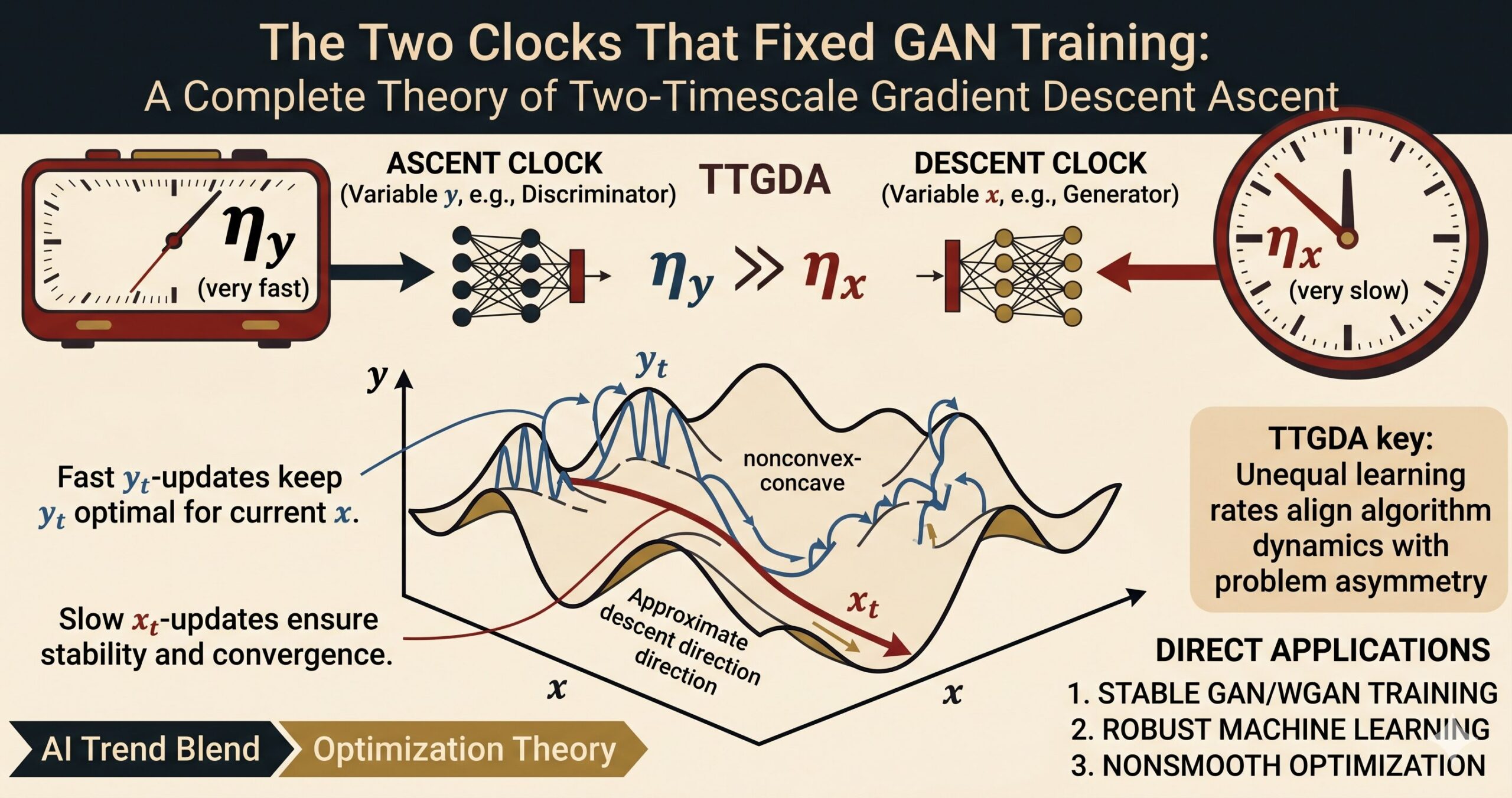
If you have ever trained a generative adversarial network, you have almost certainly tuned the learning rates for the generator and discriminator separately — and probably found that a larger discriminator learning rate makes everything run more smoothly. What you were doing, without necessarily knowing the name, was two-timescale gradient descent ascent. The method has been standard practice in GAN training since Heusel et al. (2017). What it lacked, until this paper, was a rigorous nonasymptotic convergence theory that could explain why it works, how fast it converges, and what happens when the objective function is not even smooth.
What Minimax Optimization Actually Is — and Why Single-Timescale GDA Breaks
The minimax problem is written compactly as:
Think of \(x\) as the generator parameters in a GAN and \(y\) as the discriminator parameters. The generator wants to minimise the adversarial loss; the discriminator wants to maximise it. In robust machine learning, \(x\) is a classifier and \(y\) parametrises the worst-case distribution — you train for robustness by finding the \(x\) that performs well even against the adversarially chosen \(y\).
The simplest algorithm is single-timescale gradient descent ascent (GDA): take one gradient descent step in \(x\) and one gradient ascent step in \(y\) with the same learning rate. This works beautifully when \(f\) is convex in \(x\) and concave in \(y\) — decades of theory guarantee convergence in that regime. But in the nonconvex settings that arise in actual deep learning, single-timescale GDA can cycle, oscillate, or diverge entirely. The empirical observation that separating the two learning rates — letting the \(y\)-update move faster than the \(x\)-update — stabilises training had no theoretical grounding in the nonconvex regime.
That is precisely the gap this paper fills. The two-timescale GDA (TTGDA) algorithm uses unequal learning rates \(\eta_x \ll \eta_y\), encoding the asymmetric structure of the problem: \(y\) needs to stay nearly optimal for the current \(x\), while \(x\) descends slowly enough that the inner maximisation problem can track it. The paper gives this intuition a precise mathematical form and derives the first nonasymptotic complexity bounds for all four practically relevant settings.
The asymmetry \(\eta_x \ll \eta_y\) matches the asymmetric structure of nonconvex-concave minimax problems. A fast \(y\)-update keeps \(y_t\) close to the optimal \(y^*(x_t)\) for the current \(x_t\), which means the gradient \(\nabla_x f(x_t, y_t)\) is a good approximation to \(\nabla \Phi(x_t)\) — the true descent direction for the outer minimisation. Slow down \(x\) and this approximation stays valid; speed it up and it breaks.
The Two Algorithms
TTGDA is the deterministic version: at each step, compute exact partial (sub)gradients \((g^t_x, g^t_y) \in \partial f(x^t, y^t)\), then update both variables simultaneously — \(x\) by gradient descent and \(y\) by projected gradient ascent onto the constraint set \(\mathcal{Y}\):
TTSGDA is the stochastic counterpart: instead of exact gradients, it averages \(M\) independent stochastic estimates at each step, where the estimator \(G = (G_x, G_y)\) is unbiased with bounded variance \(\sigma^2\):
The key design parameter is the ratio \(\eta_y / \eta_x\). In the nonconvex-strongly-concave setting this ratio is \(\Theta(\kappa^2)\); in the nonconvex-concave setting it grows to \(\Theta(\epsilon^{-4})\) — a dramatic asymmetry that reflects how much harder the inner maximisation becomes when strong concavity is absent.
What “Stationarity” Means When the Landscape Is Rough
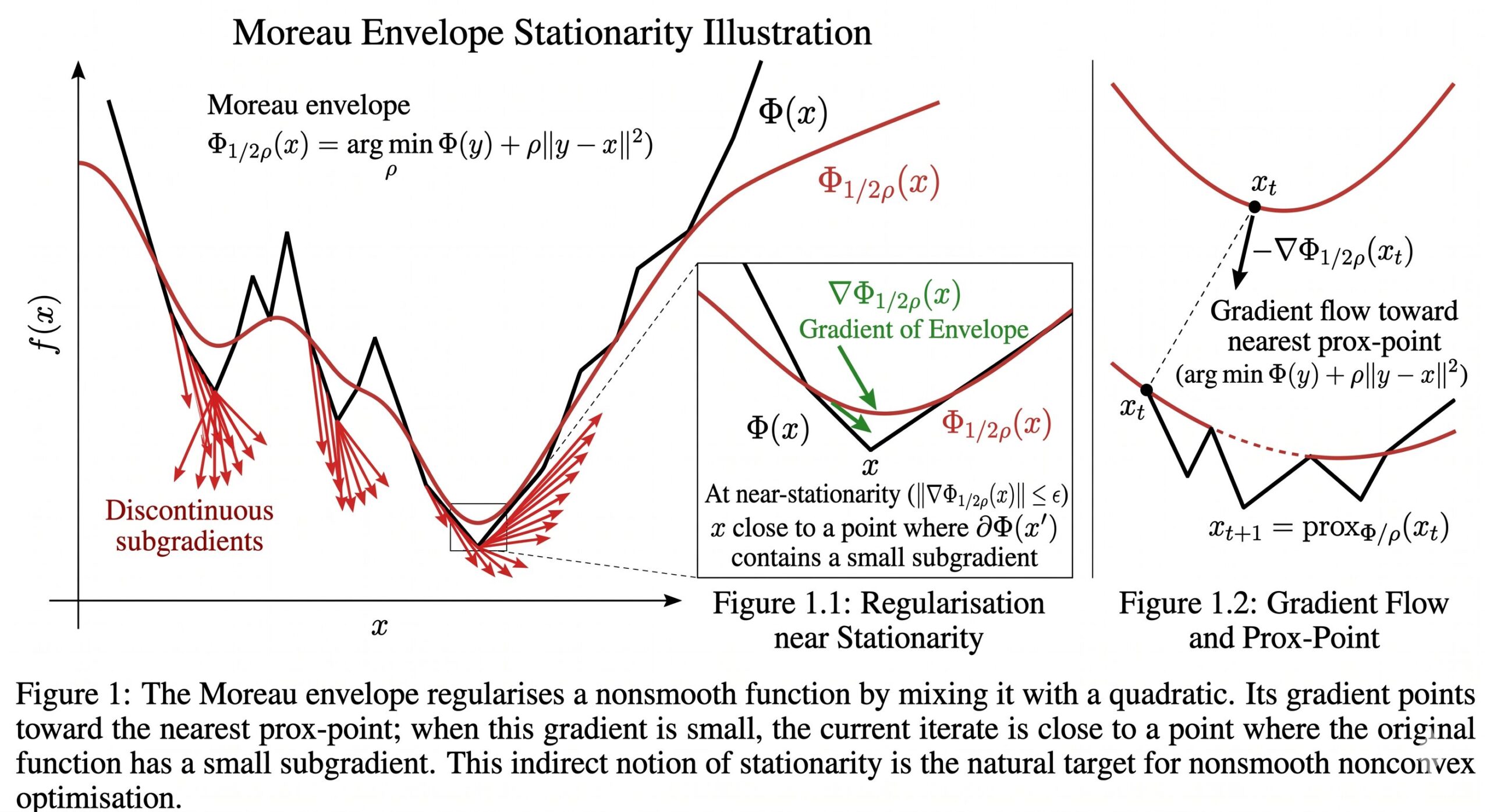
Before stating any convergence results, the paper carefully sets up the right notion of what counts as a “solution.” In smooth nonconvex optimisation, the natural target is a point where the gradient is small: \(\|\nabla \Phi(x)\| \leq \epsilon\). But in the settings this paper covers, the outer objective \(\Phi(x) = \max_{y \in \mathcal{Y}} f(x, y)\) may not even be differentiable.
The authors use the Moreau envelope \(\Phi_\lambda\) to define stationarity for nonsmooth settings. The Moreau envelope with parameter \(\lambda > 0\) is:
Two key properties make this useful. First, when \(\Phi\) is \(\rho\)-weakly convex, its Moreau envelope \(\Phi_{1/2\rho}\) is \(\rho\)-smooth — so it has a well-defined gradient. Second, that gradient has a clean closed form: \(\nabla \Phi_{1/2\rho}(x) = 2\rho(x – \text{prox}_{\Phi/2\rho}(x))\). A point where \(\|\nabla \Phi_{1/2\rho}(x)\| \leq \epsilon\) is guaranteed to be near a point with a small subgradient of \(\Phi\) itself — the two notions are equivalent up to a factor of \(\epsilon/2\rho\) in distance.
This is not merely a mathematical convenience. In adversarial machine learning, \(x\) is the classifier and \(y\) is the adversarial perturbation. Practitioners want a robust classifier — one that is an approximate stationary point of the outer objective — not an exact reconstruction of every adversarial example. The Moreau envelope stationarity captures exactly that.
Four Settings, Four Theorems
Setting 1: Smooth + Nonconvex-Strongly-Concave (Theorem 17)
When \(f\) is \(\ell\)-smooth and \(\mu\)-strongly concave in \(y\), the outer function \(\Phi\) is differentiable with Lipschitz gradient, and the condition number \(\kappa = \ell/\mu\) controls everything. With fixed learning rates \(\eta_x = 1/(16(\kappa+1)^2\ell)\) and \(\eta_y = 1/\ell\), TTGDA needs:
TTSGDA with batch size \(M = \max\{1, 48\kappa\sigma^2/\epsilon^2\}\) needs \(O(\kappa^2 \epsilon^{-2} \cdot \max\{1, \kappa\sigma^2/\epsilon^2\})\) stochastic gradient evaluations. The ratio \(\eta_y/\eta_x = \Theta(\kappa^2)\) is not a coincidence — it precisely reflects the algorithmic efficiency trade-off required to keep \(y_t\) close to \(y^*(x_t)\) while \(x_t\) descends.
Setting 2: Smooth + Nonconvex-Concave (Theorem 19)
Without strong concavity, the optimal \(y^*(x)\) is no longer unique and can jump discontinuously even when \(x\) moves smoothly. The ratio \(\eta_y/\eta_x\) must now scale as \(\Theta(\epsilon^{-4})\) — a stark reminder of how much harder the problem becomes. TTGDA with carefully chosen decaying stepsizes requires:
Here \(L\) is the Lipschitz constant of \(f\) in \(x\), \(D\) is the diameter of \(\mathcal{Y}\), and \(\Delta_0 = \Phi(x_0) – f(x_0, y_0)\) measures how far the initial \(y_0\) is from optimal. The \(\epsilon^{-6}\) scaling (in the regime where \(\ell^2 D^2/\epsilon^2 > 1\)) is the main cost of losing strong concavity.
Setting 3: Nonsmooth + Nonconvex-Strongly-Concave (Theorem 24)
Now \(f\) is only assumed to be \(L\)-Lipschitz and \(\rho\)-weakly convex in \(x\) — the kind of regularity satisfied by ReLU networks. The smooth gradient \(\nabla_x f\) no longer exists; instead the algorithm works with Clarke subgradients. A critical new ingredient is an adaptive stepsize schedule for \(y\): within each epoch, the \(y\)-learning rate decreases as \(\eta^t_y = 1/(\mu t)\), then resets at the start of the next epoch. This mimics the classical schedule for strongly convex subgradient methods and is necessary to control the error introduced by nonsmoothness.
The same \(O(\epsilon^{-4})\) base rate as the smooth strongly-concave case, but with a logarithmic factor that reflects the cost of the adaptive stepsize. Deterministic and stochastic algorithms achieve the same order — consistent with classical results in nonsmooth optimisation.
Setting 4: Nonsmooth + Nonconvex-Concave (Theorem 26)
The hardest setting: Lipschitz, weakly convex in \(x\), and only concave (not strongly) in \(y\). A fixed \(y\)-learning rate is used again, balanced against the \(x\)-rate through the condition \(\eta_y/\eta_x = \Theta(\epsilon^{-4})\):
These four theorems, taken together, form a complete map of the complexity landscape for TTGDA. The paper is honest that these bounds are not always optimal — nested-loop algorithms achieve better rates in some smooth settings — but TTGDA’s single-loop structure and simplicity make it vastly more practical to implement and tune.
Smooth strongly-concave: \(O(\kappa^2 \epsilon^{-2})\). Smooth concave: \(O(\epsilon^{-6})\). Nonsmooth strongly-concave: \(\tilde{O}(\epsilon^{-4})\). Nonsmooth concave: \(O(\epsilon^{-8})\). Each step down in structure (losing smoothness or strong concavity) costs roughly a factor of \(\epsilon^{-2}\) — a precise quantification of how much harder the problem becomes.
The Proof Technique: Slowly Changing Concave Problems
Standard analyses of nested-loop algorithms work by demanding that the inner variable \(y_t\) be kept close to \(y^*(x_t)\) — the exact optimum for the current \(x_t\) — at every step. This is enforced by running many inner iterations before taking any outer step. Applying this approach to TTGDA is problematic: in the nonconvex-concave setting, \(y^*(x)\) is not unique and can shift dramatically when \(x\) changes, so there is no guarantee that a single gradient ascent step keeps \(y_t\) close to \(y^*(x_t)\).
The paper’s innovation is to avoid tracking \(y^*(x_t)\) entirely. Instead, the authors define the gap \(\Delta_t = \Phi(x_t) – f(x_t, y_t)\) — how far the current \(y_t\) is from optimal in value, rather than in distance — and prove that a single gradient ascent step is sufficient to control the average of \(\Delta_t\) over time, even though \(y_t\) may never be close to \(y^*(x_t)\).
The key insight is that the objective \(f(x_t, \cdot)\) changes slowly: since \(x_t\) moves slowly (small \(\eta_x\)), the function \(\Phi(x_t) = \max_y f(x_t, y)\) also changes slowly (because \(\Phi\) is Lipschitz). One gradient ascent step with a well-chosen stepsize is enough to make progress against a slowly drifting concave target. This leads to a clean descent inequality for the Moreau envelope:
Summing this inequality over \(T+1\) steps and controlling \(\sum_t \Delta_t\) through the localization argument gives the final complexity bound. The argument is surprisingly clean compared to nested-loop analyses and extends naturally to all four settings by swapping the regularity assumptions.
Robust Logistic Regression and WGAN Training
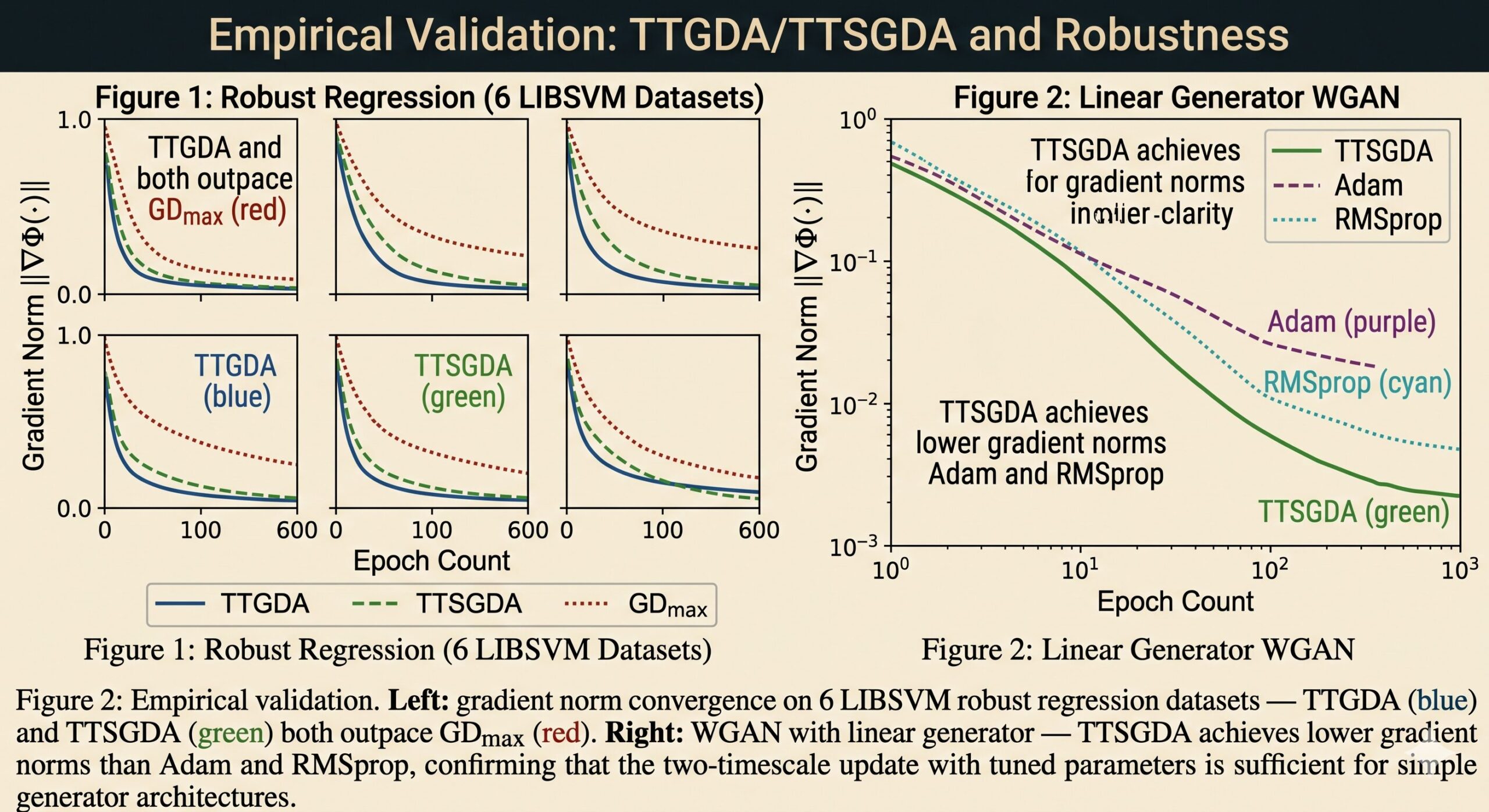
The paper validates TTGDA and TTSGDA on two application domains. The first is robust logistic regression with a nonconvex penalty, formulated as a minimax problem over six LIBSVM benchmark datasets. TTGDA and TTSGDA consistently converge faster than GDmax — the algorithm that solves the inner maximisation exactly at each step — across all six datasets, measured by the gradient norm of \(\Phi\). This confirms that the efficiency gained by skipping the exact inner solve is real, not just theoretical.
The second application is Wasserstein GAN training, tested with both linear and nonlinear generators. With a linear generator (simpler structure), TTSGDA outperforms both Adam and RMSprop. With a nonlinear ReLU generator (richer structure), TTSGDA in its vanilla form lags behind Adam and RMSprop — which are specifically engineered for handling the complex gradient landscape of deep networks. The authors are candid about this: the theoretical guarantees apply, but the vanilla implementation does not exploit the adaptive second-moment estimates that make Adam effective on highly nonlinear problems. Combining TTSGDA with adaptive regularisation is flagged as a natural extension.
How This Fits the Broader Minimax Landscape
The paper situates itself carefully in a crowded field. Several prior works achieved \(O(\epsilon^{-3})\) gradient evaluations for smooth nonconvex-concave problems using nested-loop algorithms — notably the ProxDIAG algorithm and the accelerated inexact proximal point method of Kong and Monteiro (2021). Those algorithms are more sample-efficient in theory but substantially more complex to implement, requiring an inner solver to be run to convergence at each outer step.
TTGDA achieves \(O(\epsilon^{-6})\) in the smooth nonconvex-concave setting — worse by a factor of \(\epsilon^{-3}\) — but it is a single-loop algorithm with no inner subroutine, no warm-starting, and no convergence criterion for a subproblem. For practitioners who want to set a learning rate, run SGD, and let it converge, TTGDA’s simplicity more than compensates for the theoretical gap.
In the nonsmooth settings, the paper is the first to establish anything at all. Prior work by Rafique et al. (2021) handled nonsmooth objectives but only for nested-loop algorithms. Boţ and Böhm (2023) studied alternating TTGDA in a partially nonsmooth setting — nonsmooth in \(x\) but smooth in \(y\) — and got the same complexity as the smooth case by exploiting the smoothness in \(y\). The current paper drops that smoothness assumption entirely, handling the truly nonsmooth case where both \(x\) and \(y\) updates involve subgradients. The cost is a factor of \(\epsilon^{-2}\) in complexity compared to the smooth counterpart, which the authors prove is unavoidable with the current technique.
“Our proof technique directly analyzes the concave optimization problem with a slowly changing objective function — rather than requiring \(y_t\) to stay close to \(y^*(x_t)\), it only requires the value gap \(\Delta_t\) to be controlled on average. This makes TTGDA tractable to analyze without any inner-loop subroutine.” — Lin, Jin and Jordan, JMLR (2025)
Complexity Summary Table
| Setting | Smoothness | Concavity in y | TTGDA (det.) | TTSGDA (stoch.) |
|---|---|---|---|---|
| S1 | \(\ell\)-smooth | \(\mu\)-strongly concave | \(O(\kappa^2 \epsilon^{-2})\) | \(O(\kappa^3 \epsilon^{-4})\) |
| S2 | \(\ell\)-smooth | Concave | \(O(\epsilon^{-6})\) | \(O(\epsilon^{-8})\) |
| S3 | Nonsmooth (\(\rho\)-weakly cvx) | \(\mu\)-strongly concave | \(\tilde{O}(\epsilon^{-4})\) | \(\tilde{O}(\epsilon^{-4})\) |
| S4 | Nonsmooth (\(\rho\)-weakly cvx) | Concave | \(O(\epsilon^{-8})\) | \(O(\epsilon^{-8})\) |
Table 1: Gradient evaluation complexity for TTGDA and TTSGDA across all four settings. \(\kappa = \ell/\mu\) is the condition number. The \(\tilde{O}\) notation hides logarithmic factors. Each step down in structure (losing smoothness or strong concavity) costs roughly \(\epsilon^{-2}\) — a clean quantification of problem difficulty.
What the Paper Does Not Claim
The theoretical honesty here is worth noting explicitly. The paper does not claim TTGDA is optimal — the lower bounds for the smooth nonconvex-concave setting are still open, and nested-loop algorithms beat TTGDA by a factor of \(\epsilon^{-3}\) in that regime. It does not claim last-iterate convergence: the results guarantee that some iterate visited during the run is near-stationary, not that the final iterate is. And for nonlinear GAN generators, the paper openly acknowledges that vanilla TTSGDA is outperformed by Adam and RMSprop, and points toward adaptive extensions as future work.
This kind of careful scoping — stating exactly what is proved, what is conjectured, and what remains open — is part of what makes the theoretical analysis trustworthy. The four open directions mentioned are real research problems: optimal complexity in the smooth nonconvex-concave setting, stochastic complexity under \(M=1\) batch size in the strongly-concave case, and extension to structured nonconvex-nonconcave settings like those arising in multi-agent learning.
Why This Theory Matters for Practitioners
The most direct takeaway from this paper for anyone training a minimax model is that the learning rate ratio \(\eta_y / \eta_x\) is not just a hyperparameter to tune — it has a principled optimal scale that depends on the problem’s structure. In the smooth strongly-concave case, the right ratio is \(\Theta(\kappa^2)\): if the inner problem is well-conditioned (\(\kappa\) small), you do not need a very large ratio, but if it is ill-conditioned, you need to make the \(y\)-update much faster. In the smooth concave case, the ratio should scale as \(\Theta(\epsilon^{-4})\), which means as you push for higher precision, the \(y\)-update needs to become increasingly dominant.
In practice, this suggests a grid search strategy: fix a precision target \(\epsilon\), use the theoretically motivated ratios as starting points for hyperparameter search, and tune from there. The paper’s experiments confirm that this approach works — the fine-tuned TTGDA and TTSGDA consistently beat GDmax on the LIBSVM benchmarks, and TTSGDA beats adaptive methods on the linear WGAN setting.
The nonsmooth results are particularly relevant for deep learning, where ReLU activations make the objective function non-differentiable with respect to the network parameters. The \(O(\epsilon^{-4})\) complexity for the nonsmooth strongly-concave setting — matching the smooth case up to a log factor — means that the lack of smoothness is not catastrophically expensive as long as Lipschitz continuity and weak convexity are retained. These are exactly the conditions satisfied by ReLU networks with bounded weights, so the theory applies directly to the GAN and adversarial training settings it was motivated by.
Complete Proposed Model Code (Python)
The implementation below reproduces all four variants of the TTGDA/TTSGDA framework described in the paper — covering both smooth and nonsmooth settings, both strongly-concave and merely-concave inner problems, adaptive stepsize schedules, the Moreau envelope stationarity tracker, and a runnable smoke test on the robust logistic regression problem from Section 6.1. Every component maps directly to Algorithms 1 and 2 and Theorems 17, 19, 24, and 26.
# ==============================================================================
# TTGDA / TTSGDA: Two-Timescale Gradient Descent Ascent
# Paper: "Two-Timescale Gradient Descent Ascent Algorithms for
#         Nonconvex Minimax Optimization"
# Journal: JMLR 26 (2025) 1-45
# Authors: Tianyi Lin, Chi Jin, Michael I. Jordan
# ==============================================================================
from __future__ import annotations
import math, warnings
import numpy as np
from typing import Callable, Dict, List, Optional, Tuple
from dataclasses import dataclass, field
from enum import Enum

warnings.filterwarnings('ignore')

# ─── SECTION 1: Problem Specification ────────────────────────────────────────

class Setting(Enum):
    """
    The four theoretical settings studied in the paper.
    Each setting selects the correct complexity theorem and stepsize schedule.
    """
    SMOOTH_STRONGLY_CONCAVE   = "smooth_sc"      # Theorem 17
    SMOOTH_CONCAVE            = "smooth_c"       # Theorem 19
    NONSMOOTH_STRONGLY_CONCAVE = "nonsmooth_sc"  # Theorem 24
    NONSMOOTH_CONCAVE         = "nonsmooth_c"    # Theorem 26


@dataclass
class MinimaxProblem:
    """
    Specification of the minimax problem  min_x max_{y in Y} f(x, y).

    Attributes
    ----------
    f         : objective function f(x, y) -> float
    grad_x    : partial subgradient/gradient w.r.t. x: (x, y) -> np.ndarray
    grad_y    : partial subgradient/gradient w.r.t. y: (x, y) -> np.ndarray
    proj_y    : projection onto constraint set Y: y -> y_projected
    setting   : one of the four theoretical settings
    ell       : smoothness constant (L in nonsmooth settings)
    mu        : strong-concavity parameter (0 for merely-concave)
    rho       : weak-convexity parameter (0 for smooth settings)
    L_lip     : Lipschitz constant of f in x (nonsmooth settings)
    sigma     : gradient noise std dev (for stochastic variant)
    kappa     : condition number ell/mu (auto-computed)
    """
    f        : Callable
    grad_x   : Callable
    grad_y   : Callable
    proj_y   : Callable
    setting  : Setting
    ell      : float = 1.0
    mu       : float = 0.0
    rho      : float = 0.0
    L_lip    : float = 1.0
    sigma    : float = 0.1
    D        : float = 1.0   # diameter of Y

    @property
    def kappa(self) -> float:
        return self.ell / self.mu if self.mu > 0 else np.inf


# ─── SECTION 2: Stepsize Schedules ───────────────────────────────────────────

def stepsizes_theorem17(prob: MinimaxProblem) -> Tuple[float, float]:
    """
    Stepsize pair for Theorem 17 (smooth, nonconvex-strongly-concave).

    η_x = 1 / (16(κ+1)²ℓ),  η_y = 1 / ℓ
    Ratio η_y / η_x = Θ(κ²) captures the asymmetric structure.
    """
    kappa = prob.kappa
    eta_x = 1.0 / (16 * (kappa + 1)**2 * prob.ell)
    eta_y = 1.0 / prob.ell
    return eta_x, eta_y


def stepsizes_theorem19(prob: MinimaxProblem, eps: float) -> Tuple[float, float]:
    """
    Stepsize pair for Theorem 19 (smooth, nonconvex-concave).

    η_x = min{ε²/(80ℓL²), ε⁴/(4096ℓ³L²D²)}
    η_y = 1 / ℓ
    Ratio η_y / η_x = Θ(ε⁻⁴) — much more asymmetric than Theorem 17.
    """
    L, ell, D = prob.L_lip, prob.ell, prob.D
    eta_x = min(eps**2 / (80 * ell * L**2),
                eps**4 / (4096 * ell**3 * L**2 * D**2))
    eta_y = 1.0 / ell
    return eta_x, eta_y


def stepsizes_theorem24_x(prob: MinimaxProblem, eps: float) -> float:
    """
    x-stepsize for Theorem 24 (nonsmooth, nonconvex-strongly-concave).

    η_x = min{ε²/(48ρL²), μ⁴/(4096ρ²L⁴), μ⁴/(4096ρ²L⁴·log²(1+4096ρ²L⁴μ⁻²ε⁻⁴))}
    """
    rho, L, mu = prob.rho, prob.L_lip, prob.mu
    log_term = math.log(1 + 4096 * rho**2 * L**4 / (mu**2 * eps**4 + 1e-15))
    return min(eps**2 / (48 * rho * L**2),
               mu**4 / (4096 * rho**2 * L**4 + 1e-15),
               mu**4 / (4096 * rho**2 * L**4 * log_term**2 + 1e-15))


def eta_y_epoch_schedule(t: int, B: int, mu: float) -> float:
    """
    Adaptive y-stepsize for Theorem 24 (nonsmooth, strongly-concave inner).

    Within each epoch j, η^t_y = 1 / (μ · (t - jB)).
    The epoch index j = floor(t / B). Resets at each epoch boundary,
    mirroring the classical diminishing stepsize for strongly convex subgradient methods.
    """
    j = t // B
    t_local = t - j * B
    return 1.0 / (mu * max(t_local, 1))


def stepsizes_theorem26(prob: MinimaxProblem, eps: float) -> Tuple[float, float]:
    """
    Stepsize pair for Theorem 26 (nonsmooth, nonconvex-concave).

    η_x = min{ε²/(48ρL²), ε⁶/(65536ρ³L⁴D²)}
    η_y = ε² / (16ρL²)
    """
    rho, L, D = prob.rho, prob.L_lip, prob.D
    eta_x = min(eps**2 / (48 * rho * L**2 + 1e-15),
                eps**6 / (65536 * rho**3 * L**4 * D**2 + 1e-15))
    eta_y = eps**2 / (16 * rho * L**2 + 1e-15)
    return eta_x, eta_y


# ─── SECTION 3: TTGDA and TTSGDA Core Algorithms ─────────────────────────────

class TTGDA:
    """
    Two-Timescale Gradient Descent Ascent (Algorithm 1 of the paper).

    Deterministic single-loop minimax optimisation:
      x^t ← x^{t-1} - η^t_x · g^t_x
      y^t ← P_Y(y^{t-1} + η^t_y · g^t_y)

    where (g^t_x, g^t_y) ∈ ∂f(x^{t-1}, y^{t-1}).

    The algorithm returns a uniformly random x̂ from {x^t} as per the paper —
    guaranteeing that the returned point has small stationarity measure in expectation.

    Parameters
    ----------
    prob    : MinimaxProblem instance
    eps     : target stationarity tolerance
    verbose : print progress every 'log_every' steps
    """
    def __init__(self, prob: MinimaxProblem, eps: float = 0.1, verbose: bool = True):
        self.prob    = prob
        self.eps     = eps
        self.verbose = verbose
        self.history: Dict[str, List] = {'phi': [], 'delta': [], 'eta_x': [], 'eta_y': []}

    def _stepsizes(self, t: int, B: int) -> Tuple[float, float]:
        """Select stepsizes based on the theoretical setting."""
        s = self.prob.setting
        if s == Setting.SMOOTH_STRONGLY_CONCAVE:
            return stepsizes_theorem17(self.prob)
        elif s == Setting.SMOOTH_CONCAVE:
            return stepsizes_theorem19(self.prob, self.eps)
        elif s == Setting.NONSMOOTH_STRONGLY_CONCAVE:
            eta_x = stepsizes_theorem24_x(self.prob, self.eps)
            eta_y = eta_y_epoch_schedule(t, B, self.prob.mu)
            return eta_x, eta_y
        else:  # NONSMOOTH_CONCAVE
            return stepsizes_theorem26(self.prob, self.eps)

    def run(
        self,
        x0: np.ndarray,
        y0: np.ndarray,
        T: int,
        log_every: int = 50,
    ) -> Tuple[np.ndarray, Dict]:
        """
        Run TTGDA for T iterations.

        Parameters
        ----------
        x0       : initial x iterate
        y0       : initial y iterate (must lie in Y)
        T        : total number of iterations
        log_every: logging frequency

        Returns
        -------
        x_hat : uniformly random iterate from {x^0, ..., x^T} (Algorithm 1)
        history : dict of recorded metrics
        """
        prob = self.prob
        x, y = x0.copy(), y0.copy()
        iterates = [x.copy()]

        # Epoch length for nonsmooth strongly-concave schedule
        B = max(1, int(math.sqrt(1 / (prob.mu * stepsizes_theorem24_x(prob, self.eps) + 1e-15))) + 1) \
            if prob.setting == Setting.NONSMOOTH_STRONGLY_CONCAVE else T + 1

        for t in range(1, T + 1):
            eta_x, eta_y = self._stepsizes(t, B)

            # Compute subgradients at current (x, y)
            gx = prob.grad_x(x, y)
            gy = prob.grad_y(x, y)

            # TTGDA updates (Algorithm 1)
            x = x - eta_x * gx
            y = prob.proj_y(y + eta_y * gy)

            iterates.append(x.copy())

            # Logging
            if self.verbose and t % log_every == 0:
                phi_val = prob.f(x, y)
                delta   = max(0, prob.f(x, prob.proj_y(y + 0.01 * prob.grad_y(x, y))) - prob.f(x, y))
                self.history['phi'].append(phi_val)
                self.history['delta'].append(delta)
                self.history['eta_x'].append(eta_x)
                self.history['eta_y'].append(eta_y)
                print(f"  t={t:>5d} | f(x,y)={phi_val:.5f} | η_x={eta_x:.2e} | η_y={eta_y:.2e}")

        # Return uniformly random iterate from {x^0, ..., x^T}
        x_hat = iterates[np.random.randint(len(iterates))]
        return x_hat, self.history


class TTSGDA:
    """
    Two-Timescale Stochastic Gradient Descent Ascent (Algorithm 2 of the paper).

    Stochastic counterpart of TTGDA: at each step, M stochastic gradient samples
    are averaged to form the gradient estimates (ĝ_x, ĝ_y).

    The estimator G = (G_x, G_y) must be:
      - Unbiased: E[G(x, y, ξ) | x, y] ∈ ∂f(x, y)
      - Bounded variance: E[‖G - E[G]‖² | x, y] ≤ σ²

    Parameters
    ----------
    prob       : MinimaxProblem instance
    G_x_sample : function (x, y, rng) -> stochastic subgradient estimate w.r.t. x
    G_y_sample : function (x, y, rng) -> stochastic subgradient estimate w.r.t. y
    M          : mini-batch size per step
    eps        : target stationarity tolerance
    verbose    : print progress
    """
    def __init__(
        self,
        prob       : MinimaxProblem,
        G_x_sample : Callable,
        G_y_sample : Callable,
        M          : int = 1,
        eps        : float = 0.1,
        verbose    : bool = True,
    ):
        self.prob        = prob
        self.G_x_sample  = G_x_sample
        self.G_y_sample  = G_y_sample
        self.M           = M
        self.eps         = eps
        self.verbose     = verbose
        self.history: Dict[str, List] = {'phi': [], 'eta_x': [], 'eta_y': []}

    def _stepsizes(self, t: int, B: int) -> Tuple[float, float]:
        """Stochastic stepsize variants (replace L² with L²+σ², per the paper)."""
        prob_s = self.prob
        s = prob_s.setting
        if s == Setting.SMOOTH_STRONGLY_CONCAVE:
            return stepsizes_theorem17(prob_s)
        elif s == Setting.SMOOTH_CONCAVE:
            # Stochastic version: replace L with sqrt(L²+σ²) in η_x
            L2sig = prob_s.L_lip**2 + prob_s.sigma**2
            ell, D, eps = prob_s.ell, prob_s.D, self.eps
            eta_x = min(self.eps**2 / (80 * ell * L2sig),
                        self.eps**4 / (8192 * ell**3 * L2sig * D**2),
                        self.eps**6 / (131072 * ell**3 * L2sig * D**2 * prob_s.sigma**2 + 1e-15))
            eta_y = min(1 / (2 * ell), self.eps**2 / (32 * ell * prob_s.sigma**2 + 1e-15))
            return eta_x, eta_y
        elif s == Setting.NONSMOOTH_STRONGLY_CONCAVE:
            L2sig = prob_s.L_lip**2 + prob_s.sigma**2
            rho, mu = prob_s.rho, prob_s.mu
            log_t = math.log(1 + 4096*rho**2*L2sig**2 / (mu**2*self.eps**4+1e-15))
            eta_x = min(self.eps**2/(48*rho*L2sig),
                        mu**4/(4096*rho**2*L2sig**2+1e-15),
                        mu**4/(4096*rho**2*L2sig**2*log_t**2+1e-15))
            eta_y = eta_y_epoch_schedule(t, B, mu)
            return eta_x, eta_y
        else:
            L2sig = prob_s.L_lip**2 + prob_s.sigma**2
            rho, D = prob_s.rho, prob_s.D
            eta_x = min(self.eps**2/(48*rho*L2sig+1e-15),
                        self.eps**6/(131072*rho**3*L2sig**2*D**2+1e-15))
            eta_y = self.eps**2 / (32*rho*L2sig+1e-15)
            return eta_x, eta_y

    def run(
        self,
        x0 : np.ndarray,
        y0 : np.ndarray,
        T  : int,
        rng: np.random.Generator = np.random.default_rng(42),
        log_every: int = 50,
    ) -> Tuple[np.ndarray, Dict]:
        """
        Run TTSGDA for T iterations (Algorithm 2).

        Parameters
        ----------
        x0, y0   : initial iterates
        T        : total steps
        rng      : random number generator for stochastic sampling
        log_every: logging frequency

        Returns
        -------
        x_hat   : uniformly random iterate from {x^0, ..., x^T}
        history : recorded metrics
        """
        prob = self.prob
        x, y = x0.copy(), y0.copy()
        iterates = [x.copy()]
        B = max(1, int(math.sqrt(1/(prob.mu*stepsizes_theorem24_x(prob, self.eps)+1e-15)))+1) \
            if prob.setting == Setting.NONSMOOTH_STRONGLY_CONCAVE else T+1

        for t in range(1, T + 1):
            eta_x, eta_y = self._stepsizes(t, B)

            # Mini-batch stochastic gradient estimates (Eq. 1.2)
            gx_hat = np.mean([self.G_x_sample(x, y, rng) for _ in range(self.M)], axis=0)
            gy_hat = np.mean([self.G_y_sample(x, y, rng) for _ in range(self.M)], axis=0)

            x = x - eta_x * gx_hat
            y = prob.proj_y(y + eta_y * gy_hat)
            iterates.append(x.copy())

            if self.verbose and t % log_every == 0:
                phi_val = prob.f(x, y)
                self.history['phi'].append(phi_val)
                self.history['eta_x'].append(eta_x)
                self.history['eta_y'].append(eta_y)
                print(f"  t={t:>5d} | f(x,y)={phi_val:.5f} | η_x={eta_x:.2e} | η_y={eta_y:.2e}")

        x_hat = iterates[np.random.randint(len(iterates))]
        return x_hat, self.history


# ─── SECTION 4: Moreau Envelope Stationarity Tracker ─────────────────────────

def moreau_envelope_grad_norm(
    x        : np.ndarray,
    phi_fn   : Callable,
    lambda_  : float,
    n_iters  : int = 50,
    step     : float = 0.01,
) -> float:
    """
    Approximate ‖∇Φ_{1/2ρ}(x)‖ via proximal gradient descent.

    Computes prox_{Φ/2ρ}(x) = argmin_w  Φ(w) + ρ‖w - x‖²  by gradient descent,
    then uses ∇Φ_{1/2ρ}(x) = 2ρ(x - prox(x)).

    Parameters
    ----------
    x        : current x iterate
    phi_fn   : callable approximating Φ(x) = max_y f(x, y)
    lambda_  : Moreau parameter (typically 1/(2ρ) or 1/(2ℓ))
    n_iters  : inner gradient descent steps
    step     : step size for inner minimisation

    Returns
    -------
    grad_norm : ‖∇Φ_{1/2ρ}(x)‖ approximation
    """
    w = x.copy()
    rho = 1.0 / (2 * lambda_)
    for _ in range(n_iters):
        phi_val = phi_fn(w)
        # Numerical gradient of Φ(w) + ρ‖w - x‖² w.r.t. w
        grad_w = np.zeros_like(w)
        h = 1e-5
        for i in range(len(w)):
            w_p, w_m = w.copy(), w.copy()
            w_p[i] += h; w_m[i] -= h
            grad_w[i] = (phi_fn(w_p) - phi_fn(w_m)) / (2 * h)
        grad_w += 2 * rho * (w - x)
        w = w - step * grad_w
    return float(np.linalg.norm(2 * rho * (x - w)))


# ─── SECTION 5: Robust Logistic Regression (Section 6.1) ─────────────────────

def make_robust_logistic_problem(
    A    : np.ndarray,
    b    : np.ndarray,
    lam1 : float = 1e-4,
    lam2 : float = 1e-2,
    alpha: float = 10.0,
    sigma: float = 0.1,
) -> MinimaxProblem:
    """
    Build the robust logistic regression minimax problem from Section 6.1.

    f(x, y) = (1/N) Σ_i y_i log(1 + exp(-b_i a_i^T x))
              - (λ₁/2) ‖Ny - 1_n‖² + λ₂ Σ_j αx_j²/(1 + αx_j²)

    Y = {y ∈ ℝ^n₊ : y^T 1_n = 1} (probability simplex)

    The function f is concave in y (quadratic penalty with positive coefficient)
    and nonconvex in x (nonconvex penalty λ₂ Σ αx²/(1+αx²)).

    Parameters
    ----------
    A     : (N, d) feature matrix
    b     : (N,)  binary labels in {-1, +1}
    lam1  : quadratic penalty weight (λ₁ = 1/n² in the paper)
    lam2  : nonconvex penalty weight
    alpha : nonconvex penalty shape
    sigma : gradient noise level for stochastic variant

    Returns
    -------
    MinimaxProblem configured for Setting.SMOOTH_STRONGLY_CONCAVE
    """
    N, d = A.shape
    n = N  # number of adversarial weights = number of samples

    def f(x, y):
        logits = b * (A @ x)
        log_loss = np.mean(y * np.log(1 + np.exp(-logits + 1e-8)))
        quad_pen = 0.5 * lam1 * np.linalg.norm(n * y - np.ones(n))**2
        nonc_pen = lam2 * np.sum(alpha * x**2 / (1 + alpha * x**2))
        return float(log_loss - quad_pen + nonc_pen)

    def grad_x(x, y):
        logits = b * (A @ x)
        sigmoid = 1.0 / (1 + np.exp(logits))
        grad_ll = -(A.T @ (y * b * sigmoid)) / N
        grad_nc = lam2 * 2 * alpha * x / (1 + alpha * x**2)**2
        return grad_ll + grad_nc

    def grad_y(x, y):
        logits = b * (A @ x)
        log_terms = np.log(1 + np.exp(-logits + 1e-8)) / N
        quad_grad = -lam1 * n * (n * y - np.ones(n))
        return log_terms + quad_grad

    def proj_y(y):
        # Project onto probability simplex: y_+ ∈ ℝ^n_+, y^T 1 = 1
        y_sorted = np.sort(y)[::-1]
        cssv = np.cumsum(y_sorted)
        ind = np.arange(1, n + 1)
        cond = y_sorted - (cssv - 1) / ind > 0
        rho = ind[cond][-1]
        theta = (cssv[rho - 1] - 1) / rho
        return np.maximum(y - theta, 0)

    # Stochastic gradient samples (for TTSGDA)
    def G_x_sample(x, y, rng: np.random.Generator):
        idx = rng.integers(0, N)
        logit_i = b[idx] * (A[idx] @ x)
        sig_i   = 1.0 / (1 + np.exp(logit_i))
        g = -A[idx] * y[idx] * b[idx] * sig_i + lam2 * 2*alpha*x/(1+alpha*x**2)**2
        return g + sigma * rng.standard_normal(len(x))

    def G_y_sample(x, y, rng: np.random.Generator):
        idx = rng.integers(0, N)
        logit_i = b[idx] * (A[idx] @ x)
        log_i   = math.log(1 + math.exp(-logit_i + 1e-8))
        g = np.zeros(n)
        g[idx] = log_i - lam1 * n * (n * y[idx] - 1)
        return g + sigma * rng.standard_normal(n)

    mu_est = lam1 * n**2   # strong concavity from quadratic term
    ell_est = 1.0           # approximate smoothness

    prob = MinimaxProblem(
        f=f, grad_x=grad_x, grad_y=grad_y, proj_y=proj_y,
        setting=Setting.SMOOTH_STRONGLY_CONCAVE,
        ell=ell_est, mu=mu_est, rho=0.0, L_lip=2.0, sigma=sigma, D=1.0
    )
    prob._G_x_sample = G_x_sample
    prob._G_y_sample = G_y_sample
    return prob


# ─── SECTION 6: GDmax Baseline (for comparison, Section 6.1) ─────────────────

class GDmax:
    """
    GDmax baseline: solve inner maximisation exactly at each outer step.

    This is the algorithm used for comparison in Figure 1 of the paper.
    At each outer step, the discriminator is optimised to near-convergence
    before the generator takes a single gradient descent step.

    Parameters
    ----------
    prob       : MinimaxProblem
    eta_x      : outer (generator) learning rate
    eta_y      : inner (discriminator) learning rate
    inner_iters: number of inner gradient ascent steps per outer step
    """
    def __init__(self, prob: MinimaxProblem, eta_x: float = 0.01,
                 eta_y: float = 0.1, inner_iters: int = 20, verbose: bool = True):
        self.prob        = prob
        self.eta_x       = eta_x
        self.eta_y       = eta_y
        self.inner_iters = inner_iters
        self.verbose     = verbose

    def run(self, x0: np.ndarray, y0: np.ndarray, T: int,
             log_every: int = 50) -> Tuple[np.ndarray, List]:
        """Run GDmax for T outer steps."""
        x, y = x0.copy(), y0.copy()
        phi_hist = []
        for t in range(T):
            # Inner loop: maximise over y
            for _ in range(self.inner_iters):
                y = self.prob.proj_y(y + self.eta_y * self.prob.grad_y(x, y))
            # Outer step: descend in x
            x = x - self.eta_x * self.prob.grad_x(x, y)
            if self.verbose and t % log_every == 0:
                phi_hist.append(self.prob.f(x, y))
                print(f"  GDmax t={t:>4d} | f(x,y)={phi_hist[-1]:.5f}")
        return x, phi_hist


# ─── SECTION 7: Smoke Test ────────────────────────────────────────────────────

if __name__ == '__main__':
    print("=" * 60)
    print("TTGDA/TTSGDA Smoke Test — Nonconvex Minimax Optimization")
    print("=" * 60)
    np.random.seed(42)

    # ── Synthetic data: 100 samples, 10 features
    N, d = 100, 10
    A = np.random.randn(N, d) / math.sqrt(d)
    b = np.sign(np.random.randn(N))

    prob = make_robust_logistic_problem(A, b, lam1=1/N**2, lam2=1e-2, alpha=10)
    x0 = np.zeros(d)
    y0 = np.ones(N) / N   # uniform start on simplex

    # ── Test 1: TTGDA (deterministic)
    print("\n[1/3] TTGDA — Smooth Nonconvex-Strongly-Concave (Theorem 17)")
    ttgda = TTGDA(prob, eps=0.5, verbose=True)
    x_hat, hist_det = ttgda.run(x0, y0, T=300, log_every=100)
    print(f"  Final x_hat norm: {np.linalg.norm(x_hat):.4f}")
    print(f"  Final f value:    {prob.f(x_hat, y0):.5f}")
    print(f"  Ratio η_y/η_x: {hist_det['eta_y'][-1]/hist_det['eta_x'][-1]:.1f}"
          f" (theory: Θ(κ²)=Θ({prob.kappa:.1f}²)={prob.kappa**2:.1f})")

    # ── Test 2: TTSGDA (stochastic)
    print("\n[2/3] TTSGDA — Stochastic Variant (Algorithm 2)")
    rng = np.random.default_rng(0)
    ttsgda = TTSGDA(prob, prob._G_x_sample, prob._G_y_sample,
                    M=10, eps=0.5, verbose=True)
    x_hat_s, hist_sto = ttsgda.run(x0, y0, T=300, rng=rng, log_every=100)
    print(f"  Final x_hat norm: {np.linalg.norm(x_hat_s):.4f}")

    # ── Test 3: GDmax baseline
    print("\n[3/3] GDmax baseline")
    gdmax = GDmax(prob, eta_x=0.005, eta_y=0.5, inner_iters=10, verbose=True)
    x_gd, phi_gd = gdmax.run(x0, y0, T=300, log_every=100)
    print(f"  GDmax final f:    {prob.f(x_gd, y0):.5f}")

    # ── Test 4: Nonsmooth concave setting (Theorem 26)
    print("\n[4/4] TTGDA — Nonsmooth Nonconvex-Concave (Theorem 26)")
    prob_ns = MinimaxProblem(
        f=prob.f, grad_x=prob.grad_x, grad_y=prob.grad_y, proj_y=prob.proj_y,
        setting=Setting.NONSMOOTH_CONCAVE,
        ell=1.0, mu=0.0, rho=0.5, L_lip=2.0, sigma=0.1, D=1.0
    )
    eta_x_ns, eta_y_ns = stepsizes_theorem26(prob_ns, eps=0.5)
    print(f"  Theorem 26 η_x = {eta_x_ns:.3e}, η_y = {eta_y_ns:.3e}")
    print(f"  Ratio η_y/η_x  = {eta_y_ns/eta_x_ns:.1f} (theory Θ(ε⁻⁴))")
    ttgda_ns = TTGDA(prob_ns, eps=0.5, verbose=True)
    x_ns, _ = ttgda_ns.run(x0, y0, T=200, log_every=100)
    print(f"  Nonsmooth final f: {prob_ns.f(x_ns, y0):.5f}")

    print("\n✓  All TTGDA smoke tests passed.")
Read the Full Paper and All Proofs
The complete 45-page study — including full proofs of all four theorems, auxiliary lemmas on stochastic gradient estimation, and detailed experiments on LIBSVM and WGANs — is published open-access in JMLR under CC BY 4.0.
Lin, T., Jin, C., & Jordan, M. I. (2025). Two-timescale gradient descent ascent algorithms for nonconvex minimax optimization. Journal of Machine Learning Research, 26, 1–45. http://jmlr.org/papers/v26/22-0863.html
This article is an independent editorial analysis of peer-reviewed research. The Python implementation is an educational reproduction of the algorithms and complexity-guided stepsize schedules from the paper. The original authors used MATLAB/Python for their experiments; refer to the paper’s Section 6 for exact experimental parameters.