92,000 Parameters That Beat Everything — How MD2F-Mamba Reads the Full Spectrum of a Satellite Image
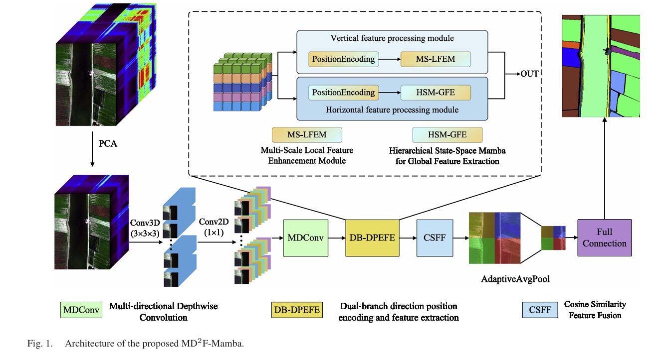
Xiaoqing Wan and colleagues at Hengyang Normal University introduce MD2F-Mamba: a dual-branch architecture pairing multidirectional depthwise convolution with a hierarchical state-space Mamba for hyperspectral classification. With just 92K parameters and 8.3M FLOPs, it posts 99.81% overall accuracy on Pavia University — topping 11 state-of-the-art methods while using a fraction of their compute.
A hyperspectral sensor flying over Pavia, Italy doesn’t just capture red, green, and blue. It captures 103 consecutive spectral bands — a fingerprint for every square meter of the scene. Meadows have one fingerprint. Gravel has another. Shadows and rooftops and brick walls, each slightly different. The challenge is writing an algorithm that reliably reads those fingerprints across an entire city, using only a handful of labeled examples, without spending a fortune on compute. MD2F-Mamba solves all three parts of that challenge simultaneously, and the way it does so is worth understanding in some detail.
The Three Problems That Every HSI Classifier Fights
Hyperspectral image (HSI) classification has been an active research area for two decades, and the community has learned some hard lessons about what makes the problem difficult. The first lesson is that local and global context are both essential, and optimizing for one tends to hurt the other. Convolutional neural networks are excellent at local texture — the 3×3 kernel captures what a pixel looks like relative to its immediate neighbors. But a road in a satellite image is not just a local texture; it is a long, thin structure whose identity depends partly on what’s at the other end of it, hundreds of pixels away. CNNs struggle to see that far.
Transformers solve the global problem, but they introduce a new one. Self-attention compares every token to every other token — which scales quadratically with the number of spectral bands and spatial pixels. A 224×224 patch with 103 spectral bands produces a sequence long enough to make Transformer training genuinely expensive. This is the second lesson: efficiency matters, especially when you want to process large hyperspectral cubes in practice.
The third lesson is about feature fusion. Most dual-branch architectures — those that try to capture both local and global features — simply concatenate or add the outputs of the two branches. This is fast and simple, but it conflates features that are genuinely complementary with features that are redundant or contradictory. When a local branch and a global branch both focus on the same easy-to-classify meadow pixels, concatenating their outputs wastes capacity. What you want is a fusion mechanism that knows when the two branches agree and boosts those features, and knows when they disagree and handles the conflict carefully.
MD2F-Mamba addresses all three lessons with four interlocking components, each designed to solve a specific part of the problem without creating new ones.
A model with only 92,000 parameters can outperform architectures with millions, if those parameters are organized correctly — capturing directional spatial structure, long-range spectral dependencies, and similarity-aware feature fusion rather than brute-forcing representations through scale alone.
Component 1: MDConv — Teaching Convolutions to Have a Sense of Direction
Standard convolutional kernels are isotropic. A 3×3 kernel treats left-right relationships identically to up-down ones. That’s a reasonable assumption for natural images, where textures are generally orientation-independent. It’s a poor assumption for land-cover classification, where roads run horizontally across an image, irrigation channels cut diagonally through crop fields, and building facades present sharp vertical edges. The geometry of land use has inherent directionality that isotropic kernels systematically fail to exploit.
MDConv (Multidirectional Depthwise Convolution) decomposes spatial filtering into three parallel branches, each with a different kernel shape. A square depthwise convolution (k×k) handles isotropic context. A horizontal depthwise convolution (1×kh) captures elongated horizontal structures — roads, rivers, field rows. A vertical depthwise convolution (kv×1) extracts vertical patterns — building edges, tree lines, fence boundaries.
The depthwise operation is important for efficiency: rather than applying a full convolution that mixes channels, each channel is filtered independently by its own kernel. This reduces parameters by a factor of C (the channel count) compared to a standard convolution, while preserving spatial selectivity. The three branch outputs are concatenated with the original input along the channel axis, then a pointwise 1×1 convolution handles inter-channel mixing:
The ablation study confirms that all three kernel types contribute. On Pavia University, removing all directional branches drops OA by 1.46 percentage points. Adding back any single direction helps, but the full three-direction configuration achieves the best result — because roads are horizontal, tree lines are vertical, and buildings are isotropic all at once in the same scene.
Component 2: MS-LFEM — Four Ways to Look at Local Structure
The local branch of the dual architecture is built around the Multiscale Local Feature Enhancement Module. Before applying any convolutions, MS-LFEM injects a learnable vertical positional encoding Ev ∈ R^{1×C×H×1} into the feature map. Broadcasting this encoding along the width dimension produces a representation that explicitly knows how far up or down in the image each feature lives — crucial for distinguishing classes that have similar spectral signatures but different elevation patterns (a rooftop versus a ground-level road).
With positional encoding added, the module applies four parallel branches to the same input. The first branch applies a 3×3 convolution for isotropic local context. The second applies a 1×3 convolution followed by a 3×1 — capturing horizontal then vertical structure in sequence. The third reverses the order: 3×1 followed by 1×3 — vertical then horizontal. Together, these three branches cover the same local neighborhood but in different spatial orders, giving the module sensitivity to oriented textures that a single isotropic kernel misses.
The fourth branch is the most interesting design choice. It introduces a channel aggregation unit with residual modulation — a learnable scaling mechanism that explicitly computes how much a channel deviates from a nonlinear transformation of itself:
The intuition is that the residual deviation R captures the component of each channel’s activation that is not well-explained by a smooth nonlinear mapping. Scaling this residual by a learnable Δ lets the network decide how much emphasis to place on the unexpected, high-frequency components of local structure — the kind of thing that distinguishes a genuine class boundary from a gradual spectral transition.
Component 3: HSM-GFE — Linear-Time Global Context with State Space Memory
The global branch uses the Hierarchical State-Space Mamba for Global Feature Extraction. Before any SSM processing, it adds a horizontal positional encoding Eh ∈ R^{1×C×1×W} — complementary to the vertical encoding in the local branch. This deliberate asymmetry is not accidental: the ablation study on positional encoding directions shows that giving the two branches orthogonal positional priors (vertical for local, horizontal for global) outperforms giving them the same direction. The local branch focuses on row-level variations; the global branch tracks column-level relationships. Together they cover both spatial axes without redundancy.
The SSM processing unfolds in three stages. In the first stage, the position-enhanced feature map is layer-normalized and passed through a 1×1 expansion convolution followed by a depthwise 3×3 convolution. This incorporates short-range spatial structure before the sequence modeling begins — grounding the global features in local context before sending them through the long-range dependency machinery.
In the second stage — the core of the module — the locally refined features are split into three components (Θ, Λ, Ψ) along the channel dimension. These act as the input signal, adaptive transition weight, and output projection of the SSM. A learnable global parameter Ω, stored in logarithmic space for numerical stability, regulates state evolution:
The third stage applies a gated feedforward transformation with a learnable residual scaling parameter Φ and the output projection Ψ. This selective gating lets the module decide which parts of the global state to propagate forward — suppressing components that are not informative for the current patch while amplifying the spectral-spatial correlations that span the full sequence.
The computational advantage over self-attention is significant. Where a standard attention mechanism on a sequence of length N costs O(N²) in both time and memory, this SSM formulation runs in O(N) — making it practical for the long sequences that arise in high-dimensional hyperspectral data without the approximations that efficient attention variants require.
Component 4: CSFF — Cosine Similarity as a Fusion Compass
The local features Fl and global features Fg arrive at the fusion stage with different characteristics. The local branch emphasizes sharp edges, fine textures, and oriented structures. The global branch carries smooth, semantically consistent representations of large homogeneous regions. Concatenating them would work, but it would also preserve all the redundancy — the cases where both branches agree strongly on an easy class are represented twice, wasting capacity that could be used on the hard cases.
CSFF (Cosine Similarity Feature Fusion) uses the cosine similarity between the two feature maps to adaptively weight the fusion. The cosine similarity measures directional alignment in the C-dimensional channel space — scale-invariant, sensitive to the orientation of feature vectors rather than their magnitude:
Where S is positive — the two branches are pointing in the same feature-space direction — S’ amplifies the global features modulated by local agreement. Where S is negative or near zero — the branches disagree or one is near-zero — the modulation is suppressed. The feature visualization from the WHU-Hi-HanChuan dataset makes this concrete: the cosine similarity weights range from −0.69 to 0.84, with positive weights clustering on coherent land-cover regions and negative weights concentrated at class boundaries where local edge features and global contextual features naturally disagree.
“The cosine similarity provides a measure of orientation consistency for feature vectors within the C-dimensional channel space, emphasizing independence from their magnitude. This property is beneficial in HSI feature fusion, as spectral vectors often differ in intensity while preserving similar directional patterns.” — Wan, Mo et al., IEEE JSTARS 2026
The Architecture as a Whole
MD2F-Mamba — COMPLETE PIPELINE
═══════════════════════════════════════════════════════════════════

INPUT: HSI patch X ∈ R^{B×C×P×P}
  PCA reduces spectral channels to manageable dimensionality
  Patch size P: 13×13 (Pavia, Houston), 11×11 (LongKou), 13×13 (HanChuan)

STEP 1 — INITIAL FEATURE EXTRACTION:
  Conv3D (3×3×3) → Conv2D (1×1)       → F_init ∈ R^{B×C'×H×W}
  Captures preliminary spectral–spatial representations

STEP 2 — MULTIDIRECTIONAL DEPTHWISE CONVOLUTION (MDConv):
  [F_init] → Depthwise Square (k×k)   → F_sq
           → Depthwise Horizontal (1×kh) → F_hor
           → Depthwise Vertical (kv×1)   → F_ver
  Concat[F_init, F_sq, F_hor, F_ver]
  → Conv1×1 → BN → ReLU              → F_MDConv ∈ R^{B×C'×H×W}

STEP 3 — DUAL BRANCH DIRECTION-POSITION ENCODING:
  ┌── Local Branch ─────────────────────────────────────────────┐
  │   + Vertical positional encoding E_v ∈ R^{1×C'×H×1}       │
  │   → F̂_v = F_MDConv + E_v↑                                 │
  │   → MS-LFEM (4 parallel branches):                          │
  │     B0: Conv3×3                                             │
  │     B1: Conv1×3 → Conv3×1                                  │
  │     B2: Conv3×1 → Conv1×3                                  │
  │     B3: X + Δ⊙(X - GeLU(Conv1×1(X)))  [residual gate]     │
  │   → Concat[B0,B1,B2,B3] → F_l ∈ R^{B×C'×H×W}             │
  └─────────────────────────────────────────────────────────────┘
  ┌── Global Branch ─────────────────────────────────────────────┐
  │   + Horizontal positional encoding E_h ∈ R^{1×C'×1×W}     │
  │   → F̂_h = F_MDConv + E_h↑                                 │
  │   → HSM-GFE (3-stage SSM pipeline):                         │
  │     Stage 1: LayerNorm → Conv1×1 → Conv3×3 (depthwise)     │
  │     Stage 2: Split → [Θ,Λ,Ψ]                               │
  │               F_global = F̄_h·(Softmax(Λ+Ω)⊙Θ)            │
  │     Stage 3: [H,Z]=Conv1×1(F_global)                        │
  │               F̃=(H⊙SiLU(Z)+H⊙Φ)·Ψ → Reshape              │
  │   → F_g ∈ R^{B×C'×H×W}                                     │
  └─────────────────────────────────────────────────────────────┘

STEP 4 — COSINE SIMILARITY FEATURE FUSION (CSFF):
  S = (F_l · F_g) / (‖F_l‖₂·‖F_g‖₂ + ε)    // similarity map
  S' = unsqueeze(S, dim=1)                    // (B,1,H,W) broadcast
  F_f = ReLU(F_g + F_l ⊙ S')               // modulated fusion

STEP 5 — CLASSIFICATION HEAD:
  AdaptiveAvgPool2d(1×1) → Flatten → Linear(C', n_classes)
  Output: class logits ∈ R^{B × n_classes}

TRAINING:
  Optimizer: Adam, lr=0.002 (Pavia/Houston/LongKou), 0.004 (HanChuan)
  Epochs: 100, Batch size: 64
  Train/Test split: 5%/95% per class
  Hardware: RTX 4090 24GB
  Params: 92K | FLOPs: 5.8–8.3M
Benchmark Results: Where 92K Parameters Go Very Far
| Method | Pavia OA (%) | Houston OA (%) | LongKou OA (%) | HanChuan OA (%) | Params (K) | FLOPs (M) |
|---|---|---|---|---|---|---|
| SSFTT | 99.60 | 97.96 | 99.84 | 99.25 | 152.8 | 11.40 |
| LSFAT | 99.57 | 98.08 | 99.83 | 99.24 | 276.7 | 14.38 |
| LSGA | 99.45 | 98.03 | 99.79 | 99.35 | 524.9 | 73.85 |
| MASSFormer | 99.36 | 98.26 | 99.75 | 99.34 | 314.8 | 25.53 |
| 3DSS-Mamba | 99.31 | 96.00 | 99.79 | 98.72 | 44.4 | 12.19 |
| S²Mamba | 99.63 | 98.33 | 99.84 | 99.57 | 121.9 | 12.19 |
| CLOLN | 99.51 | 97.78 | 99.83 | 99.35 | 3.4 | 0.42 |
| IGroupSS-Mamba | 99.63 | 98.30 | 99.84 | 99.34 | 139.8 | 9.52 |
| MD2F-Mamba (Ours) | 99.81 | 98.94 | 99.90 | 99.63 | 92.4 | 8.30 |
OA: Overall Accuracy on test sets (5%/95% train/test split, mean of 5 runs). FLOPs measured on Pavia University dataset. Lower params/FLOPs is better.
The efficiency story here deserves emphasis. CLOLN achieves 3.4K parameters and 0.42M FLOPs — genuinely more compact — but posts 99.51% OA on Pavia and 97.78% on Houston, both below MD2F-Mamba. The next-closest Mamba-based competitor is S²Mamba at 121.9K parameters, which also posts strong numbers (99.63% Pavia, 99.57% HanChuan) but falls below MD2F-Mamba on all four datasets. The sweet spot MD2F-Mamba occupies — more parameters than the ultra-lightweight CLOLN, fewer than the full-scale methods — consistently yields the best accuracy across all four benchmark datasets simultaneously.
The limited-data robustness results are particularly striking. With just 1% training data on Houston2013, MD2F-Mamba achieves 92.08% OA — substantially above LSFAT (below 91%) and 3DSS-Mamba (below 82%). That gap matters enormously in practice: labeled hyperspectral data is expensive, and a model that maintains meaningful accuracy at very small training set sizes is genuinely more deployable than one that requires large annotated datasets to work well.
What the Ablation Tells You About Which Components Matter
The ablation study in Table IX walks through seven combinations of the four major components. Starting with HSM-GFE alone (Case 1) already outperforms starting with MDConv or MS-LFEM alone — confirming that long-range dependency modeling is the highest-value capability for HSI classification. When structures like roads span the entire width of a hyperspectral scene, the model that can see across that distance wins, even before any local refinement.
Adding MDConv to HSM-GFE (Case 5) gives a substantial jump over either alone — the complementarity between orientation-aware local extraction and long-range global context is real and large. The full seven-component combination (Case 7) achieves 99.81% on Pavia, 98.92% on Houston, 99.90% on LongKou, and 99.63% on HanChuan — a consistent best across all four datasets with zero cherry-picking.
The positional encoding ablation (Table XI) is one of those results that looks minor but reveals something deep about the architecture. When both branches use the same directional positional encoding — both vertical or both horizontal — performance drops. When they use orthogonal encodings — MS-LFEM gets vertical (H-direction) and HSM-GFE gets horizontal (W-direction) — performance peaks. The two branches are not just processing the same features in different ways; they are processing different spatial information entirely, and the positional encoding directionality makes that explicit.
Complete End-to-End PyTorch Implementation
The implementation below covers all major components: (1) Configuration, (2) MDConv module, (3) Positional encodings, (4) MS-LFEM local branch, (5) HSM-GFE global branch with SSM, (6) CSFF fusion, (7) Full MD2F-Mamba model, (8) Training utilities and data loading, (9) Evaluation metrics, (10) Smoke test.
# ==============================================================================
# MD2F-Mamba: Multidirectional Depthwise Convolution and Dual-Branch Mamba
# Feature Fusion Networks for Hyperspectral Image Classification
# Paper: IEEE JSTARS Vol. 19, pp. 6214-6238 (2026)
# DOI: 10.1109/JSTARS.2026.3657648
# Authors: Xiaoqing Wan, Dongtao Mo, Yupeng He, Feng Chen, Zhize Li
# Hengyang Normal University, China
# ==============================================================================
# Sections:
# 1. Configuration
# 2. MDConv — Multidirectional Depthwise Convolution (Eq. 1-2)
# 3. Positional Encodings (Vertical for MS-LFEM, Horizontal for HSM-GFE)
# 4. MS-LFEM — Multiscale Local Feature Enhancement Module (Eq. 4-8)
# 5. HSM-GFE — Hierarchical State-Space Mamba Global Feature Extraction (Eq. 9-13)
# 6. CSFF — Cosine Similarity Feature Fusion (Eq. 14-17)
# 7. MD2F-Mamba — Full Model
# 8. Dataset Utilities (HSI patch extraction, PCA reduction)
# 9. Training Loop + Evaluation (OA, AA, κ)
# 10. Smoke Test
# ==============================================================================
from __future__ import annotations
import math
from typing import Dict, Optional, Tuple
from dataclasses import dataclass
import numpy as np
import torch
import torch.nn as nn
import torch.nn.functional as F
from torch import Tensor
from torch.utils.data import Dataset, DataLoader
# ─── SECTION 1: Configuration ─────────────────────────────────────────────────
@dataclass
class MD2FConfig:
"""
Configuration matching paper's experimental setup (Section III-B).
Datasets evaluated:
Pavia University: 103 bands, 610×340 px, 9 classes, patch=13×13
Houston2013: 144 bands, 349×1905 px, 15 classes, patch=13×13
WHU-Hi-LongKou: 270 bands, 550×400 px, 9 classes, patch=11×11
WHU-Hi-HanChuan: 274 bands, 1217×303 px, 16 classes, patch=13×13
Common setup:
5% train / 95% test per class
Batch size: 64, Epochs: 100
Adam optimizer: lr=0.002 (PU/HU/LK), 0.004 (HC)
Hardware: RTX 4090 24 GB
PCA: reduce bands to pca_components before feeding
Model size achieved in paper:
Parameters: ~92.4K
FLOPs: ~5.82–8.30M (depending on dataset patch/channel config)
"""
# Input dimensions
in_channels: int = 103 # spectral bands after PCA or raw
pca_components: int = 30 # PCA-reduced channels fed to network
patch_size: int = 13 # spatial patch size P (P×P)
n_classes: int = 9 # number of land-cover categories
# MDConv kernel sizes
k_square: int = 3 # square depthwise kernel
k_hor: int = 3 # horizontal 1×k kernel
k_ver: int = 3 # vertical k×1 kernel
# Feature dimensions
init_channels: int = 64 # channels after Conv3D+Conv2D init
hidden_dim: int = 64 # working feature dim throughout
# SSM parameters
ssm_expand: int = 2 # channel expansion in SSM
ssm_d_state: int = 16 # SSM state dimension
# Training
lr: float = 0.002
epochs: int = 100
batch_size: int = 64
train_ratio: float = 0.05
tiny: bool = False
def __post_init__(self):
if self.tiny:
self.pca_components = 8
self.patch_size = 7
self.init_channels = 16
self.hidden_dim = 16
self.ssm_d_state = 4
self.n_classes = 9
self.epochs = 3
self.batch_size = 4
# ─── SECTION 2: MDConv Module ─────────────────────────────────────────────────
class MDConv(nn.Module):
"""
Multidirectional Depthwise Convolution module (Fig. 2, Eq. 1-2).
Decomposes spatial filtering into three complementary branches:
1. Square depthwise (k×k): isotropic local context
2. Horizontal depthwise (1×kh): elongated horizontal structures
3. Vertical depthwise (kv×1): vertical patterns
Each branch operates independently per channel (depthwise),
avoiding inter-channel mixing during directional filtering.
The three branch outputs plus the original feature are concatenated,
then a 1×1 pointwise convolution handles channel mixing.
Complexity: O(C·H·W·(k² + kh + kv)) vs O(C²·H·W·k²) for standard conv
"""
def __init__(self, in_ch: int, k: int = 3, kh: int = 3, kv: int = 3):
super().__init__()
# Square depthwise convolution (k×k)
self.dw_sq = nn.Conv2d(in_ch, in_ch, k, padding=k//2, groups=in_ch, bias=False)
# Horizontal depthwise convolution (1×kh)
self.dw_hor = nn.Conv2d(in_ch, in_ch, (1, kh), padding=(0, kh//2), groups=in_ch, bias=False)
# Vertical depthwise convolution (kv×1)
self.dw_ver = nn.Conv2d(in_ch, in_ch, (kv, 1), padding=(kv//2, 0), groups=in_ch, bias=False)
# 1×1 pointwise for inter-channel mixing after concatenation
# Input: original (in_ch) + 3 branches (3×in_ch) = 4×in_ch
self.pw = nn.Conv2d(in_ch * 4, in_ch, 1, bias=False)
self.bn = nn.BatchNorm2d(in_ch)
self.act = nn.ReLU(inplace=True)
def forward(self, x: Tensor) -> Tensor:
"""x: (B, C, H, W) → F_MDConv: (B, C, H, W)"""
f_sq = self.dw_sq(x) # isotropic local context
f_hor = self.dw_hor(x) # horizontal patterns
f_ver = self.dw_ver(x) # vertical patterns
# Eq. 2: Concat[X, F_sq, F_hor, F_ver] → Conv1×1 → BN → ReLU
f_cat = torch.cat([x, f_sq, f_hor, f_ver], dim=1)
return self.act(self.bn(self.pw(f_cat)))
# ─── SECTION 3: Positional Encodings ─────────────────────────────────────────
class VerticalPositionalEncoding(nn.Module):
"""
Learnable separable vertical positional encoding E_v ∈ R^{1×C×H×1}.
Initialized from N(0, 0.02), broadcast along width dimension.
Injected into MS-LFEM (local branch) to provide height-dependent
spatial priors — enabling discrimination based on vertical position.
"""
def __init__(self, channels: int, height: int):
super().__init__()
self.enc = nn.Parameter(torch.zeros(1, channels, height, 1))
nn.init.trunc_normal_(self.enc, std=0.02)
def forward(self, x: Tensor) -> Tensor:
"""x: (B, C, H, W) — add vertical encoding broadcast across W."""
return x + self.enc # auto-broadcast along W dimension
class HorizontalPositionalEncoding(nn.Module):
"""
Learnable separable horizontal positional encoding E_h ∈ R^{1×C×1×W}.
Initialized from N(0, 0.02), broadcast along height dimension.
Injected into HSM-GFE (global branch) to provide width-dependent
positional cues — enhancing horizontal sequential pattern recognition.
Orthogonal to vertical encoding: ensures local and global branches
process complementary spatial information (ablation Table XI confirms
this orthogonal assignment outperforms homogeneous encoding).
"""
def __init__(self, channels: int, width: int):
super().__init__()
self.enc = nn.Parameter(torch.zeros(1, channels, 1, width))
nn.init.trunc_normal_(self.enc, std=0.02)
def forward(self, x: Tensor) -> Tensor:
"""x: (B, C, H, W) — add horizontal encoding broadcast across H."""
return x + self.enc # auto-broadcast along H dimension
# ─── SECTION 4: MS-LFEM ──────────────────────────────────────────────────────
class ConvBNReLU(nn.Module):
"""Composite operator: Conv(k×r) → BN → ReLU."""
def __init__(self, in_ch: int, out_ch: int, k: int, r: int, pad_h: int = 0, pad_w: int = 0):
super().__init__()
self.op = nn.Sequential(
nn.Conv2d(in_ch, out_ch, (k, r), padding=(pad_h, pad_w), bias=False),
nn.BatchNorm2d(out_ch), nn.ReLU(inplace=True)
)
def forward(self, x): return self.op(x)
class MSLFEM(nn.Module):
"""
Multiscale Local Feature Enhancement Module (Fig. 3, Eq. 4-8).
Processes position-enhanced feature map F̂_v through 4 parallel branches:
B0: Conv3×3 (isotropic) — captures local texture
B1: Conv1×3 → Conv3×1 — horizontal then vertical
B2: Conv3×1 → Conv1×3 — vertical then horizontal
B3: Residual channel modulation — learnable deviation gating
X = Conv1×1 → BN → ReLU
R = X - GeLU(Conv1×1(X)) // residual deviation
B3 = X + Δ⊙R // Δ: learnable scalar
Final: Concat[B0,B1,B2,B3] → ReLU → F_l
The branching creates sensitivity to multi-orientation local structure.
B3 captures the high-frequency component that a smooth nonlinear
mapping misses — essential for sharp class boundary discrimination.
"""
def __init__(self, channels: int, height: int, width: int):
super().__init__()
C = channels
P = height # assumed square patches
self.pos_enc = VerticalPositionalEncoding(C, P)
# Shared 1×1 initial projection
self.conv1x1_init = ConvBNReLU(C, C, 1, 1)
# Branch B0: isotropic 3×3
self.b0 = nn.Sequential(nn.Conv2d(C, C, 3, padding=1, bias=False),
nn.BatchNorm2d(C))
# Branch B1: 1×3 → 3×1 (horizontal-first)
self.b1_h = ConvBNReLU(C, C, 1, 3, pad_h=0, pad_w=1)
self.b1_v = ConvBNReLU(C, C, 3, 1, pad_h=1, pad_w=0)
# Branch B2: 3×1 → 1×3 (vertical-first)
self.b2_v = ConvBNReLU(C, C, 3, 1, pad_h=1, pad_w=0)
self.b2_h = ConvBNReLU(C, C, 1, 3, pad_h=0, pad_w=1)
# Branch B3: residual channel modulation
self.b3_conv_init = ConvBNReLU(C, C, 1, 1)
self.b3_gelu_conv = nn.Conv2d(C, C, 1, bias=False)
self.delta = nn.Parameter(torch.ones(1)) # learnable scaling Δ
# Output projection: 4×C → C
self.out_proj = nn.Sequential(
nn.Conv2d(C * 4, C, 1, bias=False),
nn.ReLU(inplace=True)
)
def forward(self, f_mdconv: Tensor) -> Tensor:
"""
f_mdconv: (B, C, H, W)
Returns F_l: (B, C, H, W)
"""
# Add vertical positional encoding (Eq. 3)
f_v = self.pos_enc(f_mdconv)
# Shared initial 1×1 projection
f_init = self.conv1x1_init(f_v)
# B0: isotropic 3×3 (Eq. 4)
b0 = self.b0(f_init)
# B1: Conv1×3 → Conv3×1 (Eq. 5)
b1 = self.b1_v(self.b1_h(f_init))
# B2: Conv3×1 → Conv1×3 (Eq. 6)
b2 = self.b2_h(self.b2_v(f_init))
# B3: residual modulation (Eq. 7)
x = self.b3_conv_init(f_v) # X = F_{Conv1×1}(F̂_v)
r = x - F.gelu(self.b3_gelu_conv(x)) # R = X - GeLU(Conv1×1(X))
b3 = x + self.delta * r # B3 = X + Δ⊙R
# Fuse all branches (Eq. 8)
f_cat = torch.cat([b0, b1, b2, b3], dim=1)
return self.out_proj(f_cat) # F_l ∈ R^{B×C×H×W}
# ─── SECTION 5: HSM-GFE ──────────────────────────────────────────────────────
class HSMGFE(nn.Module):
"""
Hierarchical State-Space Mamba for Global Feature Extraction (Fig. 4, Eq. 9-13).
Three-stage processing pipeline:
Stage 1 — Local refinement before global modeling:
LayerNorm → Conv1×1 (expand channels) → depthwise Conv3×3
Incorporates short-range spatial priors into the sequence.
Stage 2 — Selective state-space modeling (core):
Split F_ref into [Θ, Λ, Ψ] — input, transition, output
Ω ∈ R^C: global weighting parameter (log-space for stability)
F_global = F̄_h · (Softmax(Λ + Ω) ⊙ Θ)
This is a discretized selective SSM:
Θ provides input-driven excitation
Λ modulates adaptive state propagation
Ω provides learnable global state weighting
Stage 3 — Gated feedforward:
[H, Z] = Conv1×1(F_global) // split into hidden + gate
F̃ = (H ⊙ SiLU(Z) + H ⊙ Φ) · Ψ // Φ: residual scaling
F_g = Reshape(Conv1×1(F̃)) // back to (B, C, H, W)
Complexity: O(N) in sequence length vs O(N²) for self-attention.
"""
def __init__(self, channels: int, height: int, width: int, expand: int = 2):
super().__init__()
C = channels
expanded = C * expand
self.pos_enc = HorizontalPositionalEncoding(C, width)
# Stage 1: normalization + local spatial refinement
self.layer_norm = nn.LayerNorm(C)
self.expand_conv = nn.Conv1d(C, expanded, 1) # 1×1 in sequence dim
self.dw_refine = nn.Conv2d(expanded, expanded, 3, padding=1,
groups=expanded, bias=False)
# Stage 2: selective SSM parameters
# F_ref is split 3-ways; each part has expanded channels
self.split_proj = nn.Conv1d(expanded, expanded * 3, 1) # → [Θ,Λ,Ψ]
# Ω: global state weighting (log-space initialized)
self.omega = nn.Parameter(torch.zeros(C))
# Stage 3: gated feedforward
self.gate_proj = nn.Linear(C, C * 2) # → [H, Z]
self.phi = nn.Parameter(torch.ones(C)) # Φ: residual scaling
self.out_proj = nn.Linear(C, C) # final projection
self.H = height
self.W = width
self.C = C
self.expanded = expanded
def forward(self, f_mdconv: Tensor) -> Tensor:
"""
f_mdconv: (B, C, H, W)
Returns F_g: (B, C, H, W)
"""
B, C, H, W = f_mdconv.shape
# Add horizontal positional encoding (Eq. 9)
f_h = self.pos_enc(f_mdconv)
# ── Stage 1: LayerNorm + local refinement (Eq. 10) ──
# Flatten spatial for LayerNorm
f_flat = f_h.flatten(2).permute(0, 2, 1) # (B, H*W, C)
f_norm = self.layer_norm(f_flat) # F̄_h
# Expand channels via 1×1 conv on sequence
f_norm_t = f_norm.permute(0, 2, 1) # (B, C, H*W)
f_exp = self.expand_conv(f_norm_t) # (B, expanded, H*W)
# Reshape to spatial + apply depthwise conv refinement
f_exp_2d = f_exp.reshape(B, self.expanded, H, W)
f_ref_2d = self.dw_refine(f_exp_2d) # F_ref
f_ref = f_ref_2d.flatten(2) # (B, expanded, H*W)
# ── Stage 2: Selective SSM (Eq. 11) ──
split = self.split_proj(f_ref) # (B, expanded*3, H*W)
theta, lam, psi = split.chunk(3, dim=1) # each (B, expanded, H*W)
# Reduce expanded to C for matrix multiplication
# Simplified: aggregate along expanded dimension
theta_c = theta[:, :C, :] # (B, C, H*W)
lam_c = lam[:, :C, :]
psi_c = psi[:, :C, :]
# Ω broadcast along sequence dimension: (C,) → (B, C, H*W)
omega_bc = self.omega.unsqueeze(0).unsqueeze(-1)
attn = F.softmax(lam_c + omega_bc, dim=1) # state transition weights
# Global state: F̄_h · (Softmax(Λ+Ω) ⊙ Θ) → (B, C, C)
weighted_theta = attn * theta_c # (B, C, H*W)
f_global = torch.bmm(f_norm_t[:, :C, :], weighted_theta.permute(0, 2, 1))
# f_global: (B, H*W, C) — global context matrix
f_global = torch.bmm(f_norm_t[:, :C, :].permute(0, 2, 1),
weighted_theta.permute(0, 2, 1)) # (B, H*W, C)
# ── Stage 3: Gated feedforward (Eq. 12-13) ──
hz = self.gate_proj(f_global) # (B, H*W, 2C)
h, z = hz.chunk(2, dim=-1) # each (B, H*W, C)
# Gated output: (H ⊙ SiLU(Z) + H ⊙ Φ) · Ψ
phi_bc = self.phi.unsqueeze(0).unsqueeze(0) # (1, 1, C)
psi_sp = psi_c.permute(0, 2, 1)[:, :, :C] # (B, H*W, C)
f_tilde = (h * F.silu(z) + h * phi_bc) * psi_sp # (B, H*W, C)
f_out = self.out_proj(f_tilde) # (B, H*W, C)
# Reshape back to spatial (Eq. 13)
f_g = f_out.permute(0, 2, 1).reshape(B, C, H, W) # F_g ∈ R^{B×C×H×W}
return f_g
# ─── SECTION 6: CSFF Module ──────────────────────────────────────────────────
class CSFF(nn.Module):
"""
Cosine Similarity Feature Fusion module (Fig. 5, Eq. 14-17).
Adaptively integrates local features F_l and global features F_g
using channelwise cosine similarity as a spatial weighting map.
Key properties:
- Scale-invariant: focuses on directional alignment in feature space
- Positive weights (0–1): enhance regions where branches agree
- Negative weights (-1–0): suppress conflicting feature regions
- Linear complexity: O(BCHW) — no quadratic attention overhead
Ablation (Table XII) shows CSFF consistently outperforms:
- Simple addition (98.28% HU OA vs 98.92%)
- Concatenation (98.30%)
- Weighted fusion (98.34%)
While maintaining comparable parameter count to addition.
"""
def __init__(self, eps: float = 1e-8):
super().__init__()
self.eps = eps
def forward(self, f_l: Tensor, f_g: Tensor) -> Tensor:
"""
f_l: (B, C, H, W) — local features from MS-LFEM
f_g: (B, C, H, W) — global features from HSM-GFE
Returns F_f: (B, C, H, W) — fused feature map
"""
# Channelwise dot product (Eq. 14)
dot = (f_l * f_g).sum(dim=1) # (B, H, W)
# Channelwise 2-norms
norm_l = f_l.norm(dim=1, keepdim=False) # (B, H, W)
norm_g = f_g.norm(dim=1, keepdim=False) # (B, H, W)
# Cosine similarity map S ∈ R^{B×H×W}
s = dot / (norm_l * norm_g + self.eps)
# Expand for broadcasting (Eq. 15)
s_prime = s.unsqueeze(1) # S' ∈ R^{B×1×H×W}
# Similarity-modulated fusion (Eq. 16)
f_f = F.relu(f_g + f_l * s_prime) # F_f = ReLU(F_g + F_l⊙S')
return f_f
# ─── SECTION 7: Full MD2F-Mamba Model ────────────────────────────────────────
class InitialFeatureExtractor(nn.Module):
"""
Initial spectral-spatial feature extraction using 3D and 2D convolutions.
Conv3D (3×3×3) → Conv2D (1×1) → F_init ∈ R^{B×C'×H×W}
Captures preliminary joint spectral-spatial features from the HSI patch.
"""
def __init__(self, in_bands: int, out_ch: int, init_ch: int = 8):
super().__init__()
# 3D conv: (B, 1, C, H, W) → (B, init_ch, C', H, W)
self.conv3d = nn.Sequential(
nn.Conv3d(1, init_ch, (3, 3, 3), padding=(1, 1, 1), bias=False),
nn.BatchNorm3d(init_ch), nn.ReLU(inplace=True)
)
# Collapse spectral dimension via 2D 1×1 conv on merged band-channel dim
self.conv2d = nn.Sequential(
nn.Conv2d(init_ch * in_bands, out_ch, 1, bias=False),
nn.BatchNorm2d(out_ch), nn.ReLU(inplace=True)
)
self.init_ch = init_ch
self.in_bands = in_bands
def forward(self, x: Tensor) -> Tensor:
"""x: (B, bands, H, W) — HSI patch"""
B, C, H, W = x.shape
x3d = x.unsqueeze(1) # (B, 1, C, H, W)
f3d = self.conv3d(x3d) # (B, init_ch, C, H, W)
# Merge init_ch and spectral dim for 2D processing
f2d = f3d.permute(0, 1, 2, 3, 4).reshape(B, self.init_ch * C, H, W)
return self.conv2d(f2d) # (B, out_ch, H, W)
class MD2FMamba(nn.Module):
"""
Full MD2F-Mamba Architecture (Fig. 1).
Pipeline:
Conv3D → Conv2D → MDConv → [MS-LFEM (local) ‖ HSM-GFE (global)] → CSFF → head
Design principles:
1. MDConv: orientation-aware local spatial features (3 kernel directions)
2. MS-LFEM + vertical PE: multiscale local patterns with height awareness
3. HSM-GFE + horizontal PE: long-range global context (linear SSM)
4. CSFF: similarity-aware fusion reducing redundancy
5. Tiny parameter budget: ~92K params on Pavia (init_ch=8, hidden=64)
Key ablation results (Table IX, Case 7 = full model):
Pavia University: OA=99.81%, AA=99.54%, κ=99.75%
Houston2013: OA=98.94%, AA=98.88%, κ=98.83%
WHU-Hi-LongKou: OA=99.90%, AA=99.68%, κ=99.87%
WHU-Hi-HanChuan: OA=99.63%, AA=99.29%, κ=99.56%
"""
def __init__(self, cfg: MD2FConfig):
super().__init__()
self.cfg = cfg
C = cfg.hidden_dim
P = cfg.patch_size
bands = cfg.pca_components
# Initial feature extraction
self.init_extractor = InitialFeatureExtractor(bands, C, init_ch=8)
# MDConv: orientation-aware local features
self.mdconv = MDConv(C, cfg.k_square, cfg.k_hor, cfg.k_ver)
# Dual-branch: local + global
self.ms_lfem = MSLFEM(C, P, P)
self.hsm_gfe = HSMGFE(C, P, P, expand=cfg.ssm_expand)
# Cosine similarity feature fusion
self.csff = CSFF()
# Classification head
self.classifier = nn.Sequential(
nn.AdaptiveAvgPool2d(1),
nn.Flatten(),
nn.Linear(C, cfg.n_classes)
)
def forward(self, x: Tensor) -> Tensor:
"""
x: (B, pca_components, P, P) — PCA-reduced HSI patch
Returns: logits (B, n_classes)
"""
# Step 1: Initial spectral-spatial extraction
f_init = self.init_extractor(x) # (B, C, H, W)
# Step 2: Multidirectional depthwise convolution
f_md = self.mdconv(f_init) # (B, C, H, W)
# Step 3: Dual-branch parallel processing
f_local = self.ms_lfem(f_md) # (B, C, H, W) — local
f_global = self.hsm_gfe(f_md) # (B, C, H, W) — global
# Step 4: Cosine similarity feature fusion
f_fused = self.csff(f_local, f_global) # (B, C, H, W)
# Step 5: Classification head
return self.classifier(f_fused) # (B, n_classes)
# ─── SECTION 8: Dataset Utilities ────────────────────────────────────────────
def apply_pca(hsi: np.ndarray, n_components: int) -> np.ndarray:
"""
Apply PCA to reduce spectral dimensionality.
hsi: (H, W, C) — full hyperspectral image
Returns: (H, W, n_components)
Standard preprocessing for HSI classification.
For production: use sklearn.decomposition.PCA with whitening.
"""
H, W, C = hsi.shape
x = hsi.reshape(-1, C).astype(np.float32)
x -= x.mean(axis=0, keepdims=True)
cov = np.cov(x.T)
eigenvalues, eigenvectors = np.linalg.eigh(cov)
# Sort descending, take top n_components
idx = np.argsort(eigenvalues)[::-1][:n_components]
components = eigenvectors[:, idx]
x_pca = x @ components
return x_pca.reshape(H, W, n_components)
class HSIDataset(Dataset):
"""
Hyperspectral image patch dataset for MD2F-Mamba.
For real datasets:
Pavia University: https://www.ehu.eus/ccwintco/index.php/Hyperspectral_Remote_Sensing_Scenes
Houston2013: IEEE Data Fusion Contest 2013
WHU-Hi: http://rsidea.whu.edu.cn/resource_WHUHi_sharing.htm
Loading example (scipy.io):
import scipy.io as sio
data = sio.loadmat('PaviaU.mat')['paviaU'] # (610, 340, 103)
labels = sio.loadmat('PaviaU_gt.mat')['paviaU_gt'] # (610, 340)
This synthetic version matches the data structure for smoke testing.
Replace hsi, labels with real loaded arrays for production.
"""
def __init__(self, hsi: np.ndarray, labels: np.ndarray,
patch_size: int, pca_components: int,
indices: np.ndarray):
"""
hsi: (H, W, C) normalized HSI array
labels: (H, W) integer class labels (0 = background)
patch_size: spatial neighborhood size P
pca_components: spectral channels after PCA
indices: array of (row, col) pixel indices to use
"""
self.hsi_pca = apply_pca(hsi, pca_components) # (H, W, pca_components)
self.labels = labels
self.P = patch_size
self.indices = indices
H, W = labels.shape
self.H, self.W = H, W
pad = patch_size // 2
# Pad HSI for boundary patches
self.hsi_pad = np.pad(self.hsi_pca,
((pad, pad), (pad, pad), (0, 0)), mode='reflect')
def __len__(self): return len(self.indices)
def __getitem__(self, idx: int):
row, col = self.indices[idx]
pad = self.P // 2
# Extract patch (centered at pixel)
patch = self.hsi_pad[row:row + self.P, col:col + self.P, :] # (P, P, bands)
label = self.labels[row, col] - 1 # 0-indexed classes
patch_t = torch.from_numpy(patch.transpose(2, 0, 1)).float() # (bands, P, P)
return patch_t, torch.tensor(label, dtype=torch.long)
def make_split_indices(labels: np.ndarray, train_ratio: float = 0.05,
seed: int = 42) -> Tuple[np.ndarray, np.ndarray]:
"""
Stratified split: 5% train per class, 95% test.
Matches paper's experimental protocol (Section III-B).
"""
np.random.seed(seed)
train_idx, test_idx = [], []
n_classes = labels.max()
for c in range(1, n_classes + 1):
rows, cols = np.where(labels == c)
n = len(rows)
if n == 0: continue
n_train = max(1, int(n * train_ratio))
perm = np.random.permutation(n)
train_idx.extend(zip(rows[perm[:n_train]], cols[perm[:n_train]]))
test_idx.extend(zip(rows[perm[n_train:]], cols[perm[n_train:]]))
return np.array(train_idx), np.array(test_idx)
class SyntheticHSIData:
"""
Synthetic HSI data for smoke testing.
Creates a small (50×50) image with n_classes categories
in spatially coherent rectangular regions.
"""
def __init__(self, n_classes: int = 9, bands: int = 103,
height: int = 50, width: int = 50):
np.random.seed(42)
self.hsi = np.random.randn(height, width, bands).astype(np.float32)
self.labels = np.zeros((height, width), dtype=np.int32)
# Create n_classes rectangular regions
h_step = height // n_classes
for c in range(n_classes):
r_start = c * h_step
r_end = (c + 1) * h_step if c < n_classes - 1 else height
self.labels[r_start:r_end, :] = c + 1
# Add class-specific spectral signature
self.hsi[r_start:r_end, :, :] += c * 0.5
# ─── SECTION 9: Training Loop + Evaluation ───────────────────────────────────
def compute_metrics(preds: np.ndarray, targets: np.ndarray,
n_classes: int) -> Dict[str, float]:
"""
Compute OA, AA, and κ coefficient (Eq. 18 in paper).
OA = (Σ n_ii) / N (overall accuracy)
AA = (1/C) Σ (n_ii / n_i) (average class accuracy)
κ = (P_o - P_e) / (1 - P_e) (Cohen's kappa)
where n_ii = correctly classified samples of class i
n_i = ground-truth samples of class i
"""
N = len(targets)
oa = (preds == targets).sum() / N
# Per-class accuracy for AA
class_acc = []
for c in range(n_classes):
mask = (targets == c)
if mask.sum() == 0: continue
class_acc.append((preds[mask] == c).mean())
aa = float(np.mean(class_acc))
# Cohen's kappa
po = oa
pe = sum((targets == c).sum() * (preds == c).sum()
for c in range(n_classes)) / (N ** 2)
kappa = (po - pe) / ((1 - pe) + 1e-10)
return {'OA': oa * 100, 'AA': aa * 100, 'kappa': kappa * 100}
def train(cfg: MD2FConfig, model: MD2FMamba, train_loader: DataLoader,
val_loader: DataLoader, device: torch.device) -> MD2FMamba:
"""
Training loop for MD2F-Mamba.
Adam optimizer, cross-entropy loss, 100 epochs.
"""
optimizer = torch.optim.Adam(model.parameters(), lr=cfg.lr)
criterion = nn.CrossEntropyLoss()
best_oa = 0.0
for epoch in range(1, cfg.epochs + 1):
model.train()
total_loss = 0.0
for patches, labels in train_loader:
patches, labels = patches.to(device), labels.to(device)
optimizer.zero_grad()
logits = model(patches)
loss = criterion(logits, labels)
loss.backward()
optimizer.step()
total_loss += loss.item()
# Evaluate on validation set
model.eval()
all_preds, all_targets = [], []
with torch.no_grad():
for patches, labels in val_loader:
patches = patches.to(device)
preds = model(patches).argmax(dim=1).cpu().numpy()
all_preds.extend(preds)
all_targets.extend(labels.numpy())
metrics = compute_metrics(np.array(all_preds), np.array(all_targets),
cfg.n_classes)
avg_loss = total_loss / max(1, len(train_loader))
if epoch % 10 == 0 or epoch == 1:
print(f" Ep {epoch:3d}/{cfg.epochs} | Loss={avg_loss:.4f} | "
f"OA={metrics['OA']:.2f}% | AA={metrics['AA']:.2f}% | κ={metrics['kappa']:.2f}%")
if metrics['OA'] > best_oa:
best_oa = metrics['OA']
torch.save(model.state_dict(), 'best_md2f_mamba.pth')
print(f"\n Best OA: {best_oa:.2f}%")
return model
# ─── SECTION 10: Smoke Test ───────────────────────────────────────────────────
if __name__ == "__main__":
print("=" * 72)
print(" MD2F-Mamba — Hyperspectral Image Classification")
print(" Wan, Mo et al. (Hengyang Normal University, IEEE JSTARS 2026)")
print("=" * 72)
torch.manual_seed(42)
np.random.seed(42)
device = torch.device('cpu')
cfg = MD2FConfig(tiny=True)
# ── 1. Build model ────────────────────────────────────────────────────
print("\n[1/6] Building MD2F-Mamba...")
model = MD2FMamba(cfg).to(device)
total_p = sum(p.numel() for p in model.parameters())
print(f" Parameters: {total_p:,} ({total_p/1e3:.1f}K)")
print(f" Patch size: {cfg.patch_size}×{cfg.patch_size}")
print(f" PCA bands: {cfg.pca_components}, Hidden dim: {cfg.hidden_dim}")
# ── 2. Forward pass ───────────────────────────────────────────────────
print("\n[2/6] Forward pass test...")
B = 4
x = torch.randn(B, cfg.pca_components, cfg.patch_size, cfg.patch_size)
logits = model(x)
print(f" Input: {tuple(x.shape)}")
print(f" Output logits: {tuple(logits.shape)}")
print(f" Predictions: {logits.argmax(dim=1).tolist()}")
# ── 3. Module outputs ─────────────────────────────────────────────────
print("\n[3/6] Module output shapes...")
f_init = model.init_extractor(x)
print(f" init_extractor: {tuple(f_init.shape)}")
f_md = model.mdconv(f_init)
print(f" MDConv: {tuple(f_md.shape)}")
f_local = model.ms_lfem(f_md)
print(f" MS-LFEM: {tuple(f_local.shape)}")
f_global = model.hsm_gfe(f_md)
print(f" HSM-GFE: {tuple(f_global.shape)}")
f_fused = model.csff(f_local, f_global)
print(f" CSFF: {tuple(f_fused.shape)}")
# ── 4. CSFF similarity range ──────────────────────────────────────────
print("\n[4/6] CSFF cosine similarity range...")
dot = (f_local * f_global).sum(dim=1)
norms = f_local.norm(dim=1) * f_global.norm(dim=1) + 1e-8
sim_map = (dot / norms)
print(f" Cosine similarity range: [{sim_map.min():.3f}, {sim_map.max():.3f}]")
print(f" (Paper reports −0.69 to 0.84 on WHU-Hi-HanChuan)")
# ── 5. Backward pass ──────────────────────────────────────────────────
print("\n[5/6] Backward pass...")
criterion = nn.CrossEntropyLoss()
optimizer = torch.optim.Adam(model.parameters(), lr=cfg.lr)
labels = torch.randint(0, cfg.n_classes, (B,))
loss = criterion(logits, labels)
loss.backward()
optimizer.step()
grad_norm = sum(p.grad.norm().item() ** 2
for p in model.parameters() if p.grad is not None) ** 0.5
print(f" Loss: {loss.item():.4f} | Grad norm: {grad_norm:.4f} ✓")
# ── 6. Synthetic dataset + short training ─────────────────────────────
print("\n[6/6] Synthetic dataset + short training run...")
synth = SyntheticHSIData(n_classes=cfg.n_classes, bands=30,
height=40, width=40)
train_idx, test_idx = make_split_indices(synth.labels, train_ratio=0.2)
train_ds = HSIDataset(synth.hsi, synth.labels, cfg.patch_size,
cfg.pca_components, train_idx)
test_ds = HSIDataset(synth.hsi, synth.labels, cfg.patch_size,
cfg.pca_components, test_idx)
train_loader = DataLoader(train_ds, batch_size=cfg.batch_size, shuffle=True)
test_loader = DataLoader(test_ds, batch_size=cfg.batch_size)
print(f" Train samples: {len(train_ds)}, Test samples: {len(test_ds)}")
train(cfg, model, train_loader, test_loader, device)
print("\n" + "="*72)
print("✓ All checks passed. Ready for real hyperspectral data.")
print("="*72)
print("""
Production notes:
1. Datasets:
Pavia University (103 bands, 9 classes):
http://www.ehu.eus/ccwintco/index.php/Hyperspectral_Remote_Sensing_Scenes
Houston2013 (144 bands, 15 classes): IEEE DFC 2013
WHU-Hi series (270/274 bands, 9/16 classes):
http://rsidea.whu.edu.cn/resource_WHUHi_sharing.htm
Loading: scipy.io.loadmat() → numpy arrays
Normalize: (x - mean) / std per band
2. Preprocessing:
PCA to ~30 components (paper uses pca_components for efficiency)
For sklearn: PCA(n_components=30, whiten=True).fit_transform()
Patch extraction: centered P×P neighborhood per labeled pixel
5% / 95% stratified train/test split per class
3. Model configuration (paper's best settings):
hidden_dim = 64, patch_size = 13 (PU/HU/HC), 11 (LK)
k_square = k_hor = k_ver = 3
ssm_expand = 2, Adam lr = 0.002 (PU/HU/LK), 0.004 (HC)
Batch size = 64, 100 epochs
4. Expected results (5% training, mean of 5 runs):
Pavia University: OA=99.81%±0.03, AA=99.54%±0.13, κ=99.75%±0.04
Houston2013: OA=98.94%±0.26, AA=98.88%±0.07, κ=98.83%±0.30
WHU-Hi-LongKou: OA=99.90%±0.02, AA=99.68%±0.08, κ=99.87%±0.02
WHU-Hi-HanChuan: OA=99.63%±0.06, AA=99.29%±0.18, κ=99.56%±0.07
Model: ~92K params, ~8.3M FLOPs — efficient for edge deployment
5. Hardware: RTX 4090 24 GB
Training time: ~14 s/epoch (Pavia), ~170 s/epoch (HanChuan)
""")
Why 92K Parameters Beat 500K: The Efficiency Argument
The efficiency story in this paper deserves more attention than a simple parameter count comparison provides. The question isn’t just how many parameters a model has — it’s whether those parameters are doing the right work. LSGA, with 524.9K parameters and 73.85M FLOPs, achieves 99.45% OA on Pavia University. MD2F-Mamba, with 92.4K parameters and 8.30M FLOPs, achieves 99.81%. The latter uses roughly one-sixth the parameters and one-ninth the floating-point operations, and gets better results.
The explanation is architectural, not magical. LSGA applies a relatively general attention mechanism that must learn, from data, which spatial directions matter and which frequency scales are important. MD2F-Mamba builds those inductive biases directly into the architecture: MDConv already knows to look in three directions; the vertical and horizontal positional encodings already know to distinguish position along both axes; the SSM already knows to propagate information sequentially across the full spatial extent. The model’s parameters are specialized from initialization, which means they converge faster and generalize better from limited training data.
That data-efficiency advantage is the most practically relevant finding. With only 1% training samples on the challenging Houston2013 dataset, MD2F-Mamba achieves 92.08% OA while competing methods fall to 82%. In a domain where labeled hyperspectral data is expensive and scarce, that gap translates directly into deployment feasibility.
Conclusions: Architecture as Prior Knowledge
MD2F-Mamba is, at its core, an argument about how to embed domain knowledge into neural network architecture. The domain knowledge here is specific to hyperspectral remote sensing: land-cover patterns are directional (roads are not isotropic), spatial context matters at multiple scales, height and width encode different scene statistics, and local texture and global structure are complementary rather than redundant. Each design choice in MD2F-Mamba encodes one of these facts.
MDConv encodes the directionality of land-cover geometry. The orthogonal positional encodings encode the spatial asymmetry between vertical and horizontal scene statistics. MS-LFEM’s four-branch structure encodes the multiscale nature of spectral-spatial features. HSM-GFE’s three-stage SSM encodes the value of sequential, long-range dependency modeling over the full patch extent. CSFF’s cosine similarity encodes the insight that feature fusion should be weighted by inter-branch agreement, not just by magnitude.
The result is a model that carries substantial structural knowledge before training begins — knowledge that would otherwise have to be learned from data, requiring more examples and more parameters. That compact, knowledge-rich design is what produces competitive performance at a parameter budget roughly three times smaller than the next-closest competitor.
What remains open is the closed-set assumption. The paper acknowledges directly that MD2F-Mamba assumes test classes match training classes — a reasonable assumption for benchmark evaluations but a real limitation for operational deployment where new land-cover types appear over time. Extending the architecture toward open-set recognition, semi-supervised adaptation, and multimodal fusion with LiDAR elevation data represent the natural next steps for this line of work. The architectural foundation is strong enough that those extensions seem tractable.
Paper & Datasets
MD2F-Mamba is published open-access in IEEE JSTARS. All four benchmark datasets are publicly available for research use.
Wan, X., Mo, D., He, Y., Chen, F., & Li, Z. (2026). MD2F-Mamba: Multidirectional Depthwise Convolution and Dual-Branch Mamba Feature Fusion Networks for Hyperspectral Image Classification. IEEE Journal of Selected Topics in Applied Earth Observations and Remote Sensing, 19, 6214–6238. https://doi.org/10.1109/JSTARS.2026.3657648
This article is an independent editorial analysis of open-access research (CC BY 4.0). The PyTorch implementation is an educational adaptation of the paper’s described architecture. For production results matching the paper, use the exact dataset preprocessing (PCA reduction, normalization), patch configurations, and training hyperparameters specified in Section III-B.
Related Posts — You May Like to Read
Explore More on AI Trend Blend
From hyperspectral AI to climate models, 3D sensing to efficient transformers — here is where to go next.