Key Points
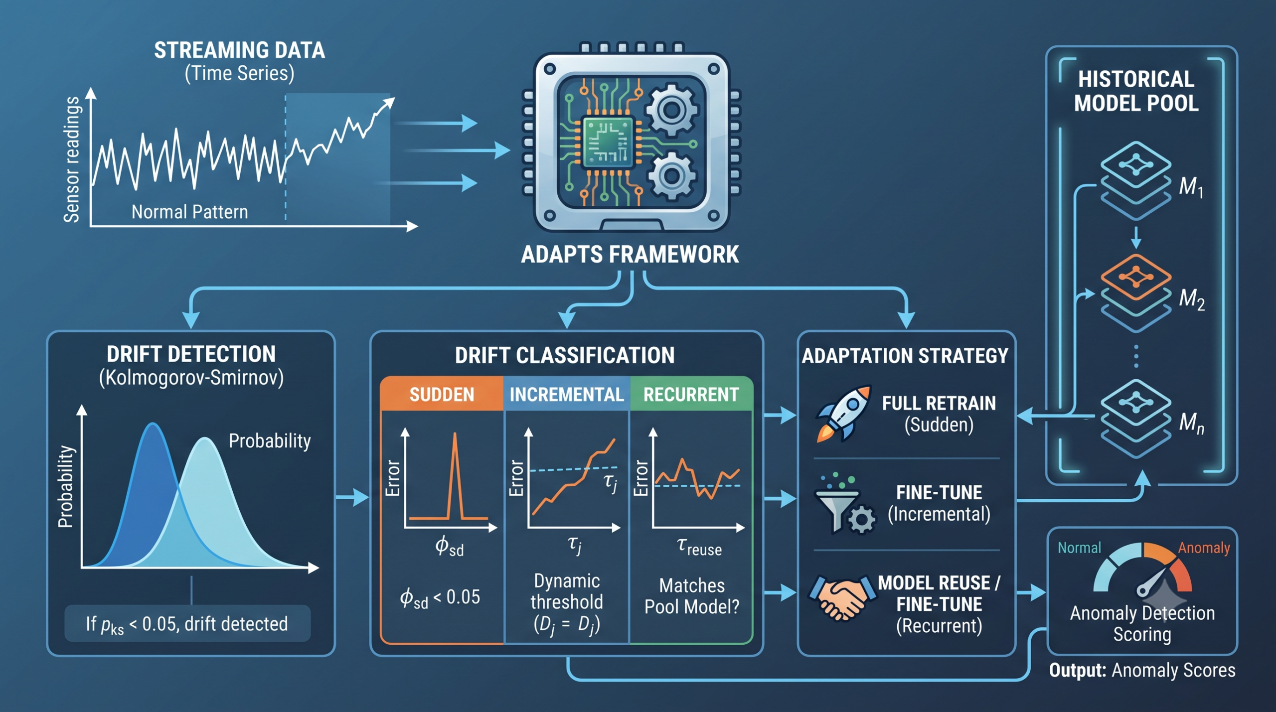
- ADAPTS is an unsupervised framework for anomaly detection in streaming time series that classifies concept drift as sudden, incremental, or recurrent before choosing how to adapt.
- A Kolmogorov-Smirnov test flags when a new window of data looks statistically different from the previous one, so the system only reacts when a real distributional change has occurred.
- Once drift is flagged, reconstruction error patterns decide the type. A sharp spike points to sudden drift, a rising trend points to incremental drift, and anything milder gets checked against a bounded pool of historical models for a possible match.
- Each drift type triggers a different response, full retraining for sudden drift, gentle fine tuning on a filtered subset for incremental drift, and direct reuse or fine tuning of a matched historical model for recurrent drift.
- Across six datasets ADAPTS posts the best average AUC, F1, and MCC among five baselines, though a repeated run analysis with ten random seeds shows its advantage disappears, and even reverses, on the dataset with the most tangled mix of drift types.
The Problem With One Update Strategy For Every Kind Of Change
Unsupervised anomaly detection on streaming data carries an unusual constraint baked into its name. There are no anomaly labels to learn from, only a continuous flow of mostly normal readings that a model has to characterize on its own. That job gets harder over time because the definition of normal rarely stays fixed. Human behavior shifts, seasons turn, equipment ages, and the boundary separating typical from anomalous readings moves along with all of it. This movement is concept drift, and left unaddressed it quietly degrades detection accuracy over months of continuous operation.
Concept drift does not arrive in one shape. A sudden drift changes the data distribution abruptly, the kind of shift you would see when a sensor fails or a system configuration changes overnight. An incremental drift accumulates slowly and consistently, the kind you would see as a component degrades or a season turns. A recurrent drift is really an old pattern coming back, a weekday traffic profile returning after a holiday, a summer temperature range showing up again a year later. Each of these calls for a different response. Sudden drift needs a model thrown out and replaced quickly. Incremental drift needs controlled, gradual adjustment. Recurrent drift needs a system that remembers what it already learned instead of relearning it from scratch.
Most existing approaches do not draw that distinction. Some assume the data stays stationary and never adapt at all. Others apply the same incremental update on every window regardless of what kind of change just occurred, which the authors point out creates two separate failure modes. Adaptation can lag behind a sudden shift because a small incremental nudge is not enough to catch up. Or the system can update unnecessarily during a mild, recurring fluctuation that did not need any change at all. A newer line of work, including STAD and Adaptive-LOF, adds a pool of historical models so old regimes can be reused instead of relearned. That is real progress, but these pool based methods still only ask whether a change happened, not what kind of change it was, and their historical model matching typically leans on a single similarity signal.
How ADAPTS Works
ADAPTS runs three modules in sequence for every new window of data, a distribution test that flags whether anything changed, a classifier that decides what kind of change it was, and an update mechanism that responds accordingly. The framework builds on an earlier system from the same University of Auckland group called AURORA, which introduced the bounded model pool and reuse mechanism but applied one unified update rule to every kind of drift. ADAPTS keeps the pool and adds the missing piece, explicit drift typing. You can read the full method and every table in the original paper, published open access in Knowledge-Based Systems.
Spotting Drift With A Statistical Test First
The first module answers a narrow question. Does the newest window of data look statistically different from the one before it. ADAPTS uses the two sample Kolmogorov-Smirnov test, comparing the empirical cumulative distribution functions of consecutive windows.
The resulting p value measures how likely both windows came from the same underlying distribution. When that p value drops below a guard threshold of 0.05, the standard cutoff in two sample hypothesis testing, ADAPTS declares drift and hands the window to the classification module.
If nothing crosses that threshold, the system keeps scoring anomalies with the model it already has, avoiding an update it does not need. That restraint matters more than it sounds. Every unnecessary retrain or fine tune is a chance to overwrite something the model already learned correctly.
Deciding Whether The Drift Is Sudden, Incremental, Or Recurrent
Once drift is confirmed, ADAPTS looks at how the previous model’s reconstruction error behaves on the new window. A Variational Autoencoder trained on normal patterns tends to reconstruct familiar data well and unfamiliar data poorly, so a jump in reconstruction error is itself a signal about what kind of change occurred.
For sudden drift, ADAPTS sets a dynamic threshold from the mean and standard deviation of the previous window’s reconstruction loss, following the three sigma convention used across statistical process monitoring.
If at least half the samples in the new window exceed that threshold, the drift is labeled sudden and the system prepares a full retrain.
Requiring a majority of samples, not just one or two outliers, is a deliberate filter. It keeps a handful of unusual points from triggering a full model replacement over what might just be ordinary anomalies. If the sudden drift condition is not met, ADAPTS checks the reconstruction error for a trend instead of a spike, fitting a regression slope across the window. A positive slope beyond a small threshold gets labeled incremental drift, matching the idea that this kind of change builds up gradually rather than jumping all at once.
Anything left over, meaning drift was detected but neither the sudden nor the incremental pattern showed up clearly, gets treated as a candidate for recurrent drift. That is a slightly unusual definition worth sitting with. Recurrent drift here is not defined by positively recognizing an old pattern up front. It is defined by elimination, a milder change that does not fit the other two categories, followed by a check against historical models to see whether it actually matches something the system has seen before.
Matching History Through A Two Stage Search
The candidate recurrent case does the most interesting work in the paper. ADAPTS keeps a bounded pool of historical models, each stored with the window it was trained on and how many times it has been reused. Searching the entire pool for every candidate window would be wasteful, so ADAPTS filters first and matches carefully second.
The filtering stage ranks every pooled model by a blend of two signals, how statistically similar its training window is to the current one using the same Kolmogorov-Smirnov test, and how often it has been reused historically, on the idea that a model reused often has proven itself reliable across past drift events.
The top ranked candidates move to a second, more expensive stage, where ADAPTS compares reconstruction error distributions using the Wasserstein distance between each candidate model’s historical performance and its performance on the current window.
Whichever candidate has the smallest distance becomes the selected model. If that distance falls below a reuse threshold, ADAPTS reuses the model directly with no further training. If it does not, the model is still judged the best available starting point, so ADAPTS fine tunes it rather than retraining from nothing. That is a subtle design choice worth noticing. Even when a historical model is not a close enough match to reuse outright, its parameters are treated as a useful head start rather than being discarded.
Four Ways To Update A Model
Once a drift type is settled, the update itself follows one of four fixed rules, retrain for sudden drift, fine tune for incremental drift, reuse or fine tune for recurrent drift, and a light touch fine tune when nothing has changed at all.
The filtered subset used for fine tuning deserves a mention. Rather than fine tuning on every point in the window, ADAPTS keeps only the central 50 percent of values, the inter quartile range, and discards the rest. That trims out exactly the points most likely to be anomalies or transient noise, which matters because fine tuning on contaminated data risks teaching the model that noise is normal.
What The Experiments Show
Six Datasets Covering Different Flavors Of Drift
The authors test ADAPTS on six time series collections chosen specifically because each one leans toward a different kind of drift. IoT sensor readings and the NAB benchmark contain frequent sudden and incremental shifts. The Yahoo anomaly benchmark leans heavily incremental. CEMACS ocean temperature readings and the University of Auckland’s own indoor air quality data show seasonal, recurrent patterns. A sixth dataset, called UoA-AirQuality-SE, is a deliberately stress tested variant built by concatenating busy and idle periods from the academic calendar without any transition between them, which forces sudden, incremental, and recurrent drift to overlap in the same stream.
Where ADAPTS Wins And By How Much
| Dataset | Dominant Drift | Best Baseline AUC | ADAPTS AUC |
|---|---|---|---|
| Yahoo | Incremental | AURORA, 0.88 | 0.88 (tie) |
| IoT | Sudden | AURORA, 0.94 | 0.96 |
| NAB | Sudden and Incremental | ECOD, 0.80 | 0.87 |
| CEMACS | Seasonal, Recurrent | AURORA, 0.91 | 0.91 (tie) |
| UoA-AirQuality | Seasonal, Recurrent | AURORA, 0.99 | 0.99 (tie) |
| UoA-AirQuality-SE | Mixed, Enforced Recurrent | AURORA, 0.96 | 0.92 |
Averaged across all six datasets, ADAPTS posts the best mean AUC at 0.92, ahead of AURORA’s 0.89 and well ahead of the remaining baselines. The gap is not evenly distributed. On IoT, dominated by sudden regime changes, ADAPTS reaches 0.96 AUC against AURORA’s 0.94, while the semi online method LODA and the static method ECOD trail badly at 0.62 and 0.26. On NAB, the dataset the authors highlight in their abstract, ADAPTS reaches 0.87 AUC, an 0.11 absolute gain over AURORA’s 0.76, which is the largest single jump in the whole comparison table. On the two seasonal, low volatility datasets, CEMACS and UoA-AirQuality, every competitive method performs similarly well, and ADAPTS’s edge narrows to a fraction of a point, since a stable, slowly cycling signal does not give an explicit drift classifier much extra to work with. On UoA-AirQuality-SE, the one dataset built to blend all three drift types together, AURORA actually posts the higher single run AUC.
Checking Whether The Gains Survive Ten Random Seeds
A single training run under one random seed can make any stochastic method look better or worse than it really is, and both AURORA and ADAPTS train a Variational Autoencoder, which means both carry some run to run variance. The authors rerun both frameworks under ten different random seeds and apply a paired Wilcoxon signed rank test to the resulting AUC scores.
| Dataset | AURORA AUC (10 seeds) | ADAPTS AUC (10 seeds) | Wilcoxon p Value |
|---|---|---|---|
| NAB | 0.78 ± 0.02 | 0.83 ± 0.019 | 0.004 (significant) |
| Yahoo | 0.85 ± 0.0079 | 0.87 ± 0.0095 | 0.002 (significant) |
| UoA-AirQuality | 0.98 ± 0.0027 | 0.99 ± 0.0022 | 0.010 (significant) |
| IoT | 0.87 ± 0.12 | 0.90 ± 0.043 | 0.846 (not significant) |
| CEMACS | 0.90 ± 0.0027 | 0.90 ± 0.0028 | 0.695 (not significant) |
| UoA-AirQuality-SE | 0.94 ± 0.01 | 0.90 ± 0.015 | 0.002 (significant, AURORA higher) |
The picture that emerges is more nuanced than the single run comparison suggests. On NAB, the AUC gain from 0.78 to 0.83 holds up as statistically significant. On Yahoo, a smaller gain from 0.85 to 0.87 is also significant. On UoA-AirQuality, ADAPTS’s tiny edge from 0.98 to 0.99 is likewise significant. On IoT and CEMACS the differences are not statistically significant, meaning the single run numbers in the headline comparison may partly reflect favorable variance rather than a guaranteed advantage.
Explicit drift typing helps most when a stream’s changes are cleanly separable, and can lose to a simpler unified strategy once several kinds of drift start to overlap in the same window. Reading of the repeated run findings in ADAPTS, University of Auckland
That reversal is worth sitting with rather than glossing over, because it amounts to the paper being candid about the limits of its own central idea. Classifying drift into three clean categories works well exactly when the underlying drift genuinely sorts into three clean categories. Once a stream is engineered, or simply happens, to blend an abrupt transition with a gradual trend and a repeating pattern all at once, forcing every window into one of three labels adds a decision that can go wrong, and a simpler pool based reuse strategy that does not try to be so specific turns out to be more robust in that particular setting.
What The Ablations And Sensitivity Tests Reveal
An ablation study tests what happens when individual pieces of ADAPTS are swapped out or unified. Removing drift detection entirely, so the model updates on every window regardless, drops F1 on Yahoo from 0.72 to 0.67. Swapping the Kolmogorov-Smirnov test for a Mann-Whitney U test knocks UoA-AirQuality-SE down from 0.83 to 0.78 F1, since that test reacts too eagerly to local fluctuations in a stream with sharp regime shifts. Forcing every detected drift through a single unified strategy tells a similar story. Full retraining on every detected drift is the worst option tested, dropping Yahoo’s F1 to 0.57, evidence that treating gradual change like an abrupt failure wastes the model’s accumulated knowledge for no benefit.
A unified pool based reuse strategy, interestingly, comes within half a point of the full framework on Yahoo, 0.71 against 0.72, and even edges past it on UoA-AirQuality-SE, 0.84 against 0.83, echoing the same lesson from the repeated run analysis. Historical model reuse alone gets you most of the way there, and full drift type classification adds a meaningful but modest amount stacked on top, except where drift types blur together, where it can occasionally cost a little instead.
A separate sensitivity sweep across window size, the incremental slope threshold, latent dimension, pool capacity, the top k candidate ratio, and the reuse threshold finds that almost none of these matter much within a reasonable range. The one exception is window size, and the reason is intuitive once stated. Yahoo’s dominant cycle runs 48 hours, and UoA-AirQuality-SE’s dominant cycle runs 24 hours. Setting the window size to match that cycle length gives ADAPTS a complete period to reason about in each step. Stretching the window to one and a half cycles instead drops Yahoo’s F1 from 0.72 to 0.64 and UoA-AirQuality-SE’s from 0.83 to 0.72. A framework built around detecting when a distribution changes needs its measurement window aligned with the data’s own rhythm, or it starts comparing partial cycles to each other and mistaking normal periodic variation for drift.
Where This Falls Short
The authors are unusually candid about scope in their own limitations section, and it is worth taking them at their word rather than smoothing it over. The Kolmogorov-Smirnov test at the center of Module 1 only compares one dimensional value distributions, which means the current framework is built for univariate streams, a single sensor or an aggregated signal, rather than multivariate data where several correlated variables drift together. The same test also only looks at marginal distributions, not temporal structure, so a stream whose values keep the same overall distribution but rearranges its temporal pattern could slip past undetected. The framework has not been tested on unstructured data such as images, text, or audio, and would need a different representation learning approach entirely to get there. The three way drift taxonomy, sudden, incremental, and recurrent, is also a simplification. Real streams can and do blend these patterns within the same window, and the UoA-AirQuality-SE results are a direct demonstration of what happens when they do. Finally, there is no benchmark dataset with ground truth drift type labels, so validating the accuracy of the classification step itself relies on visual inspection of a handful of example series rather than a quantitative score.
A Working Python Implementation
The code below implements the three ADAPTS modules as a working pipeline, a compact Variational Autoencoder, the Kolmogorov-Smirnov drift detector, the sudden and incremental classification rules, a bounded model pool with the two stage historical matching described above, and the four update strategies. A synthetic stream with an injected sudden jump and a slow incremental ramp exercises the full pipeline end to end. One implementation note on faithfulness. The paper selects the central 50 percent of samples in a window for fine tuning, but a Variational Autoencoder with a fixed input size cannot accept a shorter, filtered vector as a like for like replacement. This implementation clips extreme values toward the inter quartile bounds instead of dropping them outright, which keeps the window’s shape intact while still reducing the influence of outliers and transient noise, the same goal the paper describes for this step.
# adapts_pipeline.py
# Reference style implementation of the ADAPTS framework
# Li, Fan, Nair, and Wang, Knowledge-Based Systems 350 (2026) 116530

import numpy as np
import torch
import torch.nn as nn
import torch.optim as optim
from scipy.stats import ks_2samp, wasserstein_distance
from dataclasses import dataclass


class VAE(nn.Module):
    """Compact Variational Autoencoder matching the paper's setup,
    two hidden layers of 64 and 32 ReLU units on each side."""

    def __init__(self, window_size, latent_dim):
        super().__init__()
        self.enc1 = nn.Linear(window_size, 64)
        self.enc2 = nn.Linear(64, 32)
        self.mu = nn.Linear(32, latent_dim)
        self.logvar = nn.Linear(32, latent_dim)
        self.dec1 = nn.Linear(latent_dim, 32)
        self.dec2 = nn.Linear(32, 64)
        self.out = nn.Linear(64, window_size)

    def encode(self, x):
        h = torch.relu(self.enc1(x))
        h = torch.relu(self.enc2(h))
        return self.mu(h), self.logvar(h)

    def reparameterize(self, mu, logvar):
        std = torch.exp(0.5 * logvar)
        eps = torch.randn_like(std)
        return mu + eps * std

    def decode(self, z):
        h = torch.relu(self.dec1(z))
        h = torch.relu(self.dec2(h))
        return self.out(h)

    def forward(self, x):
        mu, logvar = self.encode(x)
        z = self.reparameterize(mu, logvar)
        recon = self.decode(z)
        return recon, mu, logvar


def vae_loss(recon, x, mu, logvar):
    # per-sample reconstruction error, used both for training and drift signals
    recon_err = ((recon - x) ** 2).mean(dim=1)
    kl = -0.5 * torch.sum(1 + logvar - mu.pow(2) - logvar.exp(), dim=1)
    return (recon_err + 0.01 * kl).mean(), recon_err.detach().numpy()


def train_vae(data, latent_dim, epochs=80, lr=1e-2):
    model = VAE(window_size=data.shape[1], latent_dim=latent_dim)
    opt = optim.Adam(model.parameters(), lr=lr)
    x = torch.tensor(data, dtype=torch.float32)
    for _ in range(epochs):
        opt.zero_grad()
        recon, mu, logvar = model(x)
        loss, _ = vae_loss(recon, x, mu, logvar)
        loss.backward()
        opt.step()
    return model


def finetune_vae(model, data, epochs=10, lr=1e-3):
    opt = optim.Adam(model.parameters(), lr=lr)
    x = torch.tensor(data, dtype=torch.float32)
    for _ in range(epochs):
        opt.zero_grad()
        recon, mu, logvar = model(x)
        loss, _ = vae_loss(recon, x, mu, logvar)
        loss.backward()
        opt.step()
    return model


def reconstruction_errors(model, data):
    x = torch.tensor(data, dtype=torch.float32)
    with torch.no_grad():
        recon, mu, logvar = model(x)
        _, errors = vae_loss(recon, x, mu, logvar)
    return errors


def select_iqr_subset(window):
    # Clip toward the central 50 percent (inter-quartile) range of values.
    # The paper selects the central 50 percent of samples for fine-tuning.
    # Dropping values outright would shrink the window below the VAE's
    # fixed input size, so this implementation clips extreme values toward
    # the IQR bounds instead, which preserves the window shape while still
    # reducing the influence of outliers and transient noise on fine-tuning.
    q1, q3 = np.percentile(window, [25, 75])
    return np.clip(window, q1, q3)


def ks_drift_detected(prev_window, curr_window, alpha=0.05):
    _, p_value = ks_2samp(prev_window.flatten(), curr_window.flatten())
    return p_value < alpha, p_value


def classify_drift(errors_prev, errors_curr, phi_sd=3.0, epsilon=0.0):
    tau = errors_prev.mean() + phi_sd * errors_prev.std()
    p_sd = (errors_curr > tau).mean()
    if p_sd >= 0.5:
        return "Sudden"
    slope = np.polyfit(np.arange(len(errors_curr)), errors_curr, 1)[0]
    if slope > epsilon:
        return "Incremental"
    return "Recurrent_Candidate"


@dataclass
class PoolEntry:
    model: VAE
    window: np.ndarray
    usage_count: int = 0


class ModelPool:
    def __init__(self, capacity=20):
        self.capacity = capacity
        self.entries = []

    def add(self, model, window):
        entry = PoolEntry(model=model, window=window, usage_count=0)
        if len(self.entries) < self.capacity:
            self.entries.append(entry)
        else:
            min_usage = min(e.usage_count for e in self.entries)
            for i, e in enumerate(self.entries):
                if e.usage_count == min_usage:
                    self.entries[i] = entry
                    break

    def select_topk(self, curr_window, k):
        usage = np.array([e.usage_count for e in self.entries], dtype=float)
        rng = usage.max() - usage.min()
        usage_norm = (usage - usage.min()) / rng if rng > 0 else np.zeros_like(usage)

        scored = []
        for e, u in zip(self.entries, usage_norm):
            _, sim_score = ks_2samp(curr_window.flatten(), e.window.flatten())
            rank_score = 0.5 * sim_score + 0.5 * u
            scored.append((rank_score, e))
        scored.sort(key=lambda t: t[0], reverse=True)
        return [e for _, e in scored[:k]]

    def best_match(self, curr_window, candidates):
        best_entry, best_dist = None, np.inf
        for e in candidates:
            curr_errors = reconstruction_errors(e.model, curr_window)
            hist_errors = reconstruction_errors(e.model, e.window)
            dist = wasserstein_distance(curr_errors, hist_errors)
            if dist < best_dist:
                best_dist, best_entry = dist, e
        return best_entry, best_dist


class ADAPTSStream:
    def __init__(self, window_size, latent_dim=2, pool_cap=20, top_k=3, tau_reuse=0.3):
        self.window_size = window_size
        self.latent_dim = latent_dim
        self.top_k = top_k
        self.tau_reuse = tau_reuse
        self.pool = ModelPool(capacity=pool_cap)
        self.current_model = None
        self.prev_window = None
        self.prev_errors = None

    def init_model(self, initial_data):
        self.current_model = train_vae(initial_data, self.latent_dim)
        self.pool.add(self.current_model, initial_data)
        self.prev_window = initial_data
        self.prev_errors = reconstruction_errors(self.current_model, initial_data)

    def process_window(self, window):
        drift, p_value = ks_drift_detected(self.prev_window, window)

        if not drift:
            label = "Normal"
            self.current_model = finetune_vae(self.current_model, select_iqr_subset(window), epochs=2)
        else:
            curr_errors = reconstruction_errors(self.current_model, window)
            label = classify_drift(self.prev_errors, curr_errors)

            if label == "Sudden":
                self.current_model = train_vae(window, self.latent_dim)
                self.pool.add(self.current_model, window)
            elif label == "Incremental":
                self.current_model = finetune_vae(self.current_model, select_iqr_subset(window))
                self.pool.add(self.current_model, window)
            else:
                candidates = self.pool.select_topk(window, self.top_k)
                best_entry, best_dist = self.pool.best_match(window, candidates)
                if best_dist < self.tau_reuse:
                    self.current_model = best_entry.model
                    best_entry.usage_count += 1
                    label = "Recurrent (reused)"
                else:
                    self.current_model = finetune_vae(best_entry.model, select_iqr_subset(window))
                    self.pool.add(self.current_model, window)
                    label = "Recurrent (fine-tuned)"

        self.prev_window = window
        self.prev_errors = reconstruction_errors(self.current_model, window)
        return label, p_value


if __name__ == "__main__":
    np.random.seed(0)
    torch.manual_seed(0)

    # Build a synthetic stream: stable sine wave, a sudden jump midway,
    # then a slow incremental ramp toward the end
    window_size = 32
    n_windows = 10
    stream = []
    for j in range(n_windows):
        t = np.linspace(0, 2 * np.pi, window_size)
        base = np.sin(t) + np.random.normal(0, 0.05, window_size)
        if j >= 4:
            base = base + 3.0  # sudden jump from window 4 onward
        if j >= 7:
            base = base + 0.3 * (j - 6)  # incremental ramp on top
        stream.append(base.reshape(1, -1))

    pipeline = ADAPTSStream(window_size=window_size)
    pipeline.init_model(stream[0])

    print("Running ADAPTS smoke test on a synthetic stream")
    for j in range(1, n_windows):
        label, p_value = pipeline.process_window(stream[j])
        print(f"window {j} drift_label={label} ks_p_value={p_value:.4f} pool_size={len(pipeline.pool.entries)}")

    print("Smoke test passed. Drift labels and pool size look consistent with the injected pattern.")
Where ADAPTS Ends Up
ADAPTS’s central achievement is teaching a streaming anomaly detector to ask two questions instead of one. Not just has something changed, but what kind of change is it, and the answer to that second question determines whether the system throws its old model away, nudges it gently, or reaches back into its own history for something that already fits. That distinction earns real gains on datasets where sudden, incremental, and recurrent drift show up in reasonably separable form, most visibly the 0.11 absolute AUC jump on NAB that survives a ten seed significance test.
The more interesting result, though, is the one the authors do not put in their abstract. On the dataset built specifically to blur the lines between drift types, the simpler predecessor framework AURORA beats ADAPTS by a statistically significant margin. Explicit drift classification is not a strategy that only ever helps. It is a strategy that helps when drift is separable and can cost you when it is not, because forcing an ambiguous change into one of three labels is itself a decision that can be wrong, while a system that just tries to reuse whatever fits best never has to make that call.
That finding generalizes past this one paper. Any system that adds interpretability by sorting messy reality into clean categories is making a bet that the categories actually fit the data it will see in deployment. For a factory sensor stream with a clear failure mode and a clear seasonal cycle, that bet pays off. For an environment where operating states blend into each other without a clean boundary, a framework that skips the categorization step and just asks which past experience looks closest may be the safer default, exactly what the unified pool reuse ablation shows coming within a fraction of a point of the full system.
None of this erases what ADAPTS demonstrates well. The window size finding, that aligning the measurement window with a stream’s natural cycle matters more than almost any other hyperparameter tested, is a genuinely transferable piece of practical advice for anyone building a drift detector on periodic data. The two stage historical model search, cheap statistical filtering followed by a more expensive distributional comparison on a small candidate set, is also a sensible pattern for keeping a growing model pool searchable without heavy compute. The open questions remain real too, this is a univariate framework tested on relatively short benchmark series, without a labeled drift type dataset to score the classification step directly.
Strip away the acronym, and ADAPTS is arguing something reasonably intuitive with genuine experimental honesty attached. Different kinds of change deserve different responses, most of the time, and the paper is willing to show you the one dataset where that idea runs into its own limits rather than hiding it in a footnote.
Frequently Asked Questions
What is ADAPTS designed to do
ADAPTS is an unsupervised framework for anomaly detection in streaming time series. It detects concept drift with a statistical test, classifies the drift as sudden, incremental, or recurrent, and applies a matching update strategy while keeping a bounded pool of historical models for reuse.
How does ADAPTS tell sudden drift apart from incremental drift
It looks at the previous model’s reconstruction error on the new window. A sharp spike above a dynamic threshold, set from the mean and standard deviation of recent error, gets labeled sudden. A gradual upward trend across the window gets labeled incremental instead.
What happens when drift does not look sudden or incremental
ADAPTS treats it as a candidate recurrent drift and checks it against a pool of historical models using a two stage search, first filtering by statistical similarity and reuse history, then comparing reconstruction error distributions with the Wasserstein distance. A close enough match gets reused directly, otherwise the closest match is fine tuned.
Does explicit drift classification always outperform a simpler strategy
No. A repeated run analysis with ten random seeds shows ADAPTS significantly outperforms its simpler predecessor AURORA on datasets like NAB and Yahoo, but AURORA significantly outperforms ADAPTS on a dataset engineered to blend sudden, incremental, and recurrent drift together in the same stream.
What are the main limitations of ADAPTS
The drift detection test only compares one dimensional value distributions, so the framework is built for univariate time series rather than multivariate data. It does not capture temporal structure directly, has not been tested on images, text, or audio, and there is no benchmark with ground truth drift type labels to score the classification step quantitatively.
Which datasets and baselines were used to test ADAPTS
The datasets are IoT sensor readings, the Yahoo anomaly benchmark, the Numenta Anomaly Benchmark, CEMACS ocean temperature data, and two University of Auckland indoor air quality datasets. The baselines are ECOD, LODA, STAD, Adaptive-LOF, and the authors’ own earlier framework, AURORA.
Read the full method, all six datasets, and every ablation table directly from the source.
This analysis is based on the published paper and an independent evaluation of its claims.