Key points
- The paper introduces an end to end graph neural network framework that forecasts and reconciles retail sales in one differentiable pipeline instead of two separate stages.
- Two model variants, TGLP-BUN and TALP-BUN, combine graph convolution or graph attention with gated recurrent units and a learnable nonlinear reconciliation head.
- The reconciliation step guarantees exact aggregation coherence by construction, because every upper level number is literally computed by summing the learned bottom level forecast.
- On a sparse Italian grocery hierarchy the gains concentrate above the item level, while on a denser Walmart hierarchy the gains spread across almost every level.
- Diebold Mariano tests, per node error distributions and multi step horizons all point the same direction, suggesting the improvement is broad rather than a lucky average.
The problem nobody solves by just forecasting harder
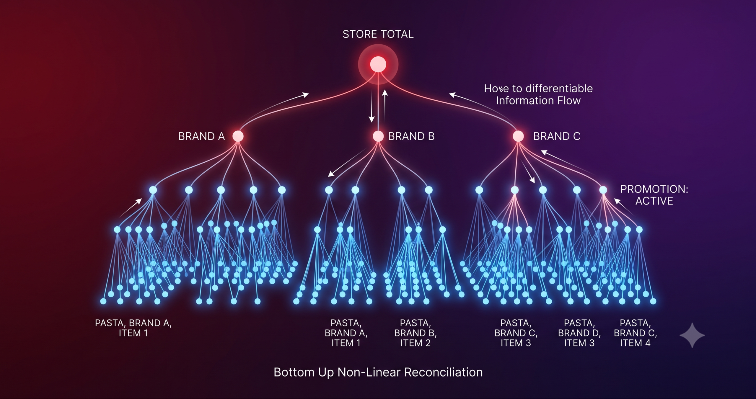
Retail demand planning would be simple if every product existed in isolation. It does not. A grocery chain needs a forecast for total daily revenue, for each brand it stocks, for each store, and for each item on the shelf, and every one of those numbers has to add up correctly. If the item level forecasts for a brand sum to more than the brand level forecast, someone in operations has to decide which number to believe, and that decision usually gets made by hand, under time pressure, using whichever number looks more familiar.
The formal name for this requirement is aggregation coherence. Forecasts at a parent node in the hierarchy must equal the sum of the forecasts at its children, at every point in time and at every forecast horizon. Classical statistics has known about this problem for decades. Bottom up forecasting solves it by only ever forecasting the smallest units and adding them up, which throws away whatever signal exists at the aggregate level. Top down forecasting solves it the other way, forecasting the total and splitting it using historical proportions, which throws away item specific behavior. A middle ground called optimal combination, most famously the MinT method from Wickramasuriya, Athanasopoulos and Hyndman, generates a forecast for every node and then reconciles them all at once using a linear correction built from the forecast error covariance matrix.
MinT works well enough that it remains one of the strongest baselines in the field, and the paper under discussion here uses it as a benchmark rather than dismissing it. But MinT is fundamentally a linear tool. Retail demand is not a linear system. Promotions create spikes that ripple unevenly across items. Some products sell every day, others sell in sparse, irregular bursts. A single linear correction matrix, however cleverly estimated, has to compromise across all of that heterogeneity at once.
Why the usual deep learning fix is only half a fix
Machine learning researchers noticed the same limitation and mostly responded in one of two ways. The first camp built better base forecasters, using tree based models or recurrent networks, and then bolted a classical reconciliation step on afterward, which is really just a fancier version of the same two stage pipeline. The second camp built fully end to end architectures that try to encourage coherence through the loss function or the network architecture itself, without an explicit reconciliation operator. Methods in this second group include SHARQ from Han, Dasgupta and Ghosh, HiReD from Paria and colleagues, PROFHIT, and HierE2E from Rangapuram and colleagues at Amazon.
The closest relative to the new paper is DeepHGNN, from Sriramulu, Fourrier and Bergmeir, which also combines graph message passing with temporal forecasting and enriches the hierarchy graph so information can flow across siblings and not just up and down parent child links. DeepHGNN encourages coherence with a joint loss over bottom level and aggregated forecasts, which is an implicit constraint rather than a guarantee. If the loss does not fully converge, or the network finds a shortcut, the coherence can slip.
The Auckland and Nanchang team argue that base forecasting and reconciliation are two different jobs and should stay two different modules, just not two different training stages. Their framework keeps the graph and temporal components focused purely on producing a base forecast for every node, and hands the coherence guarantee to a separate, explicit, differentiable reconciliation layer built directly on the summation matrix that defines the hierarchy. Because that layer is just an algebraic mapping from a learned bottom level vector to the full hierarchy through matrix multiplication, coherence is not something the network has to learn to respect. It is baked into the arithmetic.
Inside the architecture, module by module
The framework has three parts, all trained together in a single loss function rather than in separate stages. It helps to walk through each one the way you would walk through a factory line, because each stage hands something specific to the next.
Module one, treating the hierarchy as a graph
Every series in the hierarchy, whether it is the storewide total, a brand, or a single item, becomes a node in a graph. Edges connect parents to children, following the known structure of the retail hierarchy directly rather than inferring it from data. The authors also test similarity based graphs, built from cosine similarity between series, and a hybrid version that unions the two, though the main results in the paper use the pure hierarchy graph. At every time step, each node carries a small feature vector, typically the log transformed sales value and, when promotion data exists, a promotion indicator. For an aggregated node like a brand or a store, the promotion feature becomes a simple count of how many of its children are actively promoted that day, which is a neat way of letting promotion information climb the hierarchy without any manual feature engineering.
This graph and its node features get passed through either a graph convolutional network, following Kipf and Welling’s original formulation, or a graph attention network, following Velickovic and colleagues. The convolutional version treats every neighboring node with roughly equal weight when passing messages, while the attention version learns which neighbors matter more for a given node at a given moment. That distinction turns out to matter a great deal later in the results.
Module two, learning how each series moves through time
Once every node has a graph aware embedding at each time step, a shared gated recurrent unit processes the sequence for each node independently, updating a hidden state that summarizes the recent history of that series. A final linear layer turns that hidden state into a base forecast for the node. This is the point at which the model produces its first guess for every series in the hierarchy, and that guess is allowed to be incoherent. Nobody has told it yet that the brand total has to equal the sum of its items.
Module three, the reconciliation head that actually enforces the rule
This is the part that separates the paper from most of its competitors. The base forecasts for all nodes, coherent or not, get mapped down to a corrected bottom level vector through a learnable function, and the full hierarchy is then reconstructed by summing that corrected bottom level vector upward using the fixed summation matrix. The paper tests three versions of that mapping function, ranging from a simple selection of the existing bottom level forecasts, to a single learned linear correction, to a full multilayer perceptron with ReLU activations, layer normalization and dropout that can adjust each bottom level forecast nonlinearly based on the entire multi level forecast configuration. The strongest models in the paper, TGLP-BUN and TALP-BUN, both use this nonlinear version, referred to throughout as BUN.
The logic behind letting the correction be nonlinear and state dependent is worth sitting with for a moment, because it is the paper’s real conceptual contribution rather than just an engineering flourish. A linear correction assumes the adjustment needed at the bottom level is roughly the same shape regardless of what is happening elsewhere in the hierarchy. But a promotion at the brand level does not affect every item underneath it equally, and the size of the correction an intermittent, sparse item needs is not the same kind of correction a dense, steady item needs. Letting the mapping be a small neural network means the correction itself can depend on the full pattern of base forecasts, which is a very different assumption from anything MinT or a fixed linear operator can express.
The reconciliation math, stated plainly
The classical linear reconciliation approaches share a common form. Given a vector of base forecasts across every level, and a summation matrix that maps bottom level series up to every aggregate, the reconciled forecast is produced by a projection matrix applied to the base forecasts.
MinT chooses the projection matrix using the base forecast error covariance, which produces the well known trace minimizing solution.
The new framework keeps the same summation matrix but replaces the fixed projection with a learnable, nonlinear mapping from the full base forecast vector down to the bottom level, then reconstructs every other level by summation.
Everything downstream of that summation is guaranteed coherent, because it is literally the same matrix multiplication used to define the hierarchy in the first place. The entire pipeline, from the graph layer through the recurrent layer to this reconciliation head, is trained jointly by minimizing an unweighted SmoothL1 loss between the final reconciled forecast and the true observations across every node, so the network never gets a separate signal telling it to fix coherence. It only ever gets a signal telling it to be accurate, and accuracy at every level is what actually shapes the reconciliation head during training.
Two retail datasets that stress the model in opposite ways
The authors test their framework on two very different retail hierarchies, and the contrast between them turns out to be the most interesting part of the results. The Italian dataset, originally collected by Mancuso, Piccialli and Sudoso, covers five years of daily pasta sales from a single grocery store, organized into one total node, four brand nodes and 118 individual item nodes. It is a sparse hierarchy. Roughly a quarter of all bottom level observations are exactly zero, reflecting the kind of intermittent, irregular demand you would expect from a long tail of grocery items.
The Walmart dataset is drawn from the well known M5 forecasting competition and restructured into a four level tree with one total node, three state nodes, ten store nodes and 30 category series at the bottom, spanning more than five years of daily data. It behaves almost nothing like the Italian dataset. Its bottom level zero ratio is a mere 0.2 percent, meaning demand is dense, steady and much easier to predict on any given day, but it also means the hierarchy has to reconcile signals coming from geography, individual stores, and product category all at once.
Both datasets include promotion information, tested both with and without that signal, and both are evaluated using root mean squared error and mean absolute scaled error over a held out test period, comparing a one day ahead forecast built from a seven day lookback window against classical statistical baselines, a two stage deep learning baseline, and the strongest published end to end alternatives.
Where the accuracy gains actually show up
On the Italian hierarchy, the two proposed models clearly win at the total and brand levels but the picture gets more competitive at the item level. Under the promotion setting, the best total level MASE among the non BUN baselines is 0.763, achieved by DeepHGNN, while TALP-BUN reaches 0.673. At the individual item level, though, SHARQ and HiReD actually post slightly better MASE scores of 0.806 and 0.808 respectively, compared to the low 0.8s posted by the BUN models. In other words, on a hierarchy dominated by sparse, intermittent items, the specialized end to end competitors hold their own right where the data is hardest.
Walmart tells a different story entirely. Under the promotion setting, total level MASE drops from 0.593 for DeepHGNN to 0.447 for TALP-BUN, and the advantage is not confined to the top of the hierarchy. TGLP-BUN and TALP-BUN post the best results across nearly every level and metric combination the paper reports, from state level down to category level. The authors offer a sensible explanation for the split. GCN’s uniform message averaging suits the sparse Italian hierarchy because it smooths noisy item level demand using stable information from its parent nodes. GAT’s learned attention weights pay off more on Walmart, where the network can afford to emphasize the more informative state, store and category signals instead of treating every neighbor equally.
| Model | Italian, total | Italian, item | Walmart, total | Walmart, category |
|---|---|---|---|---|
| ARIMA plus MinT | 0.902 | 1.339 | 0.680 | 2.413 |
| DeepHGNN | 0.763 | 1.073 | 0.593 | 0.959 |
| SHARQ | 0.850 | 0.806 | 1.015 | 0.909 |
| HiReD | 0.787 | 0.808 | 1.376 | 1.212 |
| TGLP-BUN | 0.696 | 0.811 | 0.464 | 0.723 |
| TALP-BUN | 0.673 | 0.833 | 0.447 | 0.693 |
Checking whether the gains are real or just a lucky average
A skeptical reader should always ask whether a headline accuracy gain is coming from a handful of easy nodes dragging the average, or from a genuine improvement spread across the hierarchy. The authors clearly anticipated that question, because a large chunk of the paper is dedicated to answering it three separate ways.
First, they plot the full distribution of per node errors rather than just the mean, and on Walmart in particular the proposed models show both a lower median error and a noticeably narrower spread than every baseline, especially once promotion information is included. Second, they run Harvey adjusted Diebold Mariano tests, comparing TGLP-BUN against every baseline on a per node, per seed basis. On Walmart, where 44 nodes span every level fairly evenly, TGLP-BUN comes out ahead of every baseline shown, including a win rate above 96 percent against the weakest classical method. On Italian, where 118 of the 123 total nodes sit at the sparse item level, TGLP-BUN beats the statistical baselines and DeepHGNN convincingly but only wins a modest share of comparisons against SHARQ and HiReD, which lines up exactly with the item level numbers already discussed.
Third, the team checks whether the advantage survives longer forecast horizons rather than only the headline one day ahead setting, extending the evaluation out to seven day and fourteen day ahead windows. Italian errors climb steeply at longer horizons for every method, which makes sense given how volatile intermittent item demand becomes further into the future, but the relative ranking barely changes. Walmart barely moves at all across horizons, and the two proposed models keep their margin over the deep learning baselines at every window tested.
What this costs in compute, and why that matters for deployment
Accuracy that requires an unreasonable amount of compute is not much use to a retailer running nightly batch forecasts across thousands of products. The paper reports training and inference times measured on a server with two NVIDIA L40S-48Q GPUs. Under the promotion setting, TALP-BUN trains in roughly 172 seconds on Italian and about 2463 seconds on Walmart, with inference finishing in under three seconds either way. TGLP-BUN trains more slowly, around 1313 seconds on Italian and 4567 seconds on Walmart, but still finishes inference quickly. Because training happens offline and can be scheduled overnight, and because inference itself takes only a few seconds, this cost profile fits comfortably inside a daily batch forecasting cycle, which is the operational reality most grocery and retail planning teams actually work within.
Between the two proposed variants, TALP-BUN comes out as the more practical default choice in the main experimental setting. It reaches the lowest RMSE on both datasets and the best Walmart MASE while training faster than TGLP-BUN. TGLP-BUN is slower to train but claims the best Italian MASE and stays close to TALP-BUN everywhere else, so the choice between GCN and GAT backbones is really a choice about which hierarchy you are dealing with rather than a strict better or worse call.
What this means beyond one paper
Step back from the specific numbers and there is a broader argument here about how to build hierarchical forecasting systems generally. The paper is effectively making a case against implicit coherence, the idea that a sufficiently clever loss function or architecture will nudge a network toward respecting aggregation rules on its own. That approach can work, and DeepHGNN is proof that it can work quite well, but it never offers a guarantee, only a tendency. An explicit, modular reconciliation layer built directly on the summation matrix removes that uncertainty entirely, and it does so while keeping the door open to swap in different graph backbones, different temporal modules, or different reconciliation functions without redesigning the whole system.
That modularity also matters outside retail. Hierarchical structure with exact aggregation constraints shows up in supply chain planning, in macroeconomic indicators, in energy grid demand, and in web traffic analytics, and the authors note this explicitly in their related work discussion. Any of those domains could plausibly borrow the same three module design, provided the underlying hierarchy can be expressed as a fixed summation matrix, which most of them can.
Honest limitations worth keeping in mind
The framework as published is restricted to bottom up style reconciliation, meaning the correction always flows from a learned bottom level forecast upward through summation. The authors state directly that adaptive top down or hybrid mappings remain future work, so anyone hoping to apply a learned top down correction will not find it here yet. The evaluation is also limited to two retail hierarchies of modest size, 123 nodes and 44 nodes respectively, and both are grocery style datasets. Deeper, larger hierarchies with hundreds of thousands of series, the kind large retailers actually operate at, were not tested, and the computational costs reported here would need to be reexamined at that scale. Finally, the item level result on the Italian dataset is a real limitation rather than a rounding error, since two competing methods edge out the proposed models specifically where sparsity is worst, and a practitioner working primarily with highly intermittent SKUs should weigh that before assuming the newer method automatically wins everywhere.
Conclusion
The core achievement here is straightforward to state even though the engineering behind it is not. The authors built a single trainable pipeline that generates base forecasts through graph and recurrent neural networks and then reconciles those forecasts through an explicit, differentiable operator anchored to the known hierarchy structure, and they showed that the nonlinear version of that operator beats strong statistical and deep learning baselines across two genuinely different retail datasets.
The more interesting conceptual shift is the argument for separating forecasting from reconciliation without separating their training. Most of the field has treated those two ideas as a package deal, either fully decoupled into two stages or fully merged into an implicit constraint. This paper shows a third option, distinct modules trained jointly, and the exact coherence guarantee that comes from doing the reconciliation step through literal matrix multiplication rather than a soft penalty is not a minor implementation detail. It is the difference between a system that usually adds up correctly and one that always does.
Whether this approach transfers cleanly to other hierarchical domains remains an open question the authors themselves raise rather than answer. Supply chains, energy demand and macroeconomic series all share the same aggregation math, but they do not share retail’s specific mix of sparsity, promotions and daily seasonality, and any transfer would need its own validation rather than an assumption that graph based reconciliation just works everywhere.
The honest remaining gaps matter too. Bottom up only reconciliation, modest hierarchy sizes, and a real weakness at the sparsest item level all leave room for the next paper in this line of work, and the authors explicitly point toward adaptive top down and hybrid mappings as the next step.
What stays with you after reading this paper is not a single benchmark number but the reminder that coherence and accuracy do not have to be traded against each other. Building the aggregation rule directly into the architecture, rather than hoping the network learns to respect it, turns out to be both the more elegant solution and, at least on these two datasets, the more accurate one.
A runnable PyTorch sketch of the architecture
The following is a simplified but complete and runnable implementation of the three module design described above, including a graph convolution layer, a temporal encoder, the nonlinear bottom up reconciliation head, the SmoothL1 training objective used in the paper, a training loop, an evaluation function, and a smoke test on a small synthetic hierarchy so you can see the coherence guarantee hold in practice.
import torch.nn as nn
import torch.nn.functional as F
import torch.optim as optim
# —————————————————————–
# Module 1, a single graph convolution layer over the fixed hierarchy graph
# —————————————————————–
class GraphConvLayer(nn.Module):
def __init__(self, in_dim, out_dim):
super().__init__()
self.linear = nn.Linear(in_dim, out_dim)
def forward(self, x, adj_norm):
# x has shape (batch, nodes, in_dim), adj_norm is a pre normalized
# adjacency including self loops, shape (nodes, nodes)
aggregated = torch.matmul(adj_norm, x)
return F.relu(self.linear(aggregated))
# —————————————————————–
# Module 1 plus module 2, stacked graph layers feeding a shared GRU
# —————————————————————–
class TemporalGraphEncoder(nn.Module):
def __init__(self, in_dim=2, hidden_dim=32, gnn_layers=2, gru_layers=2):
super().__init__()
layers = []
dim = in_dim
for _ in range(gnn_layers):
layers.append(GraphConvLayer(dim, hidden_dim))
dim = hidden_dim
self.gnn_layers = nn.ModuleList(layers)
self.gru = nn.GRU(input_size=hidden_dim, hidden_size=hidden_dim,
num_layers=gru_layers, batch_first=True)
self.readout = nn.Linear(hidden_dim, 1)
def forward(self, x_seq, adj_norm):
# x_seq has shape (batch, time, nodes, features)
batch, time_steps, nodes, _ = x_seq.shape
per_step_embeddings = []
for t in range(time_steps):
h = x_seq[:, t]
for layer in self.gnn_layers:
h = layer(h, adj_norm)
per_step_embeddings.append(h)
h_seq = torch.stack(per_step_embeddings, dim=1)
# reshape so the GRU runs independently per node, per Section 3.3
h_seq = h_seq.permute(0, 2, 1, 3).reshape(batch * nodes, time_steps, –1)
_, h_final = self.gru(h_seq)
h_final = h_final[-1].reshape(batch, nodes, –1)
base_forecast = self.readout(h_final).squeeze(-1)
return base_forecast
# —————————————————————–
# Module 3, the nonlinear bottom up reconciliation head, BUN in the paper
# —————————————————————–
class BottomUpNonlinearReconciler(nn.Module):
def __init__(self, num_nodes, num_bottom, hidden_dim=64, mlp_layers=2, dropout=0.2):
super().__init__()
blocks = []
dim = num_nodes
for _ in range(mlp_layers):
blocks += [nn.Linear(dim, hidden_dim), nn.ReLU(),
nn.LayerNorm(hidden_dim), nn.Dropout(dropout)]
dim = hidden_dim
blocks.append(nn.Linear(dim, num_bottom))
self.mlp = nn.Sequential(*blocks)
def forward(self, base_forecast_all_nodes):
return self.mlp(base_forecast_all_nodes)
# —————————————————————–
# The full model, wiring modules 1, 2 and 3 together with the fixed
# summation matrix that enforces exact coherence by construction
# —————————————————————–
class GNNHierarchicalForecaster(nn.Module):
def __init__(self, summation_matrix, in_dim=2, hidden_dim=32,
gnn_layers=2, gru_layers=2):
super().__init__()
num_nodes, num_bottom = summation_matrix.shape
self.encoder = TemporalGraphEncoder(in_dim, hidden_dim, gnn_layers, gru_layers)
self.reconciler = BottomUpNonlinearReconciler(num_nodes, num_bottom, hidden_dim)
self.register_buffer(“S”, summation_matrix)
def forward(self, x_seq, adj_norm):
base_forecast = self.encoder(x_seq, adj_norm)
bottom_reconciled = self.reconciler(base_forecast)
full_reconciled = torch.matmul(bottom_reconciled, self.S.t())
return full_reconciled, base_forecast
# —————————————————————–
# Evaluation, mean absolute scaled error against a one step naive forecast
# —————————————————————–
def mase(y_true, y_pred):
errors = (y_true[1:] – y_pred[1:]).abs().mean()
naive = (y_true[1:] – y_true[:-1]).abs().mean()
return (errors / naive.clamp_min(1e-8)).item()
# —————————————————————–
# Smoke test on a tiny synthetic hierarchy, following Figure 1 of the paper,
# one total node B, two brands C and D, and four items C1, C2, D1, D2
# —————————————————————–
def run_smoke_test():
torch.manual_seed(42)
num_bottom, num_nodes = 4, 7
# order of nodes, B, C, D, C1, C2, D1, D2
S = torch.tensor([
[1., 1., 1., 1.], # B = C1 + C2 + D1 + D2
[1., 1., 0., 0.], # C = C1 + C2
[0., 0., 1., 1.], # D = D1 + D2
[1., 0., 0., 0.],
[0., 1., 0., 0.],
[0., 0., 1., 0.],
[0., 0., 0., 1.],
])
adj = torch.eye(num_nodes)
for parent, child in [(0,1), (0,2), (1,3), (1,4), (2,5), (2,6)]:
adj[parent, child] = 1.
adj[child, parent] = 1.
degree = adj.sum(dim=1, keepdim=True).clamp_min(1.)
adj_norm = adj / degree
batch, time_steps = 8, 7
x_seq = torch.rand(batch, time_steps, num_nodes, 2)
y_true = torch.rand(batch, num_nodes)
model = GNNHierarchicalForecaster(S, in_dim=2, hidden_dim=16, gnn_layers=2, gru_layers=1)
optimizer = optim.Adam(model.parameters(), lr=1e-3)
loss_fn = nn.SmoothL1Loss() # matches Eq. 14 in the paper
for epoch in range(30):
optimizer.zero_grad()
reconciled, _ = model(x_seq, adj_norm)
loss = loss_fn(reconciled, y_true)
loss.backward()
optimizer.step()
if epoch % 10 == 0:
print(f”epoch {epoch}, loss {loss.item():.4f}”)
model.eval()
with torch.no_grad():
reconciled, base = model(x_seq, adj_norm)
# confirm exact coherence, the total column must equal the sum of C1..D2
bottom_sum = reconciled[:, 3:].sum(dim=1)
coherence_gap = (reconciled[:, 0] – bottom_sum).abs().max().item()
print(f”max coherence gap between total and summed items, {coherence_gap:.8f}”)
print(f”MASE on the synthetic batch, {mase(y_true, reconciled):.4f}”)
if __name__ == “__main__”:
run_smoke_test()
Running that script trains the tiny model for thirty steps on random data and then prints two numbers, the loss curve and the coherence gap between the total node and the sum of the four item nodes. That gap should print as effectively zero, on the order of floating point rounding, which is the whole point of building reconciliation into the arithmetic rather than the loss function.
Go straight to the source
This article summarizes and analyzes the original research. Read the full methodology, all four result tables, and the supplementary ablations directly from the publisher, and check out the authors’ own implementation if you want to reproduce the experiments.
Read the paper View the code repositoryFrequently asked questions
What does hierarchical time series forecasting actually mean in retail?
It means producing sales forecasts at several levels at once, such as a store total, brand groups, and individual items, in a way where the numbers at every level always add up correctly to the level above them.
How is this different from just using MinT reconciliation?
MinT applies one fixed linear correction to every series based on the base forecast error covariance. The framework described here replaces that fixed correction with a small neural network that can adjust each series differently depending on the full pattern of forecasts across the hierarchy, while still guaranteeing exact coherence through the same summation matrix idea.
Which is better, TGLP-BUN or TALP-BUN?
Neither wins everywhere. TALP-BUN, built on graph attention, tends to win on the denser Walmart hierarchy and trains faster. TGLP-BUN, built on graph convolution, holds a slight edge on the sparser Italian hierarchy because uniform neighbor averaging suits noisy, intermittent item demand.
Does this approach work for retailers with very sparse or intermittent demand?
Partly. The paper shows clear gains at the total and brand levels even on a sparse hierarchy, but at the individual item level, where demand is most intermittent, two older methods called SHARQ and HiReD remain fully competitive rather than being beaten outright.
Is the reconciliation guarantee mathematically exact or just approximately true?
It is exact by construction. Every aggregate forecast is produced by literally summing the learned bottom level forecast through the fixed summation matrix, so there is no approximation error to worry about, unlike approaches that only encourage coherence through the loss function.
Can this framework be extended beyond bottom up reconciliation?
Not yet in its published form. The authors state directly that the current framework is limited to bottom up style reconciliation and that adaptive top down and hybrid mappings are planned as future work.
Academic citation. Hu, G., Giurcaneanu, C. D., Chang, Q., and Yu, Y. A graph neural network based framework for hierarchical time series forecasting in retail. Knowledge Based Systems, 350, 116565, 2026.
This analysis is based on the published paper and an independent evaluation of its claims.