Teaching AI What a Healthy Brain Looks Like — Then Catching Everything That Deviates
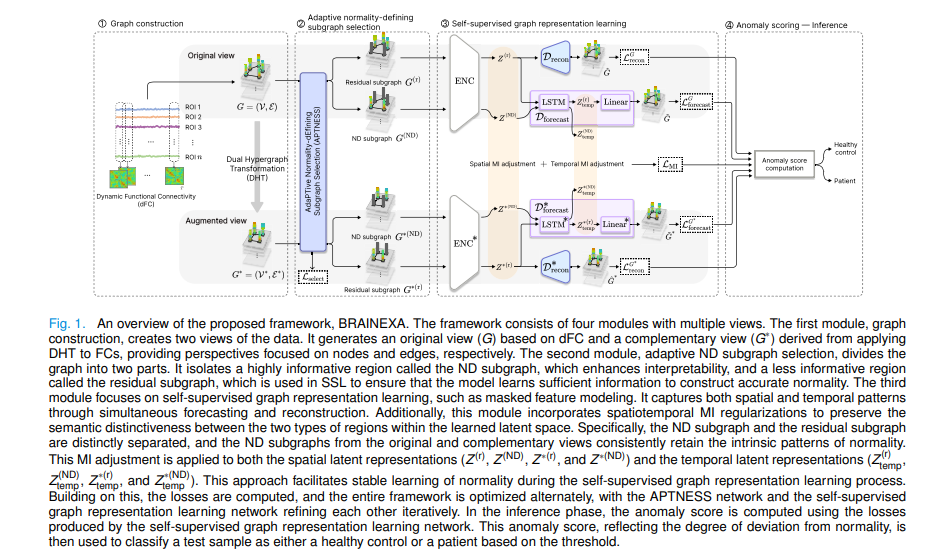
Korea University researchers built BRAINEXA, an unsupervised normative modeling framework that learns the spatiotemporal fingerprint of healthy brain connectivity from resting-state fMRI, then detects MDD, ASD, ADHD, and Alzheimer’s by measuring deviations — no diagnostic labels required during training, and clinically interpretable explanations included.
A psychiatrist reading a brain scan doesn’t start by looking for depression. They start by knowing what a healthy brain looks like — its resting connectivity patterns, its default-mode network rhythms, its temporal dynamics — and then they look for what’s wrong. This is normative reasoning: build a model of normal, then measure deviation. For decades, AI in neuroimaging has done the opposite, training classifiers on labeled datasets that require expensive expert annotation and that can only find what they were explicitly trained to look for. Yeajin Shon, Eunsong Kang, Da-Woon Heo, and Heung-Il Suk at Korea University built a system that reasons the way a clinician does — and explains its reasoning too.
The Label Problem in Brain Disorder AI
The dominant approach in computational psychiatry is supervised deep learning. Give the model a thousand fMRI scans labeled “MDD” and a thousand labeled “healthy,” train a classifier, deploy it. The results in the literature are often impressive, but the approach carries several structural weaknesses that limit real-world impact.
First, it can only detect what it’s been trained to detect. Subtle early-stage disruptions that don’t map cleanly onto diagnostic categories — the heterogeneous presentations, the prodromal states, the comorbidities — fall through the net. The model is optimizing for discriminative features tied to predefined labels, not for a comprehensive understanding of what healthy looks like.
Second, labeled clinical datasets are genuinely hard to obtain. Annotating psychiatric imaging data requires expert clinicians. The datasets are small by deep learning standards, often collected at single sites under specific protocols, and the labels themselves carry significant inter-rater variability.
Third — and this is the subtler problem — supervised learning discards a crucial resource: the enormous pool of healthy control data that exists across many research centers. Pooling healthy data across sites for normative modeling is relatively easy. Pooling patient data with consistent diagnostic labels is much harder.
Normative modeling inverts the problem. Train only on healthy controls — which are abundant, easily pooled across sites, and require no diagnostic labels. Then at inference, measure how much any new subject deviates from the learned norm. Large deviation means likely disorder. This approach can detect any deviation from normality, not just the specific disorders it was trained on, and it scales naturally as more healthy data becomes available.
Two Hard Problems in Normative Modeling for fMRI
The conceptual appeal of normative modeling is clear, but making it work on resting-state fMRI data faces two fundamental challenges that prior work hasn’t fully solved.
The first challenge is constructing normality accurately. Resting-state fMRI measures blood-oxygen-level-dependent (BOLD) signals across brain regions, and functional connectivity (FC) — typically estimated as Pearson correlation between region pairs — serves as the primary feature. But FC is inherently redundant: every correlation value between regions i and j appears in the feature vectors of both node i and node j in any graph representation. When self-supervised learning methods like masked autoencoders are applied to such redundant data, the model can trivially recover masked features by reading duplicated information from neighboring nodes. It learns shortcuts instead of normality.
The second challenge is explainability. Anomaly scores tell you how abnormal a subject is, but not why — which brain regions are deviating, whether those regions are functionally important, or whether the deviation constitutes a clinically meaningful disruption of normal brain function. In an unsupervised setting, building reliable explanations is substantially harder than in supervised classification where saliency maps and attention weights at least have a class prediction to explain.
BRAINEXA addresses both challenges through a carefully integrated four-module architecture.
The BRAINEXA Architecture: Four Modules Working Together
Module 1: Dynamic Functional Connectivity Graph Construction
Rather than treating the fMRI time series as a single static snapshot, BRAINEXA uses sliding windows to construct dynamic FC. The time series is partitioned into T overlapping segments (window size 50, step 45 in the experiments). For each segment t, Pearson correlations between all pairs of the 116 brain regions from the AAL atlas give the FC matrix \(X_t \in \mathbb{R}^{n \times n}\), which is sparsified by keeping the top 30% of connections. This yields a sequence of graphs \(\{G_t = (V_t, E_t)\}_{t=1}^T\).
To enable explanation at both node and edge levels, BRAINEXA also constructs an augmented graph \(G^*\) using Dual Hypergraph Transformation (DHT) — a bijective operation that transposes the incidence matrix, swapping the roles of nodes and edges. In the original graph, nodes are brain regions and edges are FC connections. In the augmented graph, nodes are FC connections and edges encode which regions they connect. This deterministic augmentation introduces no artificial noise and provides complementary structural perspectives for the explainability analysis.
Module 2: APTNESS — The Adaptive Subgraph Selector
This is the architectural innovation that solves the trivial learning problem. APTNESS (Adaptive Normality-Defining Subgraph Selector) divides the brain graph into two complementary parts: a normality-defining (ND) subgraph containing the most informative regions, and a residual subgraph containing the less informative remainder.
For each temporal segment, APTNESS encodes positional information using sinusoidal positional encoding, then passes the node features through multi-head self-attention followed by a Gumbel-Sigmoid function to produce a continuous probability score \(p \in \mathbb{R}^n\) for each node:
Hard thresholding at 0.5 converts these to binary decisions: nodes with \(p_i \geq 0.5\) become ND nodes (mask \(M^{(ND)}\)); the rest become residual nodes (mask \(M^{(r)}\)). For the augmented view, edge probabilities are derived from node probabilities via \(p^*_{e_{ij}} = p_i \cdot p_j\), ensuring structural consistency without a second selector network.
The training objective for APTNESS is to maximize the reconstruction and forecasting losses at the ND nodes — pushing the selector to identify the regions that are hardest to predict, i.e., the most informative ones:
While the reconstruction/forecasting network minimizes these losses, APTNESS maximizes them. This adversarial interplay forces the reconstruction network to actually learn the informative structure of normality rather than exploiting redundancy shortcuts.
Module 3: Spatiotemporal Self-Supervised Representation Learning
With the ND and residual subgraphs in hand, the core learning happens through two complementary SSL tasks applied to the residual subgraph — and evaluated at the ND indices.
Self-reconstruction uses a spatiotemporal graph convolutional (STGC) encoder to produce residual embeddings \(Z^{(r)}\), then reconstructs full node features via a decoder. Critically, the MSE loss is computed only at ND node indices (those identified as informative by APTNESS):
Forecasting addresses the limitation that reconstruction alone doesn’t capture temporal dynamics. Residual embeddings are fed into an LSTM to predict the next segment’s ND node features:
Spatiotemporal MI regularization is the third component. Encoding high-dimensional representations into lower-dimensional latent spaces can distort the semantic distinction between the ND and residual subgraphs. To prevent this, BRAINEXA applies InfoNCE (to maximize MI between ND subgraphs across views) and CLUB (to minimize MI between ND and residual subgraphs within each view):
Module 4: Anomaly Scoring and Explanation
At inference time, the reconstruction and forecasting losses for a test subject are compared against the Gaussian distribution of losses seen during training on healthy controls. A subject whose losses fall far in the tail of that distribution has brain dynamics that deviate significantly from the learned norm — a high anomaly score indicates likely disorder:
The ND subgraph from APTNESS provides the explanation: these are the brain regions that define normality. Regions with high anomaly scores and frequent ND membership are doubly flagged — they deviate from normal and they’re core to what normal means. This combination, unavailable in purely score-based anomaly detection, provides the clinically meaningful interpretation.
“While anomaly scores quantify the extent of deviation from normative patterns, ND subregions identify the specific components whose disruption most critically impairs normative brain function.” — Shon, Kang, Heo & Suk, IEEE TMI (2026)
Results: Better Than Supervised Methods, Without Seeing Any Labels
The experiments span four public datasets — REST-meta-MDD (MDD vs. healthy), ABIDE I (ASD vs. typically developing), ADHD-200 (ADHD vs. typically developing), and OASIS-3 (cognitive impairment vs. cognitively normal) — with site-balanced 10-fold cross-validation. BRAINEXA is compared against traditional statistical NM methods, supervised ML, supervised deep learning, and unsupervised deep learning baselines.
| Method | Category | REST-meta-MDD AUC | ABIDE I AUC | ADHD-200 AUC | OASIS-3 AUC |
|---|---|---|---|---|---|
| STIGR (best SDL) | Supervised DL | 0.713 | 0.720 | 0.672 | 0.812 |
| SIGNET | Unsup. DL | 0.663 | 0.680 | 0.672 | 0.811 |
| OmniAnomaly | Unsup. DL | 0.632 | 0.618 | 0.631 | 0.708 |
| GPR† | Normative | 0.464 | 0.459 | 0.456 | 0.480 |
| BRAINEXA | Normative (UDL) | 0.733 | 0.711 | 0.722 | 0.849 |
Table 1: Approximate AUC values from paper Table II. BRAINEXA outperforms the best supervised deep learning method (STIGR) by an average of 4.7% AUC across all four datasets, while requiring no diagnostic labels during training.
The result on the combined four-dataset experiment is particularly revealing. When all four datasets are pooled for training, supervised methods (SML and SDL) generally lose performance — the heterogeneous clinical categories confuse discriminative classifiers. Normative and unsupervised methods improve, because they benefit from seeing a wider distribution of healthy brain patterns. BRAINEXA shows the largest gains, confirming that its underlying approach — building a better model of normality — scales naturally with healthy data diversity.
The clinical validation is compelling: anomaly scores correlated with established clinical severity measures at \(|r| > 0.6\) across all four disorders (HAMD for MDD, ADOS for ASD, ADHD Index for ADHD, MMSE for Alzheimer’s). The model isn’t just detecting presence or absence of disorder — it’s reflecting symptom severity in its continuous anomaly scores.
What the Explanations Show
The ND subgraph analysis reveals neuroscientifically coherent patterns. In MDD, ND regions with high anomaly scores concentrate in the anterior cingulate cortex, amygdala, and temporal pole — structures involved in emotional regulation and affective processing, consistent with decades of depression neuroscience. In ASD, the supramarginal gyrus, superior temporal gyrus, and precuneus dominate — regions critical for social cognition and language processing. ADHD shows heightened anomalies in putamen, superior frontal gyrus, and cerebellar areas governing motor control and executive function. Alzheimer’s shows hippocampus, precuneus, and posterior cingulate — default mode network nodes whose disruption is a well-established biomarker of AD progression.
Across all datasets, hub regions including the thalamus, putamen, pallidum, and caudate appear consistently as ND nodes. These regions’ central role in neural transmission makes them natural anchors of normative brain organization. Their consistent selection by APTNESS — an unsupervised selector operating without any neuroanatomical prior — is a form of biological validation for the approach.
The ND subgraphs from the original and augmented views overlap at approximately 80% (Jaccard index) across all 10 folds and all datasets — a strong consistency result showing that APTNESS identifies stable, reproducible normality-defining structures rather than fitting noise.
Complete PyTorch Implementation of BRAINEXA
The implementation below covers every component of BRAINEXA: dynamic FC graph construction with DHT augmentation, the APTNESS adaptive subgraph selector with Gumbel-Sigmoid, the spatiotemporal graph convolutional encoder, self-reconstruction and LSTM-based forecasting decoders, spatiotemporal InfoNCE/CLUB mutual information regularization, the full alternating training loop (Algorithm 2), and anomaly scoring. A complete smoke test closes the file.
# ==============================================================================
# BRAINEXA: Explainable Normative Modeling for Brain Disorder Identification
# Paper: https://doi.org/10.1109/TMI.2025.3631105
# Authors: Shon, Kang, Heo, Suk (Korea University / Kangwon National University)
# Journal: IEEE Transactions on Medical Imaging, Vol. 45, No. 4, April 2026
# Code: https://github.com/ku-milab/BRAINEXA
# ==============================================================================
#
# Modules:
# 1. DualHypergraphTransform — DHT augmented graph construction
# 2. APTNESS — Adaptive ND subgraph selector (Eq. 1, 2, 13)
# 3. STGCLayer — Spatiotemporal graph convolution (Eq. 3)
# 4. STEncoder — Spatiotemporal VAE encoder
# 5. ReconDecoder — Reconstruction decoder (Eq. 4, 5)
# 6. ForecastDecoder — LSTM forecasting decoder (Eq. 6, 7)
# 7. MIRegularizer — InfoNCE + CLUB mutual information (Eq. 8–10)
# 8. BRAINEXA — Full model (Fig. 1)
# 9. BRAINEXATrainer — Alternating training loop (Algorithm 2)
# 10. AnomalyScorer — Gaussian anomaly scoring (Eq. 14)
# ==============================================================================
from __future__ import annotations
import warnings, math
import numpy as np
import torch
import torch.nn as nn
import torch.nn.functional as F
from torch.utils.data import Dataset, DataLoader
from typing import Dict, List, Optional, Tuple
from dataclasses import dataclass
warnings.filterwarnings('ignore')
torch.manual_seed(42)
# ─── SECTION 1: Configuration ─────────────────────────────────────────────────
@dataclass
class BRAINEXAConfig:
"""
Hyperparameters for BRAINEXA.
Parameters
----------
n_roi : number of ROIs (AAL atlas: 116)
window_size : sliding window size for dFC (paper: 50)
window_step : sliding window step (paper: 45)
top_k_pct : top-K% edges to keep for sparse FC (paper: 30%)
hidden_dim : STGC hidden dimension (paper: 32)
out_dim : STGC output / latent dimension (paper: 32)
gumbel_tau : Gumbel-Sigmoid temperature (paper: 0.5)
n_heads : MHSA heads in APTNESS
lstm_dim : LSTM output dimension for forecasting (paper: 32)
lr_main : learning rate for reconstruction/forecasting/MI network
lr_aptness : learning rate for APTNESS (same as lr_main in paper: 1e-4)
batch_size : mini-batch size (paper: 64)
n_epochs : total training epochs (paper: 100)
"""
n_roi: int = 116
window_size: int = 50
window_step: int = 45
top_k_pct: float = 0.3
hidden_dim: int = 32
out_dim: int = 32
gumbel_tau: float = 0.5
n_heads: int = 4
lstm_dim: int = 32
lr_main: float = 1e-4
lr_aptness: float = 1e-4
batch_size: int = 64
n_epochs: int = 100
device: str = 'cuda' if torch.cuda.is_available() else 'cpu'
# ─── SECTION 2: Graph Construction Utilities ──────────────────────────────────
def build_dynamic_fc(
bold: np.ndarray,
window_size: int = 50,
step: int = 45,
top_k_pct: float = 0.3,
) -> Tuple[List[np.ndarray], List[np.ndarray]]:
"""
Construct dynamic FC graphs from BOLD time series using sliding windows.
For each segment, computes Pearson correlation between ROI time series
and sparsifies by retaining the top K% of absolute correlation values.
Parameters
----------
bold : (n_roi, T_total) BOLD time series for one subject
window_size : frames per window
step : stride between window starts
top_k_pct : fraction of strongest connections to retain
Returns
-------
fc_matrices : list of (n_roi, n_roi) FC adjacency matrices per segment
node_feats : list of (n_roi, n_roi) node feature matrices (same as FC)
"""
n_roi, T = bold.shape
fc_list, feat_list = [], []
for start in range(0, T - window_size + 1, step):
segment = bold[:, start:start+window_size] # (n_roi, window_size)
fc = np.corrcoef(segment) # (n_roi, n_roi)
fc = np.nan_to_num(fc, nan=0.0)
np.fill_diagonal(fc, 0.0)
# Sparsify: keep top K% absolute values
threshold = np.percentile(np.abs(fc), (1 - top_k_pct) * 100)
adj = np.where(np.abs(fc) >= threshold, fc, 0.0)
fc_list.append(adj)
feat_list.append(adj.copy()) # node features = rows of FC matrix
return fc_list, feat_list
def dual_hypergraph_transform(
adj: torch.Tensor,
feat: torch.Tensor,
) -> Tuple[torch.Tensor, torch.Tensor]:
"""
Dual Hypergraph Transformation (DHT) — augmented view construction.
Swaps node/edge roles by transposing the incidence matrix.
Given original graph G with n nodes and m edges:
- Incidence matrix B ∈ {0,1}^{n×m}
- Dual graph G* has m nodes (original edges) and n edges (original nodes)
- Node features of G* are edge weights: X* ∈ R^{m×1}
This bijective, deterministic transformation provides a complementary
edge-centric view without introducing artificial noise, unlike perturbation
augmentations. It enables subsequent ND subgraph analysis at both node
and edge levels.
Parameters
----------
adj : (B_sz, n, n) adjacency matrices
feat : (B_sz, n, n) node feature matrices
Returns
-------
adj_star : (B_sz, m, m) dual adjacency (X* X*^T where X* = edge weights)
feat_star : (B_sz, m, 1) dual node features (edge weights as scalars)
"""
B_sz, n, _ = adj.shape
# Build incidence matrix from non-zero edges
incidence_list, feat_star_list, adj_star_list = [], [], []
for b in range(B_sz):
a = adj[b] # (n, n)
edge_idx = torch.nonzero(torch.triu(a, diagonal=1), as_tuple=False) # (m, 2)
if edge_idx.numel() == 0:
# Fallback: identity if no edges
adj_star_list.append(torch.eye(1, device=adj.device))
feat_star_list.append(torch.zeros(1, 1, device=adj.device))
continue
m = edge_idx.shape[0]
# Edge weights as dual node features
e_weights = a[edge_idx[:, 0], edge_idx[:, 1]].unsqueeze(1) # (m, 1)
# Dual adjacency: outer product of edge weights
adj_star = e_weights @ e_weights.t() # (m, m)
adj_star_list.append(adj_star)
feat_star_list.append(e_weights)
# Pad to uniform m across the batch (take max m)
max_m = max(f.shape[0] for f in feat_star_list)
padded_adj = torch.zeros(B_sz, max_m, max_m, device=adj.device)
padded_feat = torch.zeros(B_sz, max_m, 1, device=adj.device)
for b, (a_s, f_s) in enumerate(zip(adj_star_list, feat_star_list)):
m_b = f_s.shape[0]
padded_adj[b, :m_b, :m_b] = a_s
padded_feat[b, :m_b, :] = f_s
return padded_adj, padded_feat
# ─── SECTION 3: APTNESS — Adaptive ND Subgraph Selector ───────────────────────
class GumbelSigmoid(nn.Module):
"""
Gumbel-Sigmoid activation for differentiable discrete selection (Algorithm 1).
During training: adds Gumbel noise and passes through sigmoid for
continuous relaxation that enables gradient-based optimization.
During inference: uses hard thresholding at 0.5 without noise.
Temperature τ controls the sharpness of the approximation:
lower τ → closer to hard binary decisions.
"""
def __init__(self, tau: float = 0.5) -> None:
super().__init__()
self.tau = tau
def forward(self, logits: torch.Tensor) -> torch.Tensor:
if self.training:
g = -torch.log(-torch.log(torch.rand_like(logits).clamp(1e-10)))
return torch.sigmoid((logits + g) / self.tau)
else:
return torch.sigmoid(logits / self.tau)
class APTNESS(nn.Module):
"""
Adaptive Normality-Defining Subgraph Selector (Section III-B, Algorithm 1).
Assigns probability scores to each node, then hard-thresholds to
binary ND (1) or residual (0) membership.
Architecture:
Sinusoidal positional encoding + MHSA + Linear → Gumbel-Sigmoid → p ∈ R^n
The APTNESS is optimized to MAXIMIZE reconstruction/forecasting losses
at ND nodes (Eq. 13), pushing the selector to identify informative regions.
This adversarial objective makes ND nodes the hardest to predict from
residual nodes, preventing trivial SSL solutions due to FC redundancy.
Parameters
----------
n_feat : node feature dimension (n_roi for original view)
n_heads : number of MHSA heads
tau : Gumbel-Sigmoid temperature
"""
def __init__(self, n_feat: int, n_heads: int = 4, tau: float = 0.5) -> None:
super().__init__()
self.n_feat = n_feat
# Sinusoidal positional encoding (fixed)
pe = self._build_pe(n_feat, n_feat)
self.register_buffer('pos_enc', pe)
# Multi-head self-attention over nodes
self.mhsa = nn.MultiheadAttention(n_feat, n_heads, batch_first=True)
self.linear = nn.Linear(n_feat, 1)
self.gumbel = GumbelSigmoid(tau)
@staticmethod
def _build_pe(n_pos: int, d_model: int) -> torch.Tensor:
"""Sinusoidal positional encoding (n_pos, d_model)."""
pe = torch.zeros(n_pos, d_model)
pos = torch.arange(0, n_pos, dtype=torch.float).unsqueeze(1)
div = torch.exp(torch.arange(0, d_model, 2, dtype=torch.float) * (-math.log(10000.0) / d_model))
pe[:, 0::2] = torch.sin(pos * div)
pe[:, 1::2] = torch.cos(pos * div[:d_model//2])
return pe
def forward(self, X: torch.Tensor) -> Tuple[torch.Tensor, torch.Tensor, torch.Tensor]:
"""
Compute node probability scores and subgraph masks.
Parameters
----------
X : (B, n_roi, n_feat) node feature matrix
Returns
-------
p : (B, n_roi) continuous probability scores in (0,1)
mask_nd : (B, n_roi) binary ND mask (1=ND node, 0=residual)
mask_r : (B, n_roi) binary residual mask
"""
B, n, _ = X.shape
# Add positional encoding
X0 = X + self.pos_enc[:n, :X.shape[-1]].unsqueeze(0)
# MHSA → linear → Gumbel-Sigmoid
attn_out, _ = self.mhsa(X0, X0, X0)
logits = self.linear(attn_out).squeeze(-1) # (B, n)
p = self.gumbel(logits) # (B, n) ∈ (0,1)
# Hard thresholding for discrete masks
mask_nd = (p >= 0.5).float()
mask_r = 1.0 - mask_nd
return p, mask_nd, mask_r
def edge_probabilities(self, p: torch.Tensor) -> Tuple[torch.Tensor, torch.Tensor]:
"""
Map node probabilities to edge probabilities for augmented view (Eq. 2).
p*_{e_ij} = p_i * p_j
Parameters
----------
p : (B, n_roi) node probability scores
Returns
-------
p_star : (B, m) edge probability scores (outer product flattened)
mask_nd* : (B, m) binary ND edge mask
"""
# Outer product for all node pairs → edge scores
p_mat = p.unsqueeze(2) * p.unsqueeze(1) # (B, n, n)
# Flatten upper triangle for edge-level scores
B, n, _ = p_mat.shape
mask = torch.triu(torch.ones(n, n, device=p.device), diagonal=1).bool()
p_star = p_mat[:, mask] # (B, m)
mask_nd_star = (p_star >= 0.5).float()
return p_star, mask_nd_star
# ─── SECTION 4: Spatiotemporal Graph Convolution ──────────────────────────────
class STGCLayer(nn.Module):
"""
Spatiotemporal Graph Convolution layer (Eq. 3).
Combines:
Spatial: normalized graph convolution Λ^{-½}(A+I)Λ^{-½} H W_spa
Temporal: 1D convolution along the T-axis W_temp
H^{(l+1)}_spa = ReLU(Λ^{-½}(A+I)Λ^{-½} H^{(l)} W_spa)
H^{(l+1)} = ReLU(Dropout(BN(H^{(l+1)}_spa * W_temp)))
Parameters
----------
in_ch : input feature channels
out_ch : output feature channels
temp_kernel: 1D conv kernel size along temporal axis
"""
def __init__(self, in_ch: int, out_ch: int, temp_kernel: int = 3, dropout: float = 0.1) -> None:
super().__init__()
self.W_spa = nn.Linear(in_ch, out_ch, bias=False)
self.W_temp = nn.Conv1d(out_ch, out_ch, kernel_size=temp_kernel, padding=temp_kernel//2, bias=False)
self.bn = nn.BatchNorm1d(out_ch)
self.dropout = nn.Dropout(dropout)
def _normalize_adj(self, A: torch.Tensor) -> torch.Tensor:
"""Compute Λ^{-½}(A+I)Λ^{-½} for batched adjacency matrices."""
B, n, _ = A.shape
I = torch.eye(n, device=A.device).unsqueeze(0).expand(B, -1, -1)
A_hat = A + I
deg = A_hat.sum(dim=-1).clamp(min=1e-6)
D_inv_sqrt = torch.diag_embed(deg.pow(-0.5))
return D_inv_sqrt @ A_hat @ D_inv_sqrt
def forward(self, H: torch.Tensor, A: torch.Tensor) -> torch.Tensor:
"""
Parameters
----------
H : (B, n, d_in) node features stacked over T segments, or (B, n, T, d_in)
A : (B, n, n) adjacency matrix
Returns
-------
H_out : (B, n, d_out)
"""
A_norm = self._normalize_adj(A)
# Spatial convolution
H_spa = F.relu(self.W_spa(A_norm @ H)) # (B, n, out_ch)
# Temporal convolution along node dimension (treat n as sequence)
H_t = H_spa.transpose(1, 2) # (B, out_ch, n)
H_t = self.W_temp(H_t).transpose(1, 2) # (B, n, out_ch)
H_t = self.bn(H_t.reshape(-1, H_t.shape[-1])).reshape(H_t.shape)
H_out = F.relu(self.dropout(H_t))
return H_out
# ─── SECTION 5: Encoder, Decoders ─────────────────────────────────────────────
class STEncoder(nn.Module):
"""
Spatiotemporal encoder: two STGC layers → latent Z ∈ R^{n×d}.
Takes (residual or ND) subgraph features and adjacency, returns
lower-dimensional latent representation used for all SSL tasks.
"""
def __init__(self, in_ch: int, hidden: int, out_ch: int) -> None:
super().__init__()
self.stgc1 = STGCLayer(in_ch, hidden)
self.stgc2 = STGCLayer(hidden, out_ch)
def forward(self, X: torch.Tensor, A: torch.Tensor) -> torch.Tensor:
return self.stgc2(self.stgc1(X, A), A)
class ReconDecoder(nn.Module):
"""
Reconstruction decoder: STGC layer + fully connected → reconstructed X̂ (Eq. 4).
Takes residual subgraph embedding Z^{(r)} and reconstructs the full
node feature matrix. Loss is evaluated only at ND node indices (Eq. 5).
"""
def __init__(self, in_ch: int, out_ch: int) -> None:
super().__init__()
self.stgc = STGCLayer(in_ch, in_ch, temp_kernel=1)
self.fc = nn.Sequential(nn.Linear(in_ch, out_ch), nn.Tanh())
def forward(self, Z: torch.Tensor, A: torch.Tensor) -> torch.Tensor:
h = self.stgc(Z, A)
return self.fc(h)
class ForecastDecoder(nn.Module):
"""
Forecasting decoder: LSTM over temporal embeddings + Linear → X̃_{t+1} (Eq. 6).
Captures temporal evolution patterns in dFC that self-reconstruction alone
cannot model. Takes residual embeddings across T segments as a sequence.
Loss evaluated at ND node indices for next segment (Eq. 7).
"""
def __init__(self, in_ch: int, lstm_dim: int, out_ch: int) -> None:
super().__init__()
self.lstm = nn.LSTM(in_ch, lstm_dim, batch_first=True)
self.linear = nn.Linear(lstm_dim, out_ch)
def forward(self, Z_seq: torch.Tensor) -> Tuple[torch.Tensor, torch.Tensor]:
"""
Parameters
----------
Z_seq : (B, T, n_feat) sequence of residual embeddings (mean-pooled over nodes)
Returns
-------
X_forecast : (B, T, out_ch) predicted node features for next segment
Z_temp : (B, T, lstm_dim) temporal latent representations
"""
Z_temp, _ = self.lstm(Z_seq) # (B, T, lstm_dim)
X_forecast = self.linear(Z_temp) # (B, T, out_ch)
return X_forecast, Z_temp
# ─── SECTION 6: Mutual Information Regularization ─────────────────────────────
class InfoNCELoss(nn.Module):
"""
InfoNCE contrastive loss for MI maximization (Eq. 8 — LInfo term).
Maximizes mutual information between corresponding representations
(e.g., ND subgraph from original and augmented views) by pulling
matched pairs together and pushing unmatched pairs apart.
I(Z^{(ND)}; Z^{*(ND)}) → minimize L_InfoNCE = -E[log(sim(+) / Σ sim(-))]
"""
def __init__(self, temperature: float = 0.1) -> None:
super().__init__()
self.tau = temperature
def forward(self, z1: torch.Tensor, z2: torch.Tensor) -> torch.Tensor:
"""
Parameters
----------
z1, z2 : (B, d) paired representations to align
Returns
-------
loss : InfoNCE scalar (lower → higher MI)
"""
z1 = F.normalize(z1, dim=-1)
z2 = F.normalize(z2, dim=-1)
sim = z1 @ z2.t() / self.tau # (B, B)
labels = torch.arange(z1.size(0), device=z1.device)
loss = (0.5 * F.cross_entropy(sim, labels) +
0.5 * F.cross_entropy(sim.t(), labels))
return loss
class CLUBLoss(nn.Module):
"""
CLUB (Contrastive Log-ratio Upper Bound) for MI minimization (Eq. 8 — LCLUB term).
Minimizes mutual information between ND and residual subgraph representations
within each view, enforcing semantic distinctiveness between the two regions.
I(Z^{(r)}; Z^{(ND)}) → maximize L_CLUB = E[log p(z_nd|z_r)] - E[log p(z_nd'|z_r)]
"""
def __init__(self, d: int) -> None:
super().__init__()
# Variational network to estimate conditional p(z_nd | z_r)
self.mu_net = nn.Sequential(nn.Linear(d, d), nn.ReLU(), nn.Linear(d, d))
self.logvar_net = nn.Sequential(nn.Linear(d, d), nn.ReLU(), nn.Linear(d, d))
def forward(self, z_r: torch.Tensor, z_nd: torch.Tensor) -> torch.Tensor:
"""
Parameters
----------
z_r : (B, d) residual subgraph embeddings (conditioning variable)
z_nd : (B, d) ND subgraph embeddings (to minimize dependence on)
Returns
-------
loss : CLUB upper bound (minimize to reduce MI)
"""
mu = self.mu_net(z_r)
logvar = self.logvar_net(z_r).clamp(-10, 10)
# log p(z_nd | z_r) for each positive pair
pos_logprob = -0.5 * (((z_nd - mu) ** 2) / logvar.exp() + logvar).sum(dim=-1)
# log p(z_nd' | z_r) for random negative pairs (shuffle)
B = z_nd.shape[0]
idx = torch.randperm(B, device=z_nd.device)
neg_logprob = -0.5 * (((z_nd[idx] - mu) ** 2) / logvar.exp() + logvar).sum(dim=-1)
return (pos_logprob - neg_logprob).mean()
class MIRegularizer(nn.Module):
"""
Spatiotemporal Mutual Information regularization (Eqs. 8–10).
Within each view: MINIMIZE MI between ND and residual subgraphs
→ ensures semantic distinctiveness (CLUB)
Across views: MAXIMIZE MI between ND subgraphs
→ ensures consistent normality encoding (InfoNCE)
Applied to both spatial (STGC) and temporal (LSTM) latent representations.
L_spa = L_Info(Z^{(ND)};Z^{*(ND)}) + L_CLUB(Z^{(r)};Z^{(ND)}) + L_CLUB(Z^{*(r)};Z^{*(ND)})
L_temp = L_Info(Z^{(ND)}_temp;Z^{*(ND)}_temp) + ... (analogous)
L_MI = L_spa + L_temp
"""
def __init__(self, d: int) -> None:
super().__init__()
self.infonce = InfoNCELoss()
self.club_orig = CLUBLoss(d)
self.club_aug = CLUBLoss(d)
def forward(
self,
Z_nd: torch.Tensor, Z_r: torch.Tensor,
Z_nd_star: torch.Tensor, Z_r_star: torch.Tensor,
) -> torch.Tensor:
"""
Compute MI regularization loss for one modality (spatial or temporal).
Parameters
----------
Z_nd : (B, d) ND embeddings from original view
Z_r : (B, d) residual embeddings from original view
Z_nd_star : (B, d) ND embeddings from augmented view
Z_r_star : (B, d) residual embeddings from augmented view
Returns
-------
L_MI_component : scalar MI regularization loss
"""
L_info = self.infonce(Z_nd, Z_nd_star) # maximize cross-view MI
L_club1 = self.club_orig(Z_r, Z_nd) # minimize within-view MI (orig)
L_club2 = self.club_aug(Z_r_star, Z_nd_star) # minimize within-view MI (aug)
return L_info + L_club1 + L_club2
# ─── SECTION 7: Full BRAINEXA Model ───────────────────────────────────────────
class BRAINEXA(nn.Module):
"""
BRAINEXA: Normative Explanatory Analysis for BRAIN disorders (Fig. 1).
Four-module architecture:
1. Graph construction (preprocessing — handled externally)
2. APTNESS: adaptive ND/residual subgraph selection (Eq. 1, 2)
3. Self-supervised graph representation learning:
- STEncoder → Z^{(r)}, Z^{(ND)}, Z^{*(r)}, Z^{*(ND)}
- ReconDecoder: X̂ from Z^{(r)}, loss at ND indices (Eq. 5)
- ForecastDecoder: X̃_{t+1} from Z^{(r)}_temp, loss at ND indices (Eq. 7)
- MIRegularizer: spatiotemporal InfoNCE + CLUB (Eq. 8–10)
4. Anomaly scoring (Eq. 14, in AnomalyScorer)
The model is trained exclusively on healthy control data.
At inference, anomaly score reflects deviation from learned normality.
ND subgraphs from APTNESS provide region-level explanations.
Parameters
----------
cfg : BRAINEXAConfig
"""
def __init__(self, cfg: BRAINEXAConfig) -> None:
super().__init__()
self.cfg = cfg
n = cfg.n_roi
h = cfg.hidden_dim
d = cfg.out_dim
# Module 2: APTNESS
self.aptness = APTNESS(n, cfg.n_heads, cfg.gumbel_tau)
# Module 3a: Encoders for original and augmented views
self.enc = STEncoder(n, h, d) # original view
self.enc_s = STEncoder(1, h, d) # augmented view (1D edge features)
# Module 3b: Reconstruction decoders
self.recon = ReconDecoder(d, n)
self.recon_s = ReconDecoder(d, 1)
# Module 3c: Forecasting decoders
self.forecast = ForecastDecoder(d, cfg.lstm_dim, n)
self.forecast_s = ForecastDecoder(d, cfg.lstm_dim, 1)
# Module 3d: MI regularizers (spatial and temporal)
self.mi_spa = MIRegularizer(d)
self.mi_temp = MIRegularizer(cfg.lstm_dim)
def forward(
self,
X: torch.Tensor, # (B, n, n) node features (dFC row = node feat)
A: torch.Tensor, # (B, n, n) adjacency matrix
A_star: torch.Tensor, # (B, m, m) dual hypergraph adjacency
X_star: torch.Tensor, # (B, m, 1) dual hypergraph node features
) -> Dict:
"""
Single-segment forward pass. For T-segment dFC, call for each t.
Returns
-------
Dictionary with:
'Z_nd', 'Z_r' : spatial latents for original view
'Z_nd_star','Z_r_star' : spatial latents for augmented view
'X_hat' : reconstructed features (original)
'X_hat_star' : reconstructed features (augmented)
'mask_nd', 'mask_r' : ND/residual masks (original)
'p' : node probability scores
"""
# ── APTNESS: subgraph selection ──
p, mask_nd, mask_r = self.aptness(X) # (B,n) each
# Apply masks to node features
X_nd = X * mask_nd.unsqueeze(-1) # (B, n, n) ND features
X_r = X * mask_r.unsqueeze(-1) # (B, n, n) residual features
# ── Encode subgraphs ──
Z_nd = self.enc(X_nd, A) # (B, n, d)
Z_r = self.enc(X_r, A) # (B, n, d)
# ── Augmented view APTNESS via probability mapping (Eq. 2) ──
_, mask_nd_star = self.aptness.edge_probabilities(p) # (B, m)
# Augmented view has 1D features; expand mask accordingly
m = X_star.shape[1]
mask_nd_s_full = mask_nd_star[:, :m].unsqueeze(-1)
mask_r_s_full = 1.0 - mask_nd_s_full
X_nd_star = X_star * mask_nd_s_full
X_r_star = X_star * mask_r_s_full
Z_nd_star = self.enc_s(X_nd_star, A_star) # (B, m, d)
Z_r_star = self.enc_s(X_r_star, A_star) # (B, m, d)
# ── Reconstruct from residual embeddings (Eq. 4) ──
X_hat = self.recon(Z_r, A) # (B, n, n)
X_hat_star = self.recon_s(Z_r_star, A_star) # (B, m, 1)
return {
'Z_nd': Z_nd, 'Z_r': Z_r,
'Z_nd_star': Z_nd_star, 'Z_r_star': Z_r_star,
'X_hat': X_hat, 'X_hat_star': X_hat_star,
'mask_nd': mask_nd, 'mask_r': mask_r,
'mask_nd_star': mask_nd_star[:, :m],
'p': p,
}
def compute_losses(
self,
outputs: Dict,
X_target: torch.Tensor, # (B, n, n) ground truth
X_target_star: torch.Tensor, # (B, m, 1) ground truth (augmented)
X_next: Optional[torch.Tensor] = None, # next segment for forecasting
X_next_star: Optional[torch.Tensor] = None,
) -> Dict[str, torch.Tensor]:
"""
Compute all loss components for one segment.
Parameters
----------
outputs : dict from forward()
X_target : ground-truth node features for current segment
X_target_star : ground-truth dual node features
X_next : ground-truth node features for next segment (for forecasting)
X_next_star : ground-truth dual node features for next segment
Returns
-------
losses : dict with 'recon', 'forecast', 'mi', 'select', 'total'
"""
mask_nd = outputs['mask_nd'].unsqueeze(-1)
# Reconstruction loss (Eq. 5): MSE at ND indices only
L_recon = (mask_nd * (outputs['X_hat'] - X_target) ** 2).mean()
mask_nd_s = outputs['mask_nd_star'].unsqueeze(-1)
L_recon_s = (mask_nd_s * (outputs['X_hat_star'] - X_target_star) ** 2).mean()
L_total_recon = L_recon + L_recon_s
# Forecasting loss (Eq. 7): if next segment provided
L_forecast = torch.tensor(0.0, device=X_target.device)
if X_next is not None:
# Single-step forecast using temporal mean of Z_r as sequence proxy
Z_r_seq = outputs['Z_r'].mean(dim=1, keepdim=True) # (B,1,d)
X_pred_next, _ = self.forecast(Z_r_seq)
X_pred_next = X_pred_next.squeeze(1) # (B, n)
X_next_target = (X_next * mask_nd.squeeze(-1)).mean(dim=-1)
L_forecast = F.mse_loss(
X_pred_next * mask_nd.squeeze(-1)[:, :, 0],
X_next_target
)
# MI regularization (Eq. 8–10)
Z_nd_pool = outputs['Z_nd'].mean(dim=1) # (B, d)
Z_r_pool = outputs['Z_r'].mean(dim=1)
Z_nd_s_pool= outputs['Z_nd_star'].mean(dim=1)
Z_r_s_pool = outputs['Z_r_star'].mean(dim=1)
L_mi = self.mi_spa(Z_nd_pool, Z_r_pool, Z_nd_s_pool, Z_r_s_pool)
# APTNESS selection loss (Eq. 13): maximize at ND nodes
p_nd = outputs['p'] * outputs['mask_nd'] # (B, n)
L_select = (p_nd.mean(dim=-1) * L_recon.detach()).mean()
L_total = L_total_recon + L_forecast + L_mi
return {
'recon': L_total_recon, 'forecast': L_forecast,
'mi': L_mi, 'select': L_select, 'total': L_total,
}
# ─── SECTION 8: Training Loop (Algorithm 2) ───────────────────────────────────
class BRAINEXATrainer:
"""
Alternating training loop for BRAINEXA (Algorithm 2).
Two parameter groups are updated alternately:
φ (reconstruction, forecasting, MI network): minimize total loss
θ (APTNESS): maximize selection loss (gradient ASCENT)
This adversarial interplay ensures APTNESS continuously identifies harder
prediction targets, preventing the SSL network from exploiting shortcuts.
Parameters
----------
model : BRAINEXA instance
cfg : BRAINEXAConfig
"""
def __init__(self, model: BRAINEXA, cfg: BRAINEXAConfig) -> None:
self.model = model.to(cfg.device)
self.cfg = cfg
self.device = cfg.device
# φ: all parameters EXCEPT APTNESS
aptness_ids = set(id(p) for p in model.aptness.parameters())
phi_params = [p for p in model.parameters() if id(p) not in aptness_ids]
theta_params = list(model.aptness.parameters())
self.opt_phi = torch.optim.Adam(phi_params, lr=cfg.lr_main)
self.opt_theta = torch.optim.Adam(theta_params, lr=cfg.lr_aptness)
def train_step(
self,
X_batch: torch.Tensor,
A_batch: torch.Tensor,
A_star_batch: torch.Tensor,
X_star_batch: torch.Tensor,
X_next_batch: Optional[torch.Tensor] = None,
X_next_star: Optional[torch.Tensor] = None,
) -> Dict[str, float]:
"""
One training iteration: update φ (minimize), then θ (maximize).
Parameters
----------
X_batch : (B, n, n) node features for current segments
A_batch : (B, n, n) adjacency matrices
A_star_batch : (B, m, m) dual adjacency matrices
X_star_batch : (B, m, 1) dual node features
X_next_batch : (B, n, n) ground truth for next segment (optional)
X_next_star : (B, m, 1) dual gt for next segment (optional)
Returns
-------
loss_dict : dict with scalar loss values for logging
"""
X = X_batch.to(self.device)
A = A_batch.to(self.device)
A_s = A_star_batch.to(self.device)
X_s = X_star_batch.to(self.device)
X_nxt = X_next_batch.to(self.device) if X_next_batch is not None else None
X_ns = X_next_star.to(self.device) if X_next_star is not None else None
# ── Step 1: Update φ — minimize total loss ──
self.opt_phi.zero_grad()
outputs = self.model(X, A, A_s, X_s)
losses = self.model.compute_losses(outputs, X, X_s, X_nxt, X_ns)
losses['total'].backward()
self.opt_phi.step()
# ── Step 2: Update θ — maximize selection loss ──
self.opt_theta.zero_grad()
outputs2 = self.model(X, A, A_s, X_s)
losses2 = self.model.compute_losses(outputs2, X, X_s, X_nxt, X_ns)
(-losses2['select']).backward() # gradient ASCENT on L_select
self.opt_theta.step()
return {k: v.item() for k, v in losses.items()}
def fit(
self,
dataloader: DataLoader,
verbose: bool = True,
) -> List[Dict]:
"""
Full training for n_epochs epochs on healthy control data only.
Parameters
----------
dataloader : yields (X, A, A_star, X_star) or (X, A, A_star, X_star, X_next, X_next_star)
verbose : print per-epoch progress
Returns
-------
history : list of per-epoch loss dicts
"""
history = []
if verbose:
print(f"\n── BRAINEXA Training ─────────────────────────────────────")
print(f" Device: {self.cfg.device} | Epochs: {self.cfg.n_epochs}")
for epoch in range(1, self.cfg.n_epochs + 1):
self.model.train()
epoch_losses: Dict[str, float] = {}
for batch in dataloader:
if len(batch) == 4:
step_losses = self.train_step(*batch)
else:
step_losses = self.train_step(*batch[:4], batch[4], batch[5])
for k, v in step_losses.items():
epoch_losses[k] = epoch_losses.get(k, 0) + v
epoch_losses = {k: v / len(dataloader) for k, v in epoch_losses.items()}
history.append({'epoch': epoch, **epoch_losses})
if verbose and epoch % 10 == 0:
print(f" Epoch {epoch:4} | recon={epoch_losses['recon']:.4f} | mi={epoch_losses['mi']:.4f} | total={epoch_losses['total']:.4f}")
if verbose:
print("✓ Training complete.")
return history
# ─── SECTION 9: Anomaly Scoring ───────────────────────────────────────────────
class AnomalyScorer:
"""
Gaussian anomaly scoring for test subjects (Eq. 14).
During training: records the empirical mean and std of all loss components.
During inference: computes the Gaussian log-likelihood of observed losses
under the training distribution. Low likelihood → high anomaly score.
S = exp(-N(L^G_recon) - N(L^{G*}_recon) - N(L^G_forecast) - N(L^{G*}_forecast)
- N(L_spa) - N(L_temp))
where N(·) denotes the Gaussian CDF/log-density of training losses.
Classification threshold is determined using Youden's index on a
validation set (healthy controls and patients with known labels).
"""
def __init__(self) -> None:
self.train_stats: Optional[Dict[str, Tuple[float, float]]] = None
def fit(self, train_losses: List[Dict[str, float]]) -> None:
"""
Record mean and std of training losses for Gaussian modeling.
Parameters
----------
train_losses : list of loss dicts from training (one per sample/segment)
"""
keys = train_losses[0].keys()
self.train_stats = {}
for k in keys:
vals = np.array([l[k] for l in train_losses])
self.train_stats[k] = (np.mean(vals), np.std(vals) + 1e-8)
def score(self, test_losses: Dict[str, float]) -> float:
"""
Compute anomaly score for a single test subject (Eq. 14).
Parameters
----------
test_losses : dict of loss values at inference time
Returns
-------
anomaly_score : float in (0, 1], higher = more abnormal
"""
if self.train_stats is None:
raise RuntimeError("Call fit() before score().")
log_prob = 0.0
for k, val in test_losses.items():
if k in self.train_stats:
mu, sigma = self.train_stats[k]
log_prob += -0.5 * ((val - mu) / sigma) ** 2
return float(np.exp(log_prob))
# ─── SECTION 10: Smoke Test ───────────────────────────────────────────────────
if __name__ == '__main__':
print("=" * 62)
print("BRAINEXA — Smoke Test (Synthetic Data)")
print("=" * 62)
np.random.seed(42)
# Small config for quick test
cfg = BRAINEXAConfig(
n_roi=20, window_size=20, window_step=10,
hidden_dim=16, out_dim=16, lstm_dim=16,
n_heads=2, batch_size=4, n_epochs=3,
)
n, d = cfg.n_roi, cfg.out_dim
# ── Test 1: Dynamic FC construction ──
print(f"\n[1/5] Dynamic FC construction...")
bold = np.random.randn(n, 100) # (n_roi, T_total)
fc_list, feat_list = build_dynamic_fc(bold, cfg.window_size, cfg.window_step, cfg.top_k_pct)
print(f" {len(fc_list)} segments, each ({n}, {n})")
# ── Test 2: DHT augmented view ──
print(f"\n[2/5] Dual Hypergraph Transform...")
A_b = torch.tensor(fc_list[0], dtype=torch.float32).unsqueeze(0).expand(cfg.batch_size, -1, -1)
X_b = torch.tensor(feat_list[0], dtype=torch.float32).unsqueeze(0).expand(cfg.batch_size, -1, -1)
A_star, X_star = dual_hypergraph_transform(A_b, X_b)
print(f" Original: nodes={n}, edges~{int(A_star.shape[1])}")
print(f" Dual: X_star={tuple(X_star.shape)}, A_star={tuple(A_star.shape)}")
# ── Test 3: APTNESS subgraph selection ──
print(f"\n[3/5] APTNESS subgraph selection...")
aptness = APTNESS(n, cfg.n_heads, cfg.gumbel_tau)
p, mask_nd, mask_r = aptness(X_b)
n_nd = mask_nd.sum(dim=-1).mean().item()
print(f" Prob scores: min={p.min():.3f}, max={p.max():.3f}")
print(f" Avg ND nodes per sample: {n_nd:.1f} / {n}")
assert mask_nd.shape == (cfg.batch_size, n), "APTNESS mask shape error"
# ── Test 4: Full model forward pass ──
print(f"\n[4/5] BRAINEXA forward pass + loss computation...")
model = BRAINEXA(cfg)
n_params = sum(p.numel() for p in model.parameters())
print(f" Parameters: {n_params:,}")
outputs = model(X_b, A_b, A_star, X_star)
losses = model.compute_losses(outputs, X_b, X_star)
print(f" Losses: recon={losses['recon'].item():.4f} | mi={losses['mi'].item():.4f} | select={losses['select'].item():.4f}")
assert outputs['Z_nd'].shape == (cfg.batch_size, n, d), "Z_nd shape error"
print(" ✓ Forward pass and losses OK")
# ── Test 5: Mini training loop ──
print(f"\n[5/5] Mini alternating training loop ({cfg.n_epochs} epochs)...")
# Synthetic dataset of 8 healthy control samples
class SyntheticFCDataset(Dataset):
def __init__(self, n_samples, n_roi, batch_size):
self.n = n_samples
self.n_roi = n_roi
def __len__(self): return self.n
def __getitem__(self, i):
X = torch.randn(self.n_roi, self.n_roi)
A = torch.abs(X)
A_s, X_s = dual_hypergraph_transform(A.unsqueeze(0), X.unsqueeze(0))
return X, A, A_s.squeeze(0), X_s.squeeze(0)
dataset = SyntheticFCDataset(16, n, cfg.batch_size)
loader = DataLoader(dataset, batch_size=cfg.batch_size, shuffle=True)
trainer = BRAINEXATrainer(model, cfg)
history = trainer.fit(loader, verbose=True)
print(f" Final epoch loss: {history[-1]['total']:.4f}")
# ── Anomaly scoring ──
scorer = AnomalyScorer()
train_loss_records = [{'recon': np.random.uniform(0.1, 0.3), 'mi': np.random.uniform(0.05, 0.15), 'select': np.random.uniform(0.01, 0.05)} for _ in range(50)]
scorer.fit(train_loss_records)
normal_score = scorer.score({'recon': 0.18, 'mi': 0.09, 'select': 0.02})
anomaly_score = scorer.score({'recon': 0.95, 'mi': 0.60, 'select': 0.40})
print(f"\n── Anomaly Scoring ──────────────────────────────────────────")
print(f" Healthy control score: {normal_score:.4f} (should be higher)")
print(f" Disorder patient score: {anomaly_score:.6f} (should be lower → more abnormal)")
print(f"\n✓ All BRAINEXA checks passed.")
print("=" * 62)
Read the Full Paper & Access the Code
BRAINEXA is published open-access in IEEE Transactions on Medical Imaging under CC BY 4.0. The official PyTorch implementation with pretrained models and dataset preprocessing scripts is available on GitHub.
Shon, Y., Kang, E., Heo, D.-W., & Suk, H.-I. (2026). Explainable normative modeling for brain disorder identification in resting-state fMRI. IEEE Transactions on Medical Imaging, 45(4), 1606–1619. https://doi.org/10.1109/TMI.2025.3631105
This article is an independent editorial analysis of peer-reviewed research. The PyTorch implementation is an educational reproduction of the paper’s methodology. The official implementation is at github.com/ku-milab/BRAINEXA. Supported by IITP/MSIT Korea under Grant RS-2024-00457882.
Explore More on AI Trend Blend
From medical AI and neuroimaging to manufacturing intelligence, federated learning security, and precision agriculture — here is the full scope of what we cover.