Key points
- CHAKG projects both a knowledge graph and a user item interaction graph into a shared space made of learned hyperedges, letting it spot groups of semantically related items without expensive multi hop graph traversal.
- Once it finds a long tail item with a strongly related, meaningfully more popular partner item, it borrows a portion of that partner’s real user interactions and assigns them to the long tail item as extra training signal.
- A learned consistency gate checks each borrowed interaction against both the collaborative and knowledge graph signals before trusting it, filtering out transfers that would inject noise.
- A cross modal contrastive loss keeps the knowledge graph view and the interaction view of every item pointing in a semantically consistent direction.
- Across four benchmark datasets, CHAKG beats the strongest prior baseline by an average of 5.3 percent on Recall@20 and 4.8 percent on NDCG@20, with the largest gains concentrated specifically on long tail items rather than already popular ones.
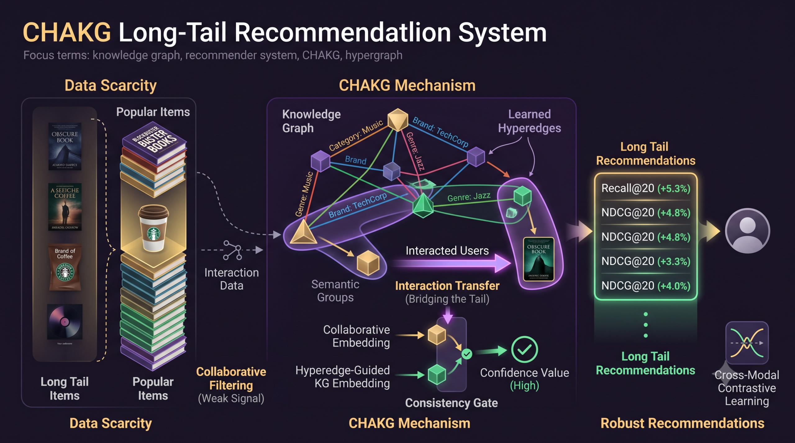
The core problem, why a knowledge graph alone does not fix the long tail
Most real recommendation catalogs are lopsided by design. A small number of items collect the overwhelming majority of clicks, purchases, or plays, while a much larger number sit with only a handful of interactions each. Collaborative filtering, the workhorse behind most recommenders, learns entirely from patterns in who interacted with what, so an item with almost no interactions gives it almost nothing to learn from. Knowledge graphs seem like a natural patch for this, since they connect items through facts rather than behavior. Two restaurants can be linked because they serve the same cuisine and sit in the same neighborhood, two songs because they share a genre tag, two products because they belong to the same brand line, all without a single shared user in common.
The paper’s authors point out a real, visualized pattern behind this idea. Long tail items in a knowledge graph frequently sit within a couple of hops of many popular items, connected through shared categories, series, or subgraphs. On the Yelp2018 dataset specifically, the cumulative distribution of these two hop connections climbs steeply, meaning the overwhelming majority of long tail items already have plenty of semantically close, popular neighbors sitting right there in the graph. The raw material for a fix is already present. The problem the paper actually tackles is how to use it safely and cheaply.
Three separate obstacles stand in the way. First, most existing knowledge graph recommenders pass messages between entities one pairwise link at a time, which means they can see individual relations but not the higher order structure of an entire semantically related group of items at once, leaving an incomplete bridge between the popular items in a cluster and the long tail items sitting at its edges. Second, knowledge graphs at real scale are large and richly multi relational, and mining group level co occurrence patterns across them the naive way means expanding out to more and more neighbors, which gets expensive fast and limits how well any such method scales. Third, and most subtly, blindly copying a popular item’s interaction data onto a long tail item is not automatically safe. If the two items only look related on the surface, the transfer can inject irrelevant or outright conflicting signal into an item that had almost no real signal to begin with, making its representation worse rather than better.
Where CHAKG sits among earlier approaches
Knowledge graph recommenders such as KGAT and KGNN-LS refine user and item embeddings by passing attention weighted messages along relation paths in the graph, which enriches representations but still treats the graph as a source of pairwise edges rather than group structure. Hypergraph based recommenders, a more recent direction, try to close that gap directly. HCCF models multi hop user item correlations through hyperedge level contrastive objectives, and KHGRec goes further by folding hypergraph reasoning into knowledge graph recommendation specifically. The paper’s authors single out a real limitation in KHGRec worth sitting with. Its hyperedges are built from observed structural connections and stay fixed once constructed, rather than being learned end to end, which means the model never gets to adjust which items belong together as it trains. Contrastive learning approaches such as MCCLK, KGCL, KGRec, and DiffKG take a third route, aligning different views or modalities of the same data to make representations more robust, but the paper argues that most of this alignment happens at the level of individual nodes or entire views, not at the level of the higher order semantic groups a hyperedge is meant to capture.
CHAKG’s contribution is combining pieces from all three traditions rather than picking one. It learns its hyperedges end to end instead of fixing them from raw structure like KHGRec, it explicitly transfers real interaction data from popular items to long tail items rather than only aligning embeddings, and it adds a cross modal contrastive objective on top to keep the knowledge graph view and the interaction view from drifting apart.
How CHAKG actually works
The framework has three components that build on each other. All users, items, and knowledge graph entities first share one unified embedding space, so the same machinery that learns from user behavior can also learn from the graph’s relational facts.
Stage one, projecting entities into a shared hyperedge space
A single learnable projection matrix maps every entity embedding into a hyperedge space, giving the model a shared semantic basis to query neighbors against. For a knowledge graph triple linking a head entity, a relation, and a tail entity, the model computes an attention score in that projected space.
Query, key, and attention score for a knowledge graph triple in the hyperedge space
$$\mathbf{q}_h = \mathbf{e}_h(\mathbf{H}^\top\mathbf{H}), \quad \mathbf{k}_t = \mathbf{e}_t(\mathbf{H}^\top\mathbf{H}) \odot \mathbf{r}, \quad \alpha_{ht} = \frac{1}{\sqrt{d}}(\mathbf{q}_h \cdot \mathbf{k}_t)$$To keep noisy knowledge graph edges from dragging down the representation, the model prunes down to only the highest scoring proportion of edges for each entity, recomputes normalized attention weights over that pruned neighborhood, and aggregates the surviving neighbors into an updated embedding for each entity, weighted by both the attention score and the relation itself.
Items get a second treatment on top of this. Each item’s embedding is projected into a shared hyperedge activation vector through a softmax, and only its most strongly activated hyperedges are retained.
Turning an item embedding into a hyperedge activation vector, then keeping only the strongest few
$$\boldsymbol{\pi}_i = \mathrm{Softmax}(\mathbf{e}_i\mathbf{H}^\top), \quad \mathcal{H}^\star(i) = \mathrm{TopK}(\boldsymbol{\pi}_i, K)$$Two items are then considered semantically similar to the extent that they share strongly activated hyperedges, measured by cosine affinity averaged across the hyperedges they both activate. This is the mechanism that lets CHAKG estimate how closely a long tail item resembles a popular one without ever running an expensive full pairwise comparison across the entire catalog.
Stage two, transferring interactions from popular items to long tail items
With hyperedge similarity in hand, the model looks for candidate pairs where a long tail item is both semantically close to, and meaningfully less popular than, some other item.
Candidate pairs eligible for interaction transfer
$$\mathcal{T} = \Big\{(i, j) \; \Big| \; \tilde{S}_{ij} \ge \tau_{sim}, \ f(i) \; \mathrel{<} \; f(j) – \tau_{diff}\Big\}$$For every popular item that qualifies as a donor, the model samples a subset of its real interacted users and assigns them to one of its candidate long tail partners, with the choice of which partner weighted by how similar that partner is. This manufactures new training edges for items that previously had almost none.
Manufacturing new edges this way is risky on its own, so a second pass immediately follows to catch bad transfers. For every user item pair, the model builds a combined feature vector out of both the collaborative embeddings and the hyperedge guided embeddings of that user and that item, feeds it through a small neural network to produce a raw consistency score, then normalizes that score against each user’s own typical score before squashing it into a confidence value between zero and one with a sigmoid. An edge only earns a high confidence value when the collaborative signal and the knowledge graph signal genuinely agree that the user and the item belong together. That confidence value then directly scales how much attention the edge receives during message passing, so a transferred interaction that looks inconsistent under this second check gets quietly down weighted rather than treated as equally trustworthy as a real, organic interaction.
Stage three, keeping the two views aligned with contrastive learning
After several layers of this gated message passing, every item ends up with two final representations, one built from the collaborative interaction space and one built from the hyperedge guided knowledge graph space. CHAKG treats these two views of the same item as a positive pair and pulls them together with a batch wise contrastive loss, while pushing apart the representations of every other item in the batch.
The cross modal contrastive loss aligning an item’s two views
$$\mathcal{L}_{CMA} = -\sum_{i \in B} \log \frac{\exp(s_{ii}/\gamma)}{\sum_{j \in B}\exp(s_{ij}/\gamma)}$$This contrastive term is added to a standard recommendation loss, and the two final embeddings, collaborative and hyperedge guided, are concatenated and normalized to produce the representation actually used to score a user against an item at inference time.
Why this scales better than dense hypergraph or diffusion based alternatives
The paper works through the time complexity of each component and lands on a total cost that avoids the one operation that tends to make graph based recommenders expensive at scale, an item by item pairwise similarity comparison that grows quadratically with catalog size. Because CHAKG estimates similarity through a small, fixed number of retained hyperedges per item rather than a full pairwise sweep, its similarity computation scales roughly linearly with the number of items instead of quadratically. The paper contrasts this directly against two of its own baselines, noting that KHGRec’s dense hypergraph propagation carries a quadratic cost in the number of items, while DiffKG’s multi layer diffusion process carries a cost that grows with both the number of diffusion layers and the size of the knowledge graph. Whether that comparative efficiency argument holds up depends heavily on the specific implementations being compared, but it lines up with the training efficiency results reported later in the paper.
What the experiments actually show
CHAKG was tested on four datasets spanning different domains, Last-FM for music listening, Yelp2018 for local business reviews, MIND for news clicks, and Alibaba-iFashion for outfit clicks on an ecommerce platform, each paired with its own knowledge graph. The comparison spans eleven baselines across four families, plain graph neural network propagation, contrastive alignment, hyperedge enhanced modeling, and methods that combine hypergraphs with knowledge graphs the way CHAKG itself does.
| Data set | DiffKG, R@20 / N@20 | KHGRec, R@20 / N@20 | SDK, R@20 / N@20 | CHAKG, R@20 / N@20 |
|---|---|---|---|---|
| Last-FM | 0.0972 / 0.0906 | 0.0862 / 0.0785 | 0.0255 / 0.0224 | 0.1024 / 0.0947 |
| Yelp2018 | 0.0799 / 0.0510 | 0.0517 / 0.0328 | 0.0455 / 0.0302 | 0.0855 / 0.0562 |
| MIND | 0.1148 / 0.0612 | 0.0921 / 0.0563 | 0.0510 / 0.0250 | 0.1315 / 0.0689 |
| Alibaba-iFashion | 0.1228 / 0.0770 | 0.1054 / 0.0640 | 0.0350 / 0.0197 | 0.1417 / 0.0908 |
CHAKG posts the best Recall@20 and NDCG@20 on every dataset against every one of the eleven baselines, improving on the strongest baseline, DiffKG, by margins ranging from 4.70 percent on Last-FM up to 15.39 percent on Alibaba-iFashion, with the improvements confirmed statistically significant through a paired t-test. Two details in the baseline comparison are worth pulling out. SDK, a method that also combines hypergraphs with knowledge graphs, turns in the single worst result of all eleven baselines on every dataset, which the paper attributes to its reliance on a non standard, hyper relational knowledge graph construction rather than the shared semantic structure CHAKG builds directly on top of a standard knowledge graph. And KHGRec, the baseline conceptually closest to CHAKG, consistently underperforms it too, which lines up with the paper’s earlier critique that KHGRec’s fixed, structurally derived hyperedges cannot adapt the way CHAKG’s learned ones can.
Where the gains actually come from, the long tail items themselves
A model could win on Recall@20 purely by getting slightly better at recommending items that were already easy to recommend, so the paper runs a second, more targeted analysis. Items are sorted into ten buckets by popularity, each bucket holding roughly the same total share of interactions, ranging from the coldest, most sparsely interacted items in bucket one to the hottest items in bucket ten. On Yelp2018, CHAKG posts the best Recall@20 and NDCG@20 in nine of those ten buckets, losing only in bucket ten, the hottest items, to KHGRec. That single win looks less impressive once tail specific metrics enter the picture.
| Data set, metric | KGRec | DiffKG | KHGRec | CHAKG |
|---|---|---|---|---|
| Last-FM, Tail-Recall@20 | 0.0645 | 0.0752 | 0.0103 | 0.0838 |
| Last-FM, Tail-Coverage@20 | 0.5267 | 0.6220 | 0.6154 | 0.7843 |
| Yelp2018, Tail-Recall@20 | 0.0261 | 0.0306 | 0.0093 | 0.0438 |
| Yelp2018, Tail-NDCG@20 | 0.0151 | 0.0176 | 0.0057 | 0.0269 |
KHGRec’s Tail-Recall@20 is dramatically worse than every other method shown here, on both datasets, despite the fact that it actually wins the hottest popularity bucket overall. Read together, these two results tell a consistent story. KHGRec’s fixed hyperedges seem to work fine for items that already have plenty of interactions to define their structural position, and fall apart precisely for the sparse items a long tail method is supposed to help. CHAKG’s improvement over DiffKG on Yelp2018’s tail specific metrics is especially large, plus 43.1 percent on Tail-Recall@20 and plus 52.8 percent on Tail-NDCG@20, which is a bigger jump than anything in the overall Table 3 comparison, exactly where a long tail focused method should show its biggest advantage.
Key takeaway
An aggregate Recall@20 number can hide a lot. A method can win on the overall metric while still failing the exact items a long tail intervention is meant to help, which is precisely what happens to KHGRec here. Any long tail claim is only as convincing as the tail specific numbers backing it up.What the ablation study says about which piece matters most
The paper isolates each of its three components by removing them one at a time, disabling the interaction transfer mechanism, removing the hyperedge projection entirely in favor of plain pairwise message passing, or turning off the consistency gate so every transferred edge is trusted equally. Across all four datasets, removing the interaction transfer mechanism causes the largest single drop in performance, ahead of removing either the hyperedge projection or the denoising gate. That ordering matters. It says the specific act of manufacturing new training edges for long tail items, not merely representing the knowledge graph in a smarter way, is doing most of the heavy lifting.
A follow up analysis checks whether these gains might secretly be coming from popular items rather than the long tail items they are meant to help. Breaking the improvement down by the same ten popularity buckets used earlier, the paper shows that the gap between the full model and each ablated variant is largest in the coldest buckets and shrinks toward zero, sometimes turning slightly negative, in the hottest buckets on Yelp2018. That is a reasonably convincing way to rule out the concern that the reported gains are just an artifact of head item dominance.
A parameter sensitivity sweep across six hyperparameters settles on a recommended default configuration, 256 hyperedges, two message passing layers, three retained hyperedges per item, a similarity threshold of 0.8, a popularity gap threshold of 10, and a transfer ratio of 0.2, with reported performance staying within about one to two percent across a fairly wide range around those defaults. That is a genuinely useful robustness signal for anyone trying to reuse this design, since it suggests the method does not require delicate per dataset tuning to work reasonably well.
Training efficiency and a look inside the transfer mechanism
Beyond accuracy, the paper reports that CHAKG trains faster per epoch and converges in less total wall clock time than DiffKG, KGRec, and KHGRec across all four datasets, which is consistent with its complexity analysis avoiding expensive pairwise item comparisons and heavy diffusion steps.
A small case study makes the transfer mechanism’s behavior concrete. A long tail restaurant item, described in the paper as a casual Korean takeout spot, shares a learned hyperedge with several genuinely similar, more popular restaurants nearby, all Asian cuisine, all in the same city, all sharing a similar dining style. Two candidate users are considered for a transferred interaction with the long tail restaurant. One user’s own interaction history lines up well with that restaurant’s semantic profile and receives a high confidence gate value of 0.93, so the transfer is kept. The other user’s history does not line up as well and receives a low gate value of 0.35, so that candidate transfer gets filtered out. It is a small example, but it demonstrates that the gating mechanism is not just rubber stamping every hyperedge based match, it is doing genuine, user specific filtering on top of item level similarity.
Honest limitations of this study
The paper does not include a dedicated limitations section, so the points below come from a close, independent read of its tables and setup rather than the authors’ own stated caveats.
- The paper’s own hyperparameter reporting is not fully consistent. Section 6.2.3 states the transfer rate is set to 0.1 for the main experiments, while the parameter sensitivity analysis in Section 6.6 recommends a transfer ratio of 0.2 as the near optimal default. It is not clear from the text which value actually produced the headline numbers in the main results table, which matters for anyone trying to reproduce the exact setup.
- The symbol K is used for two different quantities in different parts of the paper. In the formal notation it means the number of retained hyperedges per item, tuned to 3 in the sensitivity analysis, but the implementation details section separately describes a setting of K equal to 5 for what it calls the maximum number of low frequency items per popular item, which reads as a different quantity tied to the interaction transfer step rather than the hyperedge projection step.
- Equation 13 defines the hyperedge specific representation used for item similarity as a single scalar activation score, yet Equation 12 then computes a cosine similarity between two of these scalars, which is an unusual construction since cosine similarity is ordinarily defined between vectors rather than single numbers. This does not necessarily invalidate the method, but it does leave the exact intended formula somewhat ambiguous for anyone trying to reproduce it precisely from the text alone.
- The interaction transfer step manufactures synthetic user item interactions rather than only reweighting existing ones. That is a stronger intervention than typical denoising or reweighting approaches, and the paper does not explore whether repeatedly injecting synthetic interactions could shift future real user behavior data collected downstream, or amplify any existing category level biases already present in the knowledge graph.
- The main results table reports a single number per model and dataset, averaged over five runs, without reporting the spread across those runs. A paired t-test is used to argue significance, but without visible variance figures a reader cannot independently judge how tight or noisy that comparison actually is.
- All reported results use a single embedding dimension of 64 and a single evaluation cutoff of 20. Whether the same pattern of gains holds at other embedding sizes or other cutoffs such as 10 or 50 is not reported.
Reference implementation, CHAKG core mechanics in PyTorch
The snippet below is a compact, runnable stand in for the paper’s hyperedge projection, interaction transfer, consistency gating, and cross modal contrastive loss. It uses small random embeddings and a toy interaction matrix so it runs anywhere without a real dataset, and it has been executed end to end to confirm it produces no errors.
# -----------------------------------------------------------------------
# Educational reference implementation inspired by CHAKG, described in
# Liu et al., "Cross-modal hyperedge alignment for knowledge graph
# augmented recommendation" (Knowledge-Based Systems, 2026, doi
# 10.1016/j.knosys.2026.116491). It illustrates, on dummy data, the
# three modules described in the paper.
#   1. A hyperedge projection layer that maps item embeddings into a
#      shared hyperedge space and computes hyperedge level similarity
#      between items.
#   2. An interaction transfer step that finds long tail items with a
#      semantically similar, meaningfully more popular partner, and
#      probabilistically borrows some of that partner's user
#      interactions.
#   3. A consistency gate that scores each borrowed interaction using
#      both collaborative and hyperedge guided embeddings, and a cross
#      modal contrastive loss that keeps the two embedding spaces
#      aligned.
#
# Toy embeddings, toy interaction matrix, no real dataset required.
# -----------------------------------------------------------------------

import torch
import torch.nn as nn
import torch.nn.functional as F


# -------------------------------------------------------------------
# 1. Hyperedge projection, Equations 10 through 13. A single learnable
#    matrix maps every item embedding into a shared hyperedge space,
#    keeps only its top K strongest hyperedges, and uses the overlap
#    between two items' active hyperedges to score their similarity.
# -------------------------------------------------------------------
class HyperedgeProjection(nn.Module):
    def __init__(self, embed_dim, num_hyperedges, top_k=3):
        super().__init__()
        self.H = nn.Linear(embed_dim, num_hyperedges, bias=False)
        self.top_k = top_k

    def forward(self, item_embeddings):
        activations = F.softmax(self.H(item_embeddings), dim=-1)
        top_k = min(self.top_k, activations.size(-1))
        top_values, top_idx = activations.topk(top_k, dim=-1)
        active_mask = torch.zeros_like(activations, dtype=torch.bool)
        active_mask.scatter_(1, top_idx, True)
        return activations, active_mask

    def hyperedge_similarity(self, item_embeddings, activations, active_mask):
        # A simplified, well defined stand in for the paper's Equation 12
        # and 13. Each item gets a real vector representation per
        # hyperedge (its embedding scaled by that hyperedge's
        # activation), and similarity is the cosine affinity averaged
        # only over hyperedges both items actually activated.
        z = activations.unsqueeze(-1) * item_embeddings.unsqueeze(1)
        z_norm = F.normalize(z, dim=-1, eps=1e-8)
        cos_h = torch.einsum('nhd,mhd->hnm', z_norm, z_norm)
        am = active_mask.float().T
        joint_mask = am.unsqueeze(2) * am.unsqueeze(1)
        similarity = (cos_h * joint_mask).sum(dim=0) / joint_mask.sum(dim=0).clamp(min=1.0)
        return similarity


# -------------------------------------------------------------------
# 2. Candidate pair selection and interaction transfer, Equations 14
#    through 16. A long tail item i qualifies to borrow from a popular
#    item j only if they are similar enough and meaningfully apart in
#    popularity, then a share of j's real users are probabilistically
#    reassigned to i, weighted by similarity.
# -------------------------------------------------------------------
def select_transfer_candidates(similarity, frequency, tau_sim=0.8, tau_diff=10.0):
    freq_i = frequency.unsqueeze(1)
    freq_j = frequency.unsqueeze(0)
    similar_enough = similarity >= tau_sim
    popularity_gap_ok = freq_i < (freq_j - tau_diff)
    candidates = similar_enough & popularity_gap_ok
    candidates.fill_diagonal_(False)
    return candidates


def transfer_interactions(candidates, similarity, interactions, transfer_ratio=0.2):
    new_interactions = interactions.clone()
    num_items = interactions.size(1)
    for j in range(num_items):
        tail_targets = candidates[:, j].nonzero(as_tuple=True)[0]
        if len(tail_targets) == 0:
            continue
        donor_users = interactions[:, j].nonzero(as_tuple=True)[0]
        if len(donor_users) == 0:
            continue
        num_to_sample = max(1, int(len(donor_users) * transfer_ratio))
        sampled_users = donor_users[torch.randperm(len(donor_users))[:num_to_sample]]
        weights = similarity[tail_targets, j].clamp(min=0)
        if weights.sum() <= 0:
            continue
        weights = weights / weights.sum()
        chosen_targets = tail_targets[torch.multinomial(weights, len(sampled_users), replacement=True)]
        new_interactions[sampled_users, chosen_targets] = 1
    return new_interactions


# -------------------------------------------------------------------
# 3. The consistency gate, Equations 17 through 19. A small network
#    scores how well a user's collaborative and hyperedge guided
#    embeddings agree with an item's, then that score is normalized
#    against the user's own typical score before becoming a gate.
# -------------------------------------------------------------------
def per_user_zscore(scores, user_ids, eps=1e-6):
    gate = torch.zeros_like(scores)
    for u in user_ids.unique():
        mask = user_ids == u
        user_scores = scores[mask]
        mean = user_scores.mean()
        std = user_scores.std(unbiased=False).clamp(min=eps)
        gate[mask] = (user_scores - mean) / std
    return gate


class ConsistencyGate(nn.Module):
    def __init__(self, embed_dim):
        super().__init__()
        self.mlp = nn.Sequential(
            nn.Linear(embed_dim * 4, embed_dim),
            nn.ReLU(),
            nn.Linear(embed_dim, 1),
        )

    def forward(self, collab_user, collab_item, hyper_user, hyper_item, user_ids):
        features = torch.cat([collab_user, collab_item, hyper_user, hyper_item], dim=-1)
        raw_score = self.mlp(features).squeeze(-1)
        normalized_score = per_user_zscore(raw_score, user_ids)
        return torch.sigmoid(normalized_score)


# -------------------------------------------------------------------
# 4. Cross modal contrastive loss and the standard BPR recommendation
#    loss, Equations 22 through 24, combined into one training
#    objective in Equation 25.
# -------------------------------------------------------------------
def cross_modal_contrastive_loss(collab_item_final, hyper_item_final, temperature=0.2):
    collab_norm = F.normalize(collab_item_final, dim=-1)
    hyper_norm = F.normalize(hyper_item_final, dim=-1)
    logits = collab_norm @ hyper_norm.T / temperature
    targets = torch.arange(logits.size(0), device=logits.device)
    return F.cross_entropy(logits, targets)


def bpr_loss(user_emb, pos_item_emb, neg_item_emb):
    pos_scores = (user_emb * pos_item_emb).sum(dim=-1)
    neg_scores = (user_emb * neg_item_emb).sum(dim=-1)
    return -F.logsigmoid(pos_scores - neg_scores).mean()


# -------------------------------------------------------------------
# 5. Smoke test on dummy data so the whole pipeline can be checked in
#    a couple of seconds, without any real dataset or checkpoint.
# -------------------------------------------------------------------
def run_smoke_test():
    torch.manual_seed(0)
    num_users, num_items, embed_dim, num_hyperedges = 30, 40, 16, 12

    item_embeddings = torch.randn(num_items, embed_dim, requires_grad=True)
    user_embeddings = torch.randn(num_users, embed_dim, requires_grad=True)
    interactions = (torch.rand(num_users, num_items) < 0.05).float()
    frequency = interactions.sum(dim=0)

    projector = HyperedgeProjection(embed_dim, num_hyperedges, top_k=3)
    activations, active_mask = projector(item_embeddings)
    similarity = projector.hyperedge_similarity(item_embeddings, activations, active_mask)

    candidates = select_transfer_candidates(similarity, frequency, tau_sim=0.0, tau_diff=1.0)
    enriched_interactions = transfer_interactions(candidates, similarity, interactions, transfer_ratio=0.3)
    added_edges = int((enriched_interactions - interactions).sum().item())
    print(f"candidate transfer pairs found {int(candidates.sum().item())}")
    print(f"new interactions added by the transfer step {added_edges}")

    gate = ConsistencyGate(embed_dim)
    user_ids = torch.randint(0, num_users, (50,))
    sample_collab_user = user_embeddings[user_ids]
    sample_collab_item = item_embeddings[torch.randint(0, num_items, (50,))]
    sample_hyper_user = torch.randn(50, embed_dim)
    sample_hyper_item = torch.randn(50, embed_dim)
    gate_values = gate(sample_collab_user, sample_collab_item, sample_hyper_user, sample_hyper_item, user_ids)
    print(f"mean gate value {gate_values.mean().item():.3f}")

    contrastive = cross_modal_contrastive_loss(item_embeddings, torch.randn(num_items, embed_dim))
    print(f"cross modal contrastive loss {contrastive.item():.4f}")

    pos_items = item_embeddings[torch.randint(0, num_items, (num_users,))]
    neg_items = item_embeddings[torch.randint(0, num_items, (num_users,))]
    rec_loss = bpr_loss(user_embeddings, pos_items, neg_items)
    print(f"BPR loss {rec_loss.item():.4f}")

    total_loss = rec_loss + 0.1 * contrastive
    total_loss.backward()
    print("smoke test finished without errors")


if __name__ == "__main__":
    run_smoke_test()
Conclusion
CHAKG’s central bet is that the long tail problem is not purely a data scarcity problem, it is also a structural modeling problem, and the paper backs that bet up with a design that treats a knowledge graph as a source of group level semantic structure rather than just a bag of extra pairwise facts. Learning hyperedges end to end, instead of fixing them from raw structural connections the way KHGRec does, is what lets CHAKG adapt which items count as semantically grouped as training proceeds rather than locking that decision in ahead of time.
The interaction transfer mechanism is the part of this paper most likely to travel well beyond recommendation specifically. Any setting where one entity has abundant, trustworthy signal and a semantically related entity has almost none, a well established product review section next to a newly listed one, a heavily cited paper next to a newly published one in the same subfield, faces a version of the same challenge, and the two step pattern here, propose a transfer based on similarity, then independently verify it with a second, differently sourced signal before trusting it, is a reasonably general template.
The ablation results make a specific, falsifiable claim rather than a vague one. Interaction transfer contributes more to the final performance than either the hyperedge projection or the denoising gate alone, which means the headline result is not simply about representing a knowledge graph more cleverly, it is about the more aggressive decision to manufacture new training signal outright. That is a stronger claim, and it deserves the closer scrutiny the tail specific metrics and popularity bucket analysis give it in this paper.
The honest limitations matter here too. A transfer mechanism that manufactures synthetic interactions is a meaningfully different intervention than one that only reweights or denoises existing data, and questions about downstream feedback loops, category level bias amplification, and reproducibility given the paper’s own internal inconsistencies around its transfer ratio and its overloaded use of the symbol K are all left open by the text as written.
Even with those open questions, the result that CHAKG’s largest gains land specifically on the coldest, most sparsely interacted items, exactly the items a long tail method is supposed to help, and specifically not on the items that were already easy to recommend, is a meaningful and well evidenced claim. That is a higher bar than most long tail papers clear, and this one clears it with tail specific metrics, popularity bucket breakdowns, and a case study to back it up.
Read the original research
CHAKG comes from Yun Liu and colleagues, published in Knowledge-Based Systems in 2026 as an open access article under the CC BY license.
Frequently asked questions
What is the long tail problem in recommender systems
It is the pattern where a small number of popular items collect most of the user interactions while a much larger number of items get very few. Collaborative filtering methods struggle on those long tail items because they have almost no interaction history to learn from.
Why is a knowledge graph not enough to fix the long tail problem on its own
A knowledge graph does connect long tail items to related popular items through shared facts, but the paper argues that most existing methods only pass messages one pairwise link at a time, cannot see higher order group structure efficiently, and risk injecting noisy or irrelevant signal if they transfer information between items that are only superficially related.
How does CHAKG decide which items are similar enough to transfer interactions between
It projects item embeddings into a shared hyperedge space, keeps each item’s most strongly activated hyperedges, and measures similarity as the cosine affinity between two items across the hyperedges they both activate. This avoids comparing every item against every other item directly.
Does CHAKG’s interaction transfer step create fake user interactions
Yes, in a real sense. It probabilistically reassigns a portion of a popular item’s actual users to a semantically similar long tail item as new training data. A separate learned consistency gate then checks each of these transferred interactions against both collaborative and knowledge graph signals and down weights ones that look inconsistent.
Do CHAKG’s improvements actually come from better long tail recommendations
The paper’s bucket wise and tail specific metric results suggest yes. The largest gains over ablated versions of the model concentrate in the coldest, least popular item buckets and shrink toward zero in the hottest buckets, and CHAKG’s improvement over its strongest baseline is much larger on tail specific metrics than on the overall Recall and NDCG numbers.
Is CHAKG’s own baseline comparison fully consistent
Mostly, though a close read turns up two internal inconsistencies worth flagging. The transfer ratio used in the main experiments is stated as 0.1 in one section and recommended as 0.2 in another, and the symbol K appears to refer to two different quantities in different parts of the paper, which together make the exact setup slightly harder to reproduce precisely.
This analysis is based on the published paper and an independent evaluation of its claims.