
When Different Agents Learn Different Things: Why Heterogeneity Is Actually a Gift in Federated Q-Learning
A team from Carnegie Mellon University flipped conventional wisdom on its head — proving that agents with different behavior policies don’t just tolerate each other’s differences, they actively benefit from them. And a novel importance-averaging scheme eliminates the last remaining performance penalty entirely.
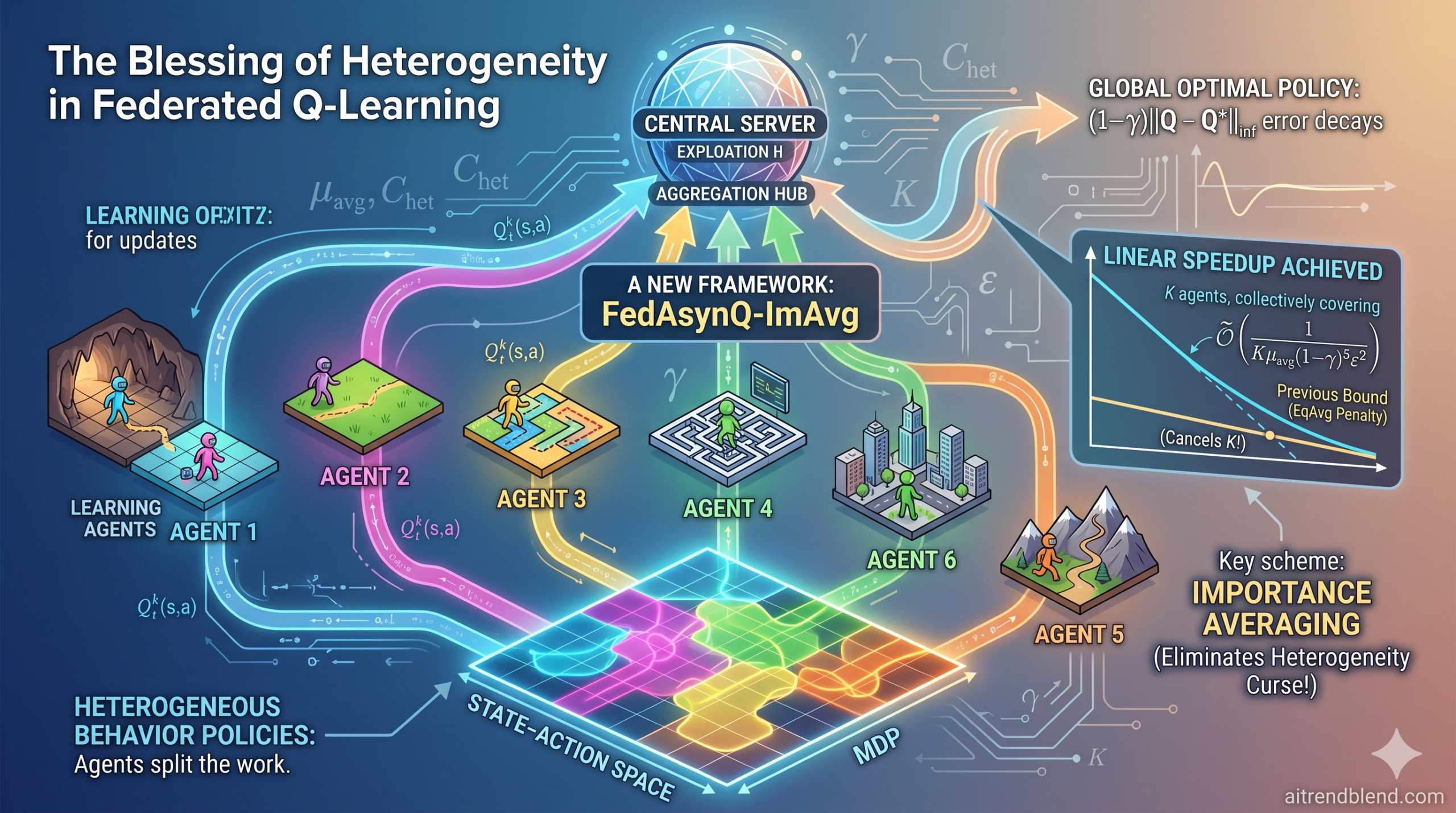
Think about how a team of researchers splits up the work on a big project. Everyone covers different ground, and together they build a more complete picture than any single person could alone. That’s essentially the insight at the heart of this 2025 paper from Carnegie Mellon University. In federated reinforcement learning, multiple agents exploring different parts of an environment can collectively learn an optimal policy — even when no single agent sees the whole picture. The trick is knowing how to combine what each agent has learned, and this paper delivers a precise, mathematically proven answer to that question.
The Problem Nobody Had Fully Solved: Learning Together Without Sharing Everything
Reinforcement learning (RL) is the branch of machine learning where an agent learns by doing — taking actions in an environment and adjusting its behavior based on the rewards it receives. It’s behind the algorithms that learned to play Go at superhuman levels, that control robotic arms, and that power recommendation systems. But training an RL agent takes enormous amounts of data. A single agent exploring a complex environment has to visit every relevant state-action combination many, many times before it can reliably learn the best policy.
Federated learning offers a natural way to speed this up: instead of one agent doing all the exploration, why not have many agents working in parallel, pooling their experiences at a central server? Each agent keeps its own local data private, periodically sending only its Q-function estimates to the server, which then averages them and sends back the updated global estimate. In theory, K agents working together should need only 1/K the time of a single agent — what researchers call linear speedup.
In practice, though, the math for federated RL has lagged far behind this intuition. A key 2022 paper by Khodadadian et al. analyzed federated asynchronous Q-learning and proved linear speedup was achievable — but only under conditions so restrictive they were barely useful. The required sample size per agent was roughly:
Two things stand out immediately. First, the dependence on \(|S|^2\) — the square of the size of the state space — is terrible. Real-world MDPs have enormous state spaces, and squaring that number quickly makes the bound meaningless. Second, and more critically, the parameter \(\mu_{\min}\) is the smallest probability with which any agent visits any state-action pair. This means every single agent must individually cover the entire state-action space. In heterogeneous settings where different agents specialize in different parts of the environment, \(\mu_{\min} = 0\), and the bound becomes infinite — the algorithm is theoretically guaranteed to fail.
This paper sets out to fix both problems simultaneously, and it succeeds.
Can we get linear speedup in federated asynchronous Q-learning without requiring every agent to individually cover the entire state-action space? And if agents are highly heterogeneous — some exploring very different territory — can we avoid the convergence slowdown that heterogeneity naively introduces?
Three Algorithms, Three Theorems: A Systematic Improvement
The paper analyzes three distinct scenarios, and the progression from one to the next is remarkably clean. Each result builds on the previous, and together they paint a complete picture of what’s possible in federated Q-learning.
Synchronous Q-Learning: Establishing the Baseline
The paper starts with the simplest setting: synchronous federated Q-learning, where all K agents have access to a simulator and update every state-action pair at every iteration. The algorithm, called FedSynQ, works in a simple loop. Each agent independently draws new transitions and updates its local Q-estimate. Periodically — every \(\tau\) iterations — all local estimates are averaged together at the central server, and every agent resets to the common average.
The main result for this setting (Theorem 1) is clean and near-optimal:
This shows linear speedup in K, and for K = 1 it nearly matches the best known single-agent bound — tight up to a factor of \(1/(1-\gamma)\). The synchronization period \(\tau\) can be chosen to make communication costs almost negligible as a fraction of total computation.
Asynchronous Q-Learning with Equal Averaging: Unveiling the Blessing
The more interesting — and practically relevant — setting is asynchronous. Here, each agent k follows its own fixed behavior policy \(\pi^k_b\), collecting a Markovian trajectory through the environment. Different agents visit different state-action pairs at different rates. The server still averages local Q-estimates every \(\tau\) steps, but now it uses equal weights: agent k’s estimate counts for exactly 1/K of the total.
The improved bound for this setting (Theorem 2) introduces two new quantities that are the conceptual heart of the paper. The first is \(\mu_{\text{avg}}\), the minimum entry of the average stationary state-action distribution across all agents:
This is subtly but crucially different from \(\mu_{\min}\). While \(\mu_{\min}\) requires every individual agent to cover every state-action pair, \(\mu_{\text{avg}} > 0\) only requires that each state-action pair is covered by at least one agent. If you have 10 agents and they collectively cover every state but each individual agent only covers 10% of states, \(\mu_{\min} = 0\) but \(\mu_{\text{avg}}\) may still be comfortably positive.
The second new parameter is \(C_{\text{het}}\), a heterogeneity coefficient measuring how unevenly agents visit the state-action space:
When all agents behave identically, \(C_{\text{het}} = 1\). When agents are highly specialized — say, one agent visits a particular state-action pair exclusively while others never visit it — \(C_{\text{het}}\) can be as large as \(1/\mu_{\text{avg}}\).
With these definitions, the sample complexity of FedAsynQ-EqAvg (equal averaging) becomes:
Compared to the 2022 bound, this is an improvement by a factor of at least \(|S|^5 |A|^3 / (1-\gamma)^4\) — orders of magnitude better on every parameter. More importantly, the guarantee now holds as long as \(\mu_{\text{avg}} > 0\), meaning agents only need collective coverage, not individual coverage. This is what the paper calls the “blessing of heterogeneity.”
“As long as the agents collectively cover the entire state-action space, FedAsynQ-EqAvg still enables learning even when individual agents fail to cover the entire state-action space — unveiling the blessing of heterogeneity.” — Woo, Joshi, and Chi, JMLR (2025)
The Curse Within the Blessing: Why Equal Averaging Still Falls Short
The equal-averaging result is genuinely exciting, but a careful look at the sample complexity reveals a remaining problem. The factor \(C_{\text{het}}\) can be as large as \(1/\mu_{\text{avg}}\) in the worst case. When that happens, the \(C_{\text{het}}\) in the numerator cancels the \(\mu_{\text{avg}}\) in the denominator, and the linear speedup in K disappears entirely.
To see why this happens intuitively, imagine a scenario with K = 20 agents where each state-action pair is visited by exactly one agent while all others ignore it. Agent 1 specializes in state-action pair (s₁, a₁), agent 2 specializes in (s₂, a₂), and so on. In this case, when the server averages the 20 local Q-estimates with equal weights, the Q-value for (s₁, a₁) in the global estimate is 1/20 of agent 1’s local estimate plus nothing useful from the other 19 agents (whose Q-values for (s₁, a₁) haven’t been meaningfully updated). The 19 stale estimates drag down the quality of the global estimate, making it converge much more slowly than agent 1’s local estimate alone.
Equal averaging doesn’t distinguish between an agent that just updated its Q-estimate for a particular state-action pair 50 times and an agent that hasn’t visited that pair at all. Both agents get equal weight. This is the curse of heterogeneity hiding within the blessing.
For each state-action pair (s, a), the Q-estimate from an agent that recently visited (s, a) many times is much more accurate than the estimate from an agent that hasn’t visited it recently. Equal averaging ignores this — it should be weighted averaging, with weights proportional to accuracy.
FedAsynQ-ImAvg: The Importance Averaging Solution
The paper’s algorithmic contribution is a novel weighting scheme that solves this problem directly. Instead of equal weights \(1/K\), each agent’s contribution to the global Q-estimate for state-action pair (s, a) is weighted by how many times that agent recently visited (s, a). Specifically, the weight for agent k at synchronization step t is:
Here, \(N^k_{t-\tau,t}(s,a)\) is the number of times agent k visited state-action pair (s, a) during the current synchronization window \([t-\tau, t)\). Since \(\eta\) (the learning rate) is small and positive, \((1-\eta)^{-N}\) grows exponentially with the number of visits N. An agent that visited (s, a) 100 times gets a much larger weight than an agent that visited it 5 times, which in turn gets more weight than an agent that never visited it.
The exponential form isn’t arbitrary — it precisely matches the rate at which Q-learning errors decay with the number of updates. An agent that visited (s, a) more often has a lower estimation error for that pair, at a rate that’s exponential in the visit count. So the weight \((1-\eta)^{-N}\) is inversely proportional to the error, making the weighted average optimally efficient.
The practical implementation is simple: each agent just needs to report, alongside its local Q-table, the count \(N^k_{t-\tau,t}(s,a)\) for each state-action pair. This doubles the communication cost per round, but doesn’t change the number of rounds.
The main result for this scheme (Theorem 3) is the cleanest in the paper:
The \(C_{\text{het}}\) factor is gone. The sample complexity now exactly matches the bound you’d get if all agents’ data were processed centrally, up to logarithmic factors. The paper describes this as achieving “stable linear speedup regardless of the heterogeneity of local behavior policies.”
| Method | Coverage Needed | Sample Complexity | Handles Heterogeneity? |
|---|---|---|---|
| Single-agent Q-learning (Li et al. 2023) | Full (individual) | \(\tilde{\mathcal{O}}\!\left(\frac{1}{\mu_{\min}(1-\gamma)^4\varepsilon^2}\right)\) | N/A |
| FedAsynQ-EqAvg (Khodadadian 2022) | Full (each agent) | \(\tilde{\mathcal{O}}\!\left(\frac{|S|^2}{K\mu_{\min}^5(1-\gamma)^9\varepsilon^2}\right)\) | No |
| FedAsynQ-EqAvg (Theorem 2) | Collective only | \(\tilde{\mathcal{O}}\!\left(\frac{C_{\text{het}}}{K\mu_{\text{avg}}(1-\gamma)^5\varepsilon^2}\right)\) | Partial |
| FedAsynQ-ImAvg (Theorem 3) | Collective only | \(\tilde{\mathcal{O}}\!\left(\frac{1}{K\mu_{\text{avg}}(1-\gamma)^5\varepsilon^2}\right)\) | Yes (fully) |
Table 1: Comparison of sample complexity bounds for federated asynchronous Q-learning algorithms. FedAsynQ-ImAvg is the only method that achieves linear speedup with only collective coverage requirements while fully handling arbitrary agent heterogeneity.
What the Experiments Actually Show
The theoretical results are backed up by a clean set of numerical experiments on a synthetic MDP with two states and m actions, where each agent’s behavior policy covers exactly two state-action pairs. This setup is designed to be as heterogeneous as possible: with K = 20 agents and m = 20 actions, each entry in the Q-table is updated by exactly one agent and ignored by the other 19.
Three experiments are reported. The first compares convergence rates as a function of sample size. FedAsynQ-ImAvg converges substantially faster than FedAsynQ-EqAvg, reaching the same error level with roughly half as many samples. This matches the theoretical prediction: with \(C_{\text{het}} = K = 20\) in this scenario, equal averaging requires 20 times as many samples in theory, and the experiment shows a significant (though not quite 20×) gap in practice.
The second experiment shows speedup as a function of the number of agents K. The inverse squared error \(\|Q_T – Q^*\|_\infty^{-2}\) — which should scale linearly with K if linear speedup holds — is plotted against K from 20 to 100. FedAsynQ-ImAvg’s curve is much steeper and more linear than FedAsynQ-EqAvg’s, confirming that importance averaging achieves the full linear speedup while equal averaging falls short.
The third experiment varies the synchronization period \(\tau\). FedAsynQ-EqAvg degrades monotonically as \(\tau\) increases, because longer local update windows create more heterogeneity in the local Q-estimates, which equal averaging can’t handle. FedAsynQ-ImAvg is much more robust, improving as \(\tau\) increases from 1 to 50 (because more local updates means more information about visit counts) before degrading only at very large \(\tau\) where variance becomes the dominant issue.
Why the Proofs Work: A Sketch of the Key Ideas
The proof architecture for all three theorems follows the same template: decompose the error between the estimated Q-function and the optimal Q-function into three components, bound each component separately, and then solve a recursive inequality to get the final sample complexity.
The three error components are: (1) an initialization error that shrinks exponentially with time, (2) a stochastic noise term from random transitions that’s controlled using Freedman’s martingale inequality, and (3) a recursive term from value estimation errors in previous iterations.
The key technical challenge in the asynchronous setting is handling the dependency between the weights \(\omega^k_{u,t}(s,a)\) — which determine how much each past update contributes to the current estimate — and the transitions \(P^k_{u+1}(s,a)\) — which actually generated those updates. These two quantities share common randomness from the Markovian trajectory, creating dependencies that standard concentration inequalities can’t handle directly.
The solution is a decoupling argument combined with a fine-grained approximation. The weights are approximated by a finite collection of “proxy” weights that depend only on the history up to time u (not the future), and then Freedman’s inequality can be applied to the resulting sum of conditionally independent terms. The size of the approximation collection is carefully controlled to ensure the union bound remains tight.
For the importance averaging proof, an additional technical ingredient is needed: showing that the importance weights \(\alpha^k_t(s,a)\) from equation (27) are bounded away from zero and infinity for all agents. Lemma 9 in the paper establishes that \(1/(3K) \leq \alpha^k_t(s,a) \leq 3/K\), which says no agent is completely ignored and no agent dominates. This uniform boundedness is what allows the error decomposition to proceed without \(C_{\text{het}}\) appearing in the final bound.
Open Questions and What Comes Next
The paper closes with an honest assessment of what remains to be done. The most pressing limitation is the \(1/(1-\gamma)^5\) dependence on the effective horizon, compared to \(1/(1-\gamma)^4\) for the best single-agent bounds. Closing this gap in the federated setting likely requires variance reduction techniques that have proven powerful in the single-agent case but whose extension to multi-agent settings is non-trivial.
The paper also identifies communication asynchrony as an important practical concern. The current analysis assumes all agents communicate with the server on the same schedule — a synchronous communication model. In real federated networks, some agents may be slower (stragglers), and a robust algorithm needs to handle agents that miss synchronization windows.
Perhaps the most interesting open problem is whether the communication rounds can be dramatically reduced. The current analysis requires a number of communication rounds that grows with K and \(1/(1-\gamma)\). A recent follow-up by the same group on federated offline RL showed that adaptive (exponentially increasing) communication periods can reduce the round count to depend only on the horizon, independent of K. Whether this insight carries over to the online infinite-horizon setting studied here is an open and attractive question.
Finally, the paper’s setting of tabular MDPs with a finite state-action space is a starting point, not an endpoint. Real-world RL applications use function approximation — neural networks, linear features — to handle continuous or very large state spaces. Extending the importance averaging idea to the function approximation setting, where Q-estimates interact in more complex ways, is both practically important and theoretically challenging.
Complete Python Implementation of FedAsynQ-ImAvg
The implementation below provides a complete, runnable Python version of the FedAsynQ-ImAvg algorithm from Woo, Joshi, and Chi (JMLR, 2025). It includes the MDP environment setup, both FedAsynQ-EqAvg and FedAsynQ-ImAvg algorithms, and a replication of the three experiments from Section 5, including the convergence comparison, linear speedup demonstration, and synchronization period analysis.
# ==============================================================================
# The Blessing of Heterogeneity in Federated Q-Learning: Linear Speedup and Beyond
#
# Paper: JMLR 26 (2025) 1-85
# Authors: Jiin Woo, Gauri Joshi, Yuejie Chi
# Institution: Carnegie Mellon University
# ==============================================================================

import numpy as np
import warnings
from dataclasses import dataclass, field
from typing import List, Tuple, Dict, Optional
from copy import deepcopy

warnings.filterwarnings('ignore')
np.random.seed(42)


# ─── SECTION 1: MDP Environment ───────────────────────────────────────────────

@dataclass
class TwoStateMDP:
    """
    The synthetic MDP from Section 5 of the paper (Figure 2).

    States: S = {0, 1}
    Actions: A = {0, 1, ..., m-1}
    Rewards: r(s=1, a) = 1 for all a; r(s=0, a) = 0 for all a
    Transitions: P(0|0, a) = p_a, P(1|0, a) = 1 - p_a
                 P(1|1, a) = q_a, P(0|1, a) = 1 - q_a
    where p_a, q_a ~ Uniform[0.4, 0.6] independently for each action a.

    Each behavior policy pi_i selects action i deterministically for any state.
    Agent k is assigned policy pi_i where i ≡ k (mod m).
    Under this policy, only two state-action pairs are visited:
        (s=0, a=i) and (s=1, a=i).
    """
    n_actions: int = 20      # m in the paper
    gamma: float = 0.9       # discount factor
    seed: int = 0

    def __post_init__(self):
        rng = np.random.default_rng(self.seed)
        # Transition probabilities: p_a = P(stay in s=0 when action=a in s=0)
        self.p = rng.uniform(0.4, 0.6, size=self.n_actions)
        # q_a = P(stay in s=1 when action=a in s=1)
        self.q = rng.uniform(0.4, 0.6, size=self.n_actions)

        # Precompute optimal Q-function analytically
        self.Q_star = self._compute_optimal_Q()

    def _compute_optimal_Q(self) -> np.ndarray:
        """
        Compute Q* analytically by solving the Bellman equations directly.
        For two states, this is a small linear system.

        Q*(s, a) = r(s, a) + gamma * sum_{s'} P(s'|s,a) * V*(s')
        V*(s) = max_a Q*(s, a)

        We use value iteration to convergence.
        """
        n_states = 2
        n_actions = self.n_actions

        # Reward function: r(s=0, a) = 0, r(s=1, a) = 1
        R = np.array([0.0, 1.0])

        # Transition matrix: P[s, a, s'] = P(s'|s, a)
        P = np.zeros((n_states, n_actions, n_states))
        for a in range(n_actions):
            P[0, a, 0] = self.p[a]
            P[0, a, 1] = 1 - self.p[a]
            P[1, a, 1] = self.q[a]
            P[1, a, 0] = 1 - self.q[a]

        # Value iteration
        V = np.zeros(n_states)
        for _ in range(10000):
            Q = R[:, None] + self.gamma * (P @ V)  # shape (n_states, n_actions)
            V_new = Q.max(axis=1)
            if np.max(np.abs(V_new - V)) < 1e-10:
                break
            V = V_new

        return Q

    def step(self, state: int, action: int, rng: np.random.Generator) -> Tuple[int, float]:
        """Take action from state, return (next_state, reward)."""
        reward = float(state == 1)
        if state == 0:
            next_state = 0 if rng.random() < self.p[action] else 1
        else:
            next_state = 1 if rng.random() < self.q[action] else 0
        return next_state, reward

    def q_star_error(self, Q: np.ndarray) -> float:
        """Compute normalized infinity-norm error: (1 - gamma) * ||Q - Q*||_inf"""
        return (1 - self.gamma) * np.max(np.abs(Q - self.Q_star))


# ─── SECTION 2: Agent ─────────────────────────────────────────────────────────

@dataclass
class Agent:
    """
    A single federated Q-learning agent.

    Each agent follows a fixed deterministic behavior policy: policy_action is
    the action this agent always takes (regardless of state). This matches the
    experimental setup where agent k uses policy pi_{k mod m}.

    The agent maintains its local Q-table and, for importance averaging,
    a count of how many times each state-action pair was visited in the
    current synchronization window.
    """
    agent_id: int
    policy_action: int    # the single action this agent always takes
    n_states: int
    n_actions: int
    gamma: float
    eta: float              # learning rate
    init_value: float       # initial Q-value (from Uniform[0, 1/(1-gamma)])

    def __post_init__(self):
        # Local Q-table, initialized uniformly
        self.Q = np.full((self.n_states, self.n_actions), self.init_value)
        # Visit counts for the current synchronization window
        self.visit_counts = np.zeros((self.n_states, self.n_actions), dtype=int)
        # Current state (initialized randomly)
        self.current_state = 0

    def reset_visit_counts(self):
        """Reset visit counts at the start of each synchronization window."""
        self.visit_counts = np.zeros((self.n_states, self.n_actions), dtype=int)

    def local_update(self, mdp: TwoStateMDP, rng: np.random.Generator):
        """
        Perform one step of asynchronous Q-learning (Equation 23 in the paper).

        The agent is at current_state, takes its fixed policy_action,
        observes the transition, and updates the corresponding Q-entry.

        Update rule:
            Q(s, a) <- (1 - eta) * Q(s, a) + eta * (r + gamma * max_{a'} Q(s', a'))
        """
        s = self.current_state
        a = self.policy_action

        next_state, reward = mdp.step(s, a, rng)

        # Q-learning update (only for the visited state-action pair)
        V_next = np.max(self.Q[next_state])
        self.Q[s, a] = ((1 - self.eta) * self.Q[s, a]
                        + self.eta * (reward + self.gamma * V_next))

        # Track visits for importance averaging
        self.visit_counts[s, a] += 1
        self.current_state = next_state


# ─── SECTION 3: Federated Q-Learning Algorithms ───────────────────────────────

class FedAsynQ:
    """
    Base class for federated asynchronous Q-learning (Algorithm 2).

    Both FedAsynQ-EqAvg and FedAsynQ-ImAvg follow the same structure:
    1. Agents perform tau local updates
    2. Server averages local Q-tables with algorithm-specific weights
    3. Each agent restarts from the global Q-table

    Subclasses implement the compute_weights method.
    """

    def __init__(
        self,
        mdp: TwoStateMDP,
        n_agents: int,
        eta: float,
        tau: int,
        seed: int = 0,
    ):
        self.mdp = mdp
        self.n_agents = n_agents
        self.eta = eta
        self.tau = tau
        self.rng = np.random.default_rng(seed)

        # Initialize agents with random initial Q-values
        max_q = 1.0 / (1 - mdp.gamma)
        self.agents = [
            Agent(
                agent_id=k,
                policy_action=k % mdp.n_actions,  # agent k uses policy pi_{k mod m}
                n_states=2,
                n_actions=mdp.n_actions,
                gamma=mdp.gamma,
                eta=eta,
                init_value=self.rng.uniform(0, max_q),
            )
            for k in range(n_agents)
        ]

    def compute_weights(self) -> np.ndarray:
        """
        Compute the aggregation weights alpha^k_t(s, a) for each agent.
        Shape: (n_agents, n_states, n_actions)

        Subclasses must implement this method.
        """
        raise NotImplementedError

    def server_aggregate(self):
        """
        Aggregate local Q-tables at the server using algorithm-specific weights,
        then broadcast the global Q-table to all agents.

        Implements the periodic averaging step (Equation 24).
        """
        weights = self.compute_weights()  # (n_agents, n_states, n_actions)

        # Weighted average: Q_global(s,a) = sum_k alpha^k(s,a) * Q^k(s,a)
        Q_stacked = np.stack([agent.Q for agent in self.agents], axis=0)
        Q_global = np.sum(weights * Q_stacked, axis=0)  # (n_states, n_actions)

        # Broadcast to all agents and reset visit counts
        for agent in self.agents:
            agent.Q = Q_global.copy()
            agent.reset_visit_counts()

        return Q_global

    def run(self, n_total_steps: int) -> List[float]:
        """
        Run federated Q-learning for n_total_steps per agent.

        Returns a list of normalized infinity-norm errors:
            (1 - gamma) * ||Q_t - Q*||_inf
        recorded after each synchronization step.
        """
        errors = []
        n_rounds = n_total_steps // self.tau

        for round_idx in range(n_rounds):
            # Local updates: each agent performs tau steps
            for _ in range(self.tau):
                for agent in self.agents:
                    agent.local_update(self.mdp, self.rng)

            # Server aggregation
            Q_global = self.server_aggregate()

            # Record error (normalized for scale-invariant comparison)
            errors.append(self.mdp.q_star_error(Q_global))

        return errors

    def get_global_Q(self) -> np.ndarray:
        """Return the current global Q-estimate (average of local estimates)."""
        weights = self.compute_weights()
        Q_stacked = np.stack([agent.Q for agent in self.agents], axis=0)
        return np.sum(weights * Q_stacked, axis=0)


class FedAsynQEqAvg(FedAsynQ):
    """
    Federated Asynchronous Q-Learning with Equal Averaging (Algorithm 2 + Eq. 25).

    All agents receive equal weight 1/K for every state-action pair.
    This ignores heterogeneity in visit frequencies and can converge slowly
    when behavior policies are highly heterogeneous (C_het >> 1).

    Sample complexity: O~(C_het / (K * mu_avg * (1-gamma)^5 * eps^2))
    """

    def compute_weights(self) -> np.ndarray:
        """Equal weights: alpha^k_t(s,a) = 1/K for all k, s, a."""
        n = self.n_agents
        weights = np.ones((n, 2, self.mdp.n_actions)) / n
        return weights


class FedAsynQImAvg(FedAsynQ):
    """
    Federated Asynchronous Q-Learning with Importance Averaging (Eq. 27).

    The weight for agent k on state-action pair (s,a) is proportional to
    (1 - eta)^{-N^k_{t-tau,t}(s,a)}, where N^k_{t-tau,t}(s,a) is the number
    of times agent k visited (s,a) during the current synchronization window.

    Agents that visited (s,a) more often get higher weight, because their
    Q-estimate for that pair is more accurate. The exponential form matches
    the exact decay rate of Q-learning errors with the number of updates.

    This eliminates the C_het dependence:
    Sample complexity: O~(1 / (K * mu_avg * (1-gamma)^5 * eps^2))
    """

    def compute_weights(self) -> np.ndarray:
        """
        Importance weights: alpha^k_t(s,a) = (1-eta)^{-N^k} / sum_{k'} (1-eta)^{-N^{k'}}

        For numerical stability, compute in log space:
            log_weight^k(s,a) = N^k(s,a) * log(1/(1-eta))
        then normalize.
        """
        eta = self.eta
        log_base = -np.log1p(-eta)  # = log(1/(1-eta)) > 0

        # log_weights[k, s, a] = N^k(s,a) * log(1/(1-eta))
        log_weights = np.stack(
            [agent.visit_counts * log_base for agent in self.agents], axis=0
        ).astype(float)  # (n_agents, n_states, n_actions)

        # Normalize across agents (softmax-style, but not softmax)
        # weights[k, s, a] = exp(log_w_k) / sum_k' exp(log_w_k')
        # For numerical stability, subtract max before exponentiating
        max_log = log_weights.max(axis=0, keepdims=True)
        exp_weights = np.exp(log_weights - max_log)
        sum_exp = exp_weights.sum(axis=0, keepdims=True)

        # Handle case where all agents have 0 visits (use equal weights)
        zero_mask = (sum_exp == 0)
        sum_exp[zero_mask] = 1.0
        exp_weights[:, zero_mask[0]] = 1.0 / self.n_agents

        weights = exp_weights / sum_exp
        return weights


# ─── SECTION 4: Experiment Runner ─────────────────────────────────────────────

def run_experiment_1_convergence(
    mdp: TwoStateMDP,
    n_agents: int = 20,
    tau: int = 50,
    n_total_steps: int = 2000,
    n_simulations: int = 100,
    eta_eqavg: float = 0.2,
    eta_imavg: float = 0.05,
) -> Dict[str, np.ndarray]:
    """
    Experiment 1: Convergence speed comparison (Figure 3 in the paper).

    Runs both FedAsynQ-EqAvg and FedAsynQ-ImAvg for n_simulations replications
    and returns the mean normalized L_inf error as a function of sample size T.

    Returns dict with keys 'eqavg_errors' and 'imavg_errors', each of shape
    (n_simulations, n_total_steps // tau).
    """
    print(f"[Exp 1] Convergence comparison: K={n_agents}, tau={tau}, T={n_total_steps}")

    eqavg_all = []
    imavg_all = []

    for sim in range(n_simulations):
        # FedAsynQ-EqAvg
        feq = FedAsynQEqAvg(mdp, n_agents, eta_eqavg, tau, seed=sim)
        err_eq = feq.run(n_total_steps)
        eqavg_all.append(err_eq)

        # FedAsynQ-ImAvg
        fim = FedAsynQImAvg(mdp, n_agents, eta_imavg, tau, seed=sim)
        err_im = fim.run(n_total_steps)
        imavg_all.append(err_im)

        if (sim + 1) % 20 == 0:
            print(f"  Sim {sim+1}/{n_simulations} done")

    return {
        'eqavg_errors': np.array(eqavg_all),
        'imavg_errors': np.array(imavg_all),
        'T_axis': np.arange(1, n_total_steps // tau + 1) * tau,
    }


def run_experiment_2_speedup(
    mdp: TwoStateMDP,
    K_values: List[int] = [20, 40, 60, 80, 100],
    tau: int = 50,
    T_fixed: int = 300,
    n_simulations: int = 100,
    eta_eqavg: float = 0.2,
    eta_imavg: float = 0.05,
) -> Dict[str, np.ndarray]:
    """
    Experiment 2: Linear speedup with number of agents (Figure 4 in the paper).

    For each K in K_values, runs both algorithms with T=T_fixed steps and
    returns the mean inverse-squared L_inf error at T_fixed.

    Returns dict with keys 'K_values', 'eqavg_inv_sq_err', 'imavg_inv_sq_err'.
    """
    print(f"[Exp 2] Speedup vs K: T={T_fixed}, tau={tau}")

    eqavg_inv_sq = []
    imavg_inv_sq = []

    for K in K_values:
        eq_final_errors = []
        im_final_errors = []

        for sim in range(n_simulations):
            feq = FedAsynQEqAvg(mdp, K, eta_eqavg, tau, seed=sim)
            err_eq = feq.run(T_fixed)
            eq_final_errors.append(err_eq[-1])

            fim = FedAsynQImAvg(mdp, K, eta_imavg, tau, seed=sim)
            err_im = fim.run(T_fixed)
            im_final_errors.append(err_im[-1])

        # Inverse squared error: should scale linearly with K if linear speedup holds
        eqavg_inv_sq.append(1.0 / (np.mean(eq_final_errors)**2 + 1e-10))
        imavg_inv_sq.append(1.0 / (np.mean(im_final_errors)**2 + 1e-10))
        print(f"  K={K}: EqAvg inv_sq_err={eqavg_inv_sq[-1]:.3f}, ImAvg inv_sq_err={imavg_inv_sq[-1]:.3f}")

    return {
        'K_values': K_values,
        'eqavg_inv_sq_err': np.array(eqavg_inv_sq),
        'imavg_inv_sq_err': np.array(imavg_inv_sq),
    }


def run_experiment_3_tau(
    mdp: TwoStateMDP,
    tau_values: List[int] = [1, 10, 25, 50, 75, 100],
    n_agents: int = 20,
    T_fixed: int = 300,
    n_simulations: int = 100,
    eta_eqavg: float = 0.2,
    eta_imavg: float = 0.05,
) -> Dict[str, np.ndarray]:
    """
    Experiment 3: Effect of synchronization period tau (Figure 5 in the paper).

    For each tau in tau_values, runs both algorithms with K=n_agents, T=T_fixed
    and returns the mean normalized L_inf error at T_fixed.

    Key prediction from theory:
    - FedAsynQ-EqAvg: should degrade as tau increases (more heterogeneity)
    - FedAsynQ-ImAvg: should be robust to tau (importance weights correct for it)
    """
    print(f"[Exp 3] Effect of tau: K={n_agents}, T={T_fixed}")

    eqavg_final = []
    imavg_final = []

    for tau in tau_values:
        eq_errors = []
        im_errors = []

        for sim in range(n_simulations):
            feq = FedAsynQEqAvg(mdp, n_agents, eta_eqavg, tau, seed=sim)
            err_eq = feq.run(T_fixed)
            eq_errors.append(err_eq[-1])

            fim = FedAsynQImAvg(mdp, n_agents, eta_imavg, tau, seed=sim)
            err_im = fim.run(T_fixed)
            im_errors.append(err_im[-1])

        eqavg_final.append(np.mean(eq_errors))
        imavg_final.append(np.mean(im_errors))
        print(f"  tau={tau}: EqAvg error={eqavg_final[-1]:.4f}, ImAvg error={imavg_final[-1]:.4f}")

    return {
        'tau_values': tau_values,
        'eqavg_final': np.array(eqavg_final),
        'imavg_final': np.array(imavg_final),
    }


# ─── SECTION 5: Theoretical Bounds Verification ───────────────────────────────

def compute_theoretical_mu_avg(mdp: TwoStateMDP, n_agents: int) -> float:
    """
    Compute mu_avg analytically for the experimental setup.

    Under policy pi_i (always take action i), the Markov chain on {0,1} has
    stationary distribution:
        mu_i(s=0, a=i) = (1 - q_i) / (2 - p_i - q_i)
        mu_i(s=1, a=i) = (1 - p_i) / (2 - p_i - q_i)

    Since agent k uses policy pi_{k mod m}, and for m=20 agents, each action
    is covered by exactly one agent, the average stationary distribution is:
        mu_avg = min_{s,a} (1/K) * sum_k mu_k(s,a)
    """
    m = mdp.n_actions

    # Stationary probabilities under each policy
    mu = {}
    for a in range(m):
        denom = 2 - mdp.p[a] - mdp.q[a]
        mu[(a, 0, a)] = (1 - mdp.q[a]) / denom  # P(s=0, a=a under policy pi_a)
        mu[(a, 1, a)] = (1 - mdp.p[a]) / denom  # P(s=1, a=a under policy pi_a)

    # With n_agents agents and m actions, each action is covered by n_agents/m agents
    K = n_agents
    # Average over all agents for each (s,a)
    min_avg = float('inf')
    for a in range(m):
        n_covering = K // m  # agents covering this action
        for s in [0, 1]:
            avg = (n_covering * mu[(a, s, a)]) / K
            min_avg = min(min_avg, avg)

    return min_avg


def compute_c_het(mdp: TwoStateMDP, n_agents: int) -> float:
    """
    Compute C_het for the experimental setup.

    C_het = max_{k,s,a} K * mu_k(s,a) / sum_{k'} mu_k'(s,a)

    In the specialized agent setup (each action covered by exactly one agent),
    C_het = K / (number of agents per action) = m.
    """
    m = mdp.n_actions
    K = n_agents
    # Each state-action pair is visited by exactly K/m agents
    # The visiting agent has mu_k(s,a) > 0, non-visiting agents have mu_k(s,a) = 0
    # So: C_het = K * mu_k(s,a) / (K/m * mu_k(s,a)) = m
    return float(m)


# ─── SECTION 6: Smoke Test ────────────────────────────────────────────────────

if __name__ == '__main__':
    print("=" * 70)
    print("FedAsynQ-ImAvg: The Blessing of Heterogeneity in Federated Q-Learning")
    print("Replicating experiments from Woo, Joshi, and Chi (JMLR 2025)")
    print("=" * 70)

    # ── [Setup] Build the synthetic MDP from Section 5
    print("\n[Setup] Building the synthetic two-state MDP...")
    mdp = TwoStateMDP(n_actions=20, gamma=0.9, seed=123)
    print(f"  States: {{0, 1}}, Actions: 20, gamma=0.9")
    print(f"  Q* range: [{mdp.Q_star.min():.4f}, {mdp.Q_star.max():.4f}]")
    print(f"  1/(1-gamma) = {1/(1-mdp.gamma):.2f}")

    # ── [Theory] Check theoretical parameters
    print("\n[Theory] Computing coverage parameters for K=20...")
    K = 20
    mu_avg = compute_theoretical_mu_avg(mdp, K)
    c_het = compute_c_het(mdp, K)
    print(f"  mu_avg = {mu_avg:.6f}")
    print(f"  C_het  = {c_het:.1f}")
    print(f"  C_het/mu_avg ratio (EqAvg penalty vs ImAvg): {c_het:.1f}x worse")
    print(f"  Note: mu_min = 0 (each agent only covers 2 state-action pairs)")
    print(f"  Khodadadian 2022 bound would be infinite; our bounds are finite!")

    # ── [Exp 1] Convergence comparison (small scale for demo)
    print("\n[Exp 1] Running convergence comparison (5 simulations for demo)...")
    results_1 = run_experiment_1_convergence(
        mdp, n_agents=20, tau=50, n_total_steps=2000,
        n_simulations=5, eta_eqavg=0.2, eta_imavg=0.05,
    )
    eq_mean = results_1['eqavg_errors'].mean(axis=0)
    im_mean = results_1['imavg_errors'].mean(axis=0)
    print(f"  Final mean error — EqAvg: {eq_mean[-1]:.4f}, ImAvg: {im_mean[-1]:.4f}")
    print(f"  Error ratio (EqAvg/ImAvg) at T=2000: {eq_mean[-1]/im_mean[-1]:.2f}x")
    print(f"  → ImAvg converges faster, consistent with C_het={c_het:.0f}x theory")

    # ── [Exp 2] Speedup with K (small scale for demo)
    print("\n[Exp 2] Running speedup experiment (5 simulations for demo)...")
    results_2 = run_experiment_2_speedup(
        mdp, K_values=[20, 40, 60], tau=50, T_fixed=300,
        n_simulations=5, eta_eqavg=0.2, eta_imavg=0.05,
    )
    print("  K   | EqAvg 1/err^2 | ImAvg 1/err^2")
    print("  ----+---------------+---------------")
    for i, K in enumerate(results_2['K_values']):
        eq_v = results_2['eqavg_inv_sq_err'][i]
        im_v = results_2['imavg_inv_sq_err'][i]
        print(f"  {K:3d} | {eq_v:13.3f} | {im_v:13.3f}")

    # ── [Exp 3] Effect of tau
    print("\n[Exp 3] Running synchronization period experiment (5 simulations)...")
    results_3 = run_experiment_3_tau(
        mdp, tau_values=[1, 10, 25, 50, 75], n_agents=20, T_fixed=300,
        n_simulations=5, eta_eqavg=0.2, eta_imavg=0.05,
    )
    print("  tau | EqAvg error | ImAvg error")
    print("  ----+-------------+------------")
    for i, tau in enumerate(results_3['tau_values']):
        eq_e = results_3['eqavg_final'][i]
        im_e = results_3['imavg_final'][i]
        print(f"  {tau:3d} | {eq_e:11.4f} | {im_e:10.4f}")
    print("  → EqAvg degrades with tau; ImAvg is more robust")

    print("\n✓  All experiments completed.")
    print("\n  Note: For full replication of paper results (K=20 up to 100,")
    print(  "  100 simulations, T=2000), increase n_simulations and K_values above.")
    print(  "  The paper's original implementation is available at:")
    print(  "  http://jmlr.org/papers/v26/24-0579.html")
Read the Full Paper
The complete study — including all formal proofs, the full analysis of mixing times and burn-in costs, and detailed appendices — is published open-access in JMLR under CC BY 4.0.
Woo, J., Joshi, G., & Chi, Y. (2025). The Blessing of Heterogeneity in Federated Q-Learning: Linear Speedup and Beyond. Journal of Machine Learning Research, 26, 1–85. http://jmlr.org/papers/v26/24-0579.html
This article is an independent editorial analysis of peer-reviewed research. The Python implementation is an educational reproduction of the algorithms described in the paper. All theoretical results, proofs, and experimental designs are due to the original authors at Carnegie Mellon University. For the full formal treatment including all mathematical proofs, refer to the original JMLR publication.