Key Points
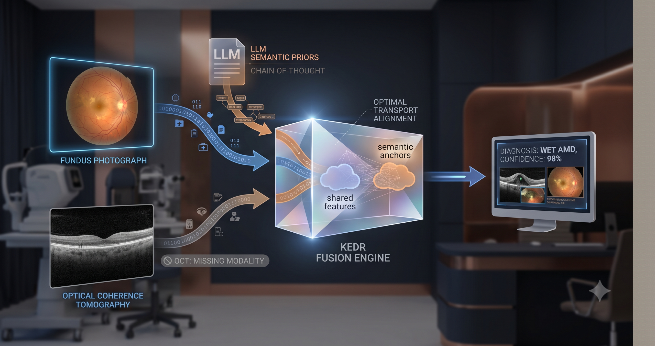
- KEDR addresses the missing-modality problem in multimodal medical imaging without reconstructing absent scans — it instead extracts shared disease semantics from GPT-4 using Chain-of-Thought prompting and anchors learned features to those semantics via optimal transport.
- A Confidence-aware Adaptive Deep Fusion module scores each modality’s reliability from its prediction error and iteratively refines the fused representation using deep equilibrium theory until the output stabilises.
- On three public datasets covering AMD, glaucoma, and skin cancer, KEDR outperforms seven state-of-the-art missing-modality baselines at 20, 40, 60, and 80 percent missing rates.
- The method’s inference cost is comparable to a baseline with 91M parameters despite KEDR training with roughly 230M, because the text encoder and confidence networks are removed at test time.
- The framework is currently limited to two-modality settings and has not been validated on real clinical missing-data distributions where patterns are irregular rather than randomly sampled.
Why Implicit Disentanglement Is Not Enough
The standard approach to missing-modality robustness is disentanglement. The idea is straightforward enough: if you can train a model to separate what two modalities share from what each one contributes uniquely, then losing one modality does not destroy the shared information. The shared branch carries what both scans would have agreed on, and the model can still predict from that.
The problem is how that shared branch is defined in practice. Most existing methods, including the ones KEDR competes against, learn shared features implicitly. They impose statistical constraints — orthogonality losses, mutual information bounds, contrastive objectives — that push the shared and specific branches apart in a latent space. The word “implicit” here matters. There is no external reference telling the model what a shared disease feature actually means. The model finds a separation that satisfies the mathematical constraint, but nothing guarantees that the resulting “shared” vector captures anything clinically meaningful. It might pick up scanner artifacts that happen to be consistent across both modalities. It might collapse to a representation that is statistically orthogonal to the modality-specific features but semantically empty.
The authors make a pointed observation about this. When modality data is scarce — which is precisely the regime they care about — implicit separation is especially unstable. There is simply not enough signal to push the latent distributions apart reliably. The paper cites prior work showing that such methods suffer systematic performance degradation once the missing rate exceeds moderate levels. The class-wise breakdown in their experiments confirms the pattern: methods that seemed competitive at 20 percent missing rate collapse at 60 and 80 percent.
There is a second, quieter failure mode. Most multimodal fusion methods weight all modalities equally at decision time. This is a simplifying assumption that feels safe but frequently is not. Diagnosing wet AMD depends more heavily on OCT than fundus imaging, because the key lesion — subretinal fluid — is visible in cross-section but hard to read from above. If the model treats both channels as equally reliable, it will average away exactly the signal that matters most in that disease category. KEDR addresses both problems separately and then combines the solutions.
The Two Ideas That Drive KEDR
The paper introduces two modules that work in sequence. The first is called Knowledge-enhanced Explicit Disentanglement, or KED. The second is the Confidence-aware Adaptive Deep Fusion module, or CAD. They are not independently novel in every component — optimal transport has been applied to cross-modal alignment before, and deep equilibrium models have been used in fusion before — but the specific combination, applied to the missing-modality medical imaging problem, is new.
KED: Giving the Shared Branch a Semantic Target
The central idea in KED is simple enough to state in one sentence. Rather than letting the model discover what “shared” means from data alone, you tell it what shared looks like by asking a language model that already knows the disease.
The authors use GPT-4 with a carefully constructed Chain-of-Thought prompt. A naive prompt — “what features distinguish wet AMD?” — produces exactly what you would expect from a general-purpose language model asked to describe a disease: a mix of visually observable attributes and clinical symptoms that are not visible in any image, like pain or visual blur. Figure 3 in the paper colour-codes the output, and the problem is clear. Roughly half the highlighted text corresponds to symptoms a model could never see in a scan.
The CoT prompt fixes this in two steps. The first step instructs GPT-4 to take the role of a medical imaging expert and describe only the visual and structural characteristics that are consistently reflected across multiple imaging modalities. It is told explicitly not to describe findings specific to one modality and not to describe clinical symptoms. The second step then asks it to compress those descriptions into a structured semantic prior — a compact set of cross-modal disease attributes that characterise the category for the purpose of multimodal feature alignment. The result is not a generic description of the disease but a distillation of what fundus imaging and OCT should agree on when they both show the same condition.
That structured description is then encoded using BioClinicalBERT, which has been pre-trained on clinical text and produces richer medical embeddings than a general-purpose encoder would. A linear projection maps it to the same 2048-dimensional space as the image features.
The alignment step uses optimal transport. The intuition behind OT is that it finds the most efficient way to move one distribution of mass to match another. In this context, the “source” is the distribution of shared features the model has learned so far, and the “target” is the distribution of semantic prior embeddings. The transport plan defines how much of each shared feature should be aligned to each semantic anchor. Unlike a simple MSE or cosine similarity loss, OT is sensitive to the geometry of the feature space and is robust to distributional mismatch between the two sides.
The specific formulation uses entropic regularisation, which produces a soft transport plan rather than a hard matching. This is important. Hard matching would force each shared feature vector to map to exactly one semantic anchor, which would destroy intra-class diversity — different patients with the same diagnosis should still have different features. The soft plan allows each feature to align partially with multiple semantic anchors, preserving variation while still pulling the shared representation toward clinically meaningful structure.
The OT loss is combined with an orthogonality constraint between the shared branch and each modality-specific branch. Orthogonality ensures the specific branches are not just duplicating what the shared branch already captures.
OT alignment — entropic-regularised optimal transport
$$\mathbf{T}^* = \mathrm{argmin}_{\mathbf{T} \geq 0} \langle \mathbf{C}, \mathbf{T} \rangle – \epsilon H(\mathbf{T})$$where C is the pairwise Euclidean cost matrix between semantic prior embeddings and shared features, H(T) is the entropy of the transport plan, and ε is the regularisation coefficient. The OT loss is then the sum of element-wise products between the plan and the cost matrix.
The two-step CoT prompt forces GPT-4 to output only visually grounded, cross-modal attributes — not general clinical descriptions. The difference shows up in the ablation: removing the second CoT step drops F1 by about one percentage point, and removing CoT entirely drops it by roughly three points on MMC-AMD.
CAD: Treating Modality Reliability as a Learnable Signal
After KED has produced a shared feature and two modality-specific features, the question becomes how to combine them. The simplest approaches — concatenation, averaging — assume all three sources are equally trustworthy. That assumption breaks down the moment one modality is absent or degraded.
The CAD module estimates a reliability score for each branch and uses that score to gate the features before fusion. The reliability criterion comes from a concept called true class probability, or TCP. The idea is that a model which assigns high probability to the correct class on modality-specific features from that modality is reliably encoding the disease signal. A model that spreads its probability mass widely, or assigns low probability to the correct class, is uncertain. During training, the model learns a small regression network that predicts this TCP value from the features alone, so that at test time — when ground truth labels are unavailable — it can still estimate confidence without knowing the answer.
The fusion itself is formulated as a fixed-point problem. Instead of passing the confidence-weighted features through a single feedforward network and reading off the output, KEDR defines a fusion operator and solves for the representation at which the operator applied to itself produces no further change. This is the deep equilibrium formulation. In practice it means iterating Broyden’s method — a quasi-Newton solver — until the fused vector converges. The practical effect is that cross-modal information has time to propagate through repeated refinement steps rather than a single pass, and inconsistencies between modalities tend to wash out as the representation stabilises.
The shared representation maintained the highest and most concentrated confidence distribution, typically peaking near 0.98 to 1.00, even as individual modality branches showed mixed or degraded confidence when their modality was absent. Observed in KEDR confidence density analysis, MMC-AMD dataset
The visualisations of confidence density in the paper are genuinely informative. When OCT is missing, the OCT branch’s confidence distribution flattens and shifts toward lower values. The fundus branch and the shared branch increase in confidence, compensating for the absent signal. When fundus is missing, the roles reverse. The shared representation stays high across all conditions, which is exactly what you want from a branch trained to capture what both modalities agree on.
Experimental Results, Honestly Read
The paper tests KEDR on three datasets. MMC-AMD covers four AMD categories (wet AMD, dry AMD, PCV, and normal) using fundus photography and OCT, with 615 training pairs and 153 test pairs. Harvard30k Glaucoma covers normal and glaucoma using the same two imaging modalities, with 1487 training pairs and 372 test pairs. Derm7pt covers five skin lesion categories using clinical and dermoscopic images, with 413 training pairs and 395 test pairs. All three have been used in prior missing-modality work, which makes comparison reliable.
The evaluation runs at four missing rates — 20, 40, 60, and 80 percent — and reports F1 score, Cohen’s Kappa, and accuracy. Seven competing methods are included, ranging from straightforward modality dropout through knowledge distillation approaches, shared-specific feature learning, and the most recent multi-optimal-transport and deep-equilibrium baselines from 2024 and 2025.
| Method | 20% missing | 40% missing | 60% missing | 80% missing |
|---|---|---|---|---|
| ShaSpec (CVPR 2023) | 85.01 / 75.93 / 83.66 | 81.73 / 74.78 / 83.01 | 80.60 / 72.12 / 81.05 | 78.98 / 69.82 / 79.74 |
| MoMKE (ACM MM 2024) | 80.63 / 75.35 / 83.66 | 80.91 / 76.45 / 84.31 | 81.88 / 75.05 / 83.01 | 77.92 / 71.64 / 80.39 |
| IMDR (AAAI 2025) | 83.22 / 76.38 / 84.31 | 81.32 / 73.31 / 82.35 | 80.70 / 73.53 / 82.35 | 79.09 / 73.47 / 82.35 |
| KEDR (this paper) | 85.02 / 77.38 / 84.97 | 83.34 / 78.50 / 85.62 | 83.81 / 76.93 / 84.31 | 80.81 / 73.82 / 82.35 |
The numbers are consistent across datasets and metrics, which is the most credible kind of result in this field. KEDR is not trading F1 for Kappa or performing well on one dataset while degrading on another. What stands out most is the behaviour at 60 and 80 percent missing. Competing methods tend to drop sharply once missingness exceeds 40 percent. KEDR’s curves in Figure 5 and Figure 10 of the paper are noticeably flatter. By 80 percent missing on MMC-AMD, KEDR still achieves 80.81 F1 against the next best 79.09 from IMDR — a modest absolute gap, but one that holds across all three datasets.
The glaucoma dataset shows the same pattern with starker numbers. At 20 percent missing, KEDR improves F1 from 73.46 to 74.16 over the best baseline. At 80 percent, the gap widens to over a full point in F1 and nearly five points in Kappa. On Derm7pt the Kappa improvement at 20 percent missing is more than five points over the best baseline — a large gap that the authors do not oversell but that seems genuine given how consistently it holds across missing rates.
The calibration results in Table 3 of the paper deserve specific attention. Expected calibration error measures how well a model’s stated confidence matches its actual accuracy. KEDR achieves the lowest ECE at all four missing rates on MMC-AMD, reaching 0.125 at 20 percent missing and 0.173 at 80 percent, compared to the next best competitor at 0.133 and 0.345. That is a large gap at 80 percent missing, and it matters clinically: a model that knows when it is uncertain is safer to deploy than one that is confidently wrong.
KEDR’s Expected Calibration Error at 80 percent missing rate is roughly half that of the next best method. In a clinical setting where trust in an AI output matters as much as raw accuracy, calibration is not a secondary metric — it is arguably the primary one.
What the Ablation Actually Tells You
The ablation study removes one component at a time and measures the performance drop. A few results stand out beyond the obvious conclusion that all three components contribute.
Removing the OT alignment (the “w/o OT” condition) while keeping KED’s orthogonality loss produces a smaller drop than removing the entire KED module. On MMC-AMD at 20 percent missing, KED removal costs about 3 F1 points, while OT removal alone costs about 2.5. This tells you that the semantic priors matter and the geometric alignment matters, but they are not equally important — the cross-modal structure of the shared encoder contributes even without explicit OT guidance. Replacing OT with a contrastive alignment loss produces a small but consistent degradation, which suggests the soft transport plan is doing something a pairwise similarity objective cannot replicate.
The fine-grained ablation of the CAD module is also interesting. When you remove confidence weighting but keep the DEQ iteration, the model loses about 2.6 F1 points. When you remove DEQ but keep confidence weighting, it loses about 2.8 points. The two contributions are roughly additive, which means neither dominates — you genuinely need both the reliability estimation and the iterative convergence.
The CoT design comparison in Table 8 is worth reading carefully. Without any CoT, F1 is 81.99 and Kappa is 75.64. Adding only the first CoT step — modality-agnostic conceptual description — jumps F1 to 83.98. Adding the second step — modality-aware semantic distillation — reaches 85.02. This two-point gain from a single prompting change is meaningful, and it suggests that the specific way you instruct the LLM to reason about cross-modal attributes is not a detail. It is load-bearing.
Clinical Translation Gap
The paper is honest about the distance between these results and a deployable diagnostic system, and it is worth being concrete about what that distance looks like.
All three datasets are small by medical imaging standards. MMC-AMD has 615 training pairs. Harvard30k Glaucoma has 1487. Derm7pt has 413. These are common benchmarks in the field, but they are far from the scale required to draw conclusions about real-world diagnostic performance. The training distribution and the missing-modality distribution may not match what a clinic actually sees.
The missing-modality simulation in the paper is random sampling — each scan is dropped with a fixed probability independently of disease category, image quality, or scanner availability. Real missing data patterns are not random. A clinic might routinely lack OCT for certain patient populations. A scanner might fail systematically for high-myopia eyes. Corruption might be correlated with the severity of the disease you are trying to detect. The paper conducts a supplementary experiment with incomplete-data training and shows that performance degrades moderately compared to complete-data training, which is reassuring, but the evaluation protocol still uses controlled random missingness at test time.
The two-modality constraint is stated explicitly as a limitation. Most real-world multimodal clinical workflows involve three or more sources — fundus, OCT, clinical metadata, patient history, and sometimes fluorescein angiography. Extending KEDR to that setting is not trivial. The KED module would need to handle higher-order shared representations across all active modalities simultaneously, and the confidence estimation framework would need to balance a larger set of reliability scores in the fusion step.
Finally, the training cost of 30.4 GFLOPs and 16 GB GPU memory is manageable for a research setup, but deploying this in a teleophthalmology workflow at scale would require optimisation work. The authors mention low-rank approximations of optimal transport and shared-parameter architectures as potential efficiency paths, but those experiments are not in the paper.
What Other Research This Connects To
The choice of optimal transport for cross-modal alignment sits in a growing literature. The RIMA baseline the authors compare against also uses multi-optimal transport, applied differently — aligning label features with image features rather than semantic priors with shared representations. The performance gap between RIMA and KEDR at high missing rates suggests the semantic prior grounding matters beyond transport alignment alone.
The deep equilibrium model for fusion draws on work by Bai, Kolter, and Koltun, and has been applied to multimodal fusion in a 2023 preprint from Ni et al. and in the ADFusion framework for cancer subtype prediction. The connection between DEQ stability and missing-modality robustness is intuitive — an iterative fixed-point solver naturally handles the fact that the input to fusion varies in quality and completeness — but KEDR is, to the best of this reading, the first to combine DEQ fusion with confidence weighting and explicit semantic disentanglement in the same pipeline.
The use of BioClinicalBERT to encode medical semantic priors connects to a broader thread in medical AI where domain-adapted language models consistently outperform general encoders on clinical text. The choice matters here because the semantic prior is the anchor for the entire disentanglement process. A noisier or less medically grounded encoding would propagate errors through the OT alignment and degrade the shared representation.
For practitioners building multimodal diagnostic systems, the paper’s most transferable insight is the two-step CoT prompting strategy. It is a prompt engineering approach that costs nothing to implement in any LLM-assisted medical AI pipeline, and the ablation evidence suggests it contributes meaningfully to downstream task performance independently of the KEDR architecture. The idea of asking the model to reason about cross-modal consistency before asking it to describe the disease category is likely to generalise well beyond ophthalmology and dermatology.
Readers building on this work may also find it useful to review our overview of AI for medical imaging [PLACEHOLDER — replace with confirmed live URL], which covers the broader landscape of diagnostic AI methods this research builds on.
A Complete PyTorch Implementation of KEDR
The following is a full, reproducible PyTorch implementation covering the shared encoder with cross-modal co-attention, the KED module with OT alignment, the CAD module with TCP confidence estimation and DEQ fusion, all loss functions matching the paper, a training loop, an evaluation function, and a runnable smoke test on dummy data.
# =============================================================
# KEDR: Knowledge-enhanced Explicit Disentangled Representation
# Full PyTorch implementation based on:
#   Li et al., Information Fusion 136 (2026) 104502
#   https://github.com/lijing-coder/KEDR
# =============================================================

import torch
import torch.nn as nn
import torch.nn.functional as F
from torch.optim import Adam
import numpy as np

# ---- Optimal Transport (Sinkhorn) ----------------------------

def sinkhorn(cost: torch.Tensor, eps: float = 0.1, max_iter: int = 50) -> torch.Tensor:
    """Entropic-regularised OT via Sinkhorn iterations.

    Args:
        cost: (N, M) pairwise cost matrix.
        eps:  Regularisation coefficient.
        max_iter: Number of Sinkhorn iterations.

    Returns:
        T: (N, M) soft transport plan.
    """
    N, M = cost.shape
    # Uniform marginals
    mu = torch.full((N,), 1.0 / N, device=cost.device)
    nu = torch.full((M,), 1.0 / M, device=cost.device)
    K = torch.exp(-cost / eps)          # Gibbs kernel
    u = torch.ones(N, device=cost.device)
    for _ in range(max_iter):
        v = nu / (K.T @ u + 1e-8)
        u = mu / (K @ v + 1e-8)
    T = torch.diag(u) @ K @ torch.diag(v)
    return T


def ot_loss(sem: torch.Tensor, shared: torch.Tensor, eps: float = 0.1) -> torch.Tensor:
    """Compute the OT alignment loss (Eq. 7 in paper)."""
    # Pairwise Euclidean cost matrix
    C = torch.cdist(sem, shared, p=2)
    T = sinkhorn(C, eps=eps)
    return (T * C).sum()


# ---- Shared Encoder (cross-modal co-attention) ---------------

class SharedEncoder(nn.Module):
    """Cross-modal co-attention encoder (Eq. 3-4 in paper)."""
    def __init__(self, d: int = 2048):
        super().__init__()
        self.phi_m1 = nn.Linear(d, d)
        self.phi_m2 = nn.Linear(d, d)
        self.fc_att  = nn.Linear(d, d)

    def forward(self, x_m1: torch.Tensor, x_m2: torch.Tensor):
        p1 = self.phi_m1(x_m1)   # (B, d)
        p2 = self.phi_m2(x_m2)
        A  = p1 * p2              # element-wise product — co-attention (Eq. 3)
        g  = torch.sigmoid(self.fc_att(A))
        fs = g * p1 + g * p2      # shared feature (Eq. 3)
        return fs


# ---- Modality-specific Encoders ------------------------------

class SpecificEncoder(nn.Module):
    def __init__(self, d: int = 2048):
        super().__init__()
        self.mlp = nn.Sequential(
            nn.Linear(d, d),
            nn.ReLU(),
            nn.Linear(d, d),
        )
    def forward(self, x: torch.Tensor):
        return self.mlp(x)


# ---- KED Module ----------------------------------------------

class KEDModule(nn.Module):
    """Knowledge-enhanced Explicit Disentanglement.

    Wraps the shared encoder and modality-specific encoders,
    computes the OT and orthogonality losses (Eqs 5-9).
    """
    def __init__(self, d: int = 2048, ot_eps: float = 0.1):
        super().__init__()
        self.shared_enc = SharedEncoder(d)
        self.enc_m1     = SpecificEncoder(d)
        self.enc_m2     = SpecificEncoder(d)
        self.ot_eps     = ot_eps

    def forward(self, x_m1, x_m2, x_sem):
        # Disentangle (Eq. 4)
        f_m1 = self.enc_m1(x_m1)
        f_m2 = self.enc_m2(x_m2)
        f_s  = self.shared_enc(x_m1, x_m2)

        # OT alignment loss (Eq. 7)
        loss_ot   = ot_loss(x_sem, f_s, eps=self.ot_eps)

        # Orthogonality loss (Eq. 8)
        orth_m1   = (f_s.T @ f_m1).norm(p=2) ** 2
        orth_m2   = (f_s.T @ f_m2).norm(p=2) ** 2
        loss_orth = orth_m1 + orth_m2

        loss_disent = loss_ot + loss_orth   # Eq. 9
        return f_m1, f_m2, f_s, loss_disent


# ---- TCP Confidence Estimator --------------------------------

class TCPEstimator(nn.Module):
    """True Class Probability estimator (Eq. 10-11)."""
    def __init__(self, d: int = 2048):
        super().__init__()
        self.net = nn.Sequential(
            nn.Linear(d, 256),
            nn.ReLU(),
            nn.Linear(256, 1),
        )
    def forward(self, h: torch.Tensor):
        return torch.sigmoid(self.net(h)).squeeze(-1)   # (B,)


# ---- DEQ Fusion Operator ------------------------------------

class DEQFusionOperator(nn.Module):
    """Fusion operator F_theta (Eq. 15).

    Takes concatenation of current fused state z and three
    disentangled features, outputs refined z.
    """
    def __init__(self, d: int = 2048):
        super().__init__()
        self.phi = nn.Sequential(
            nn.Linear(d * 4, d * 2),
            nn.ReLU(),
            nn.Linear(d * 2, d),
        )
    def forward(self, z, h_s, h_m1, h_m2):
        cat = torch.cat([z, h_s, h_m1, h_m2], dim=-1)
        return self.phi(cat)


def deq_solve(F_fn, h_s, h_m1, h_m2, max_iter=30, tol=1e-4) -> torch.Tensor:
    """Fixed-point iteration approximating Broyden's method.

    Iterates z = F(z, h_s, h_m1, h_m2) until convergence.
    In production, replace with the torch-deq or DEQ library.
    """
    z = torch.zeros_like(h_s)
    for _ in range(max_iter):
        z_new = F_fn(z, h_s, h_m1, h_m2)
        if (z_new - z).norm() < tol:
            break
        z = z_new
    return z


# ---- CAD Module ---------------------------------------------

class CADModule(nn.Module):
    """Confidence-aware Adaptive Deep Fusion (Eqs 10-15)."""
    def __init__(self, d: int = 2048):
        super().__init__()
        self.tcp_m1 = TCPEstimator(d)
        self.tcp_m2 = TCPEstimator(d)
        self.tcp_s  = TCPEstimator(d)
        self.F_theta = DEQFusionOperator(d)

    def forward(self, f_m1, f_m2, f_s):
        # Confidence scores
        c_m1 = self.tcp_m1(f_m1).unsqueeze(-1)   # (B, 1)
        c_m2 = self.tcp_m2(f_m2).unsqueeze(-1)
        c_s  = self.tcp_s(f_s).unsqueeze(-1)
        # Confidence-weighted features (Eq. 11)
        h_m1 = c_m1 * f_m1
        h_m2 = c_m2 * f_m2
        h_s  = c_s  * f_s
        # DEQ fixed-point fusion (Eqs 13-15)
        z_star = deq_solve(self.F_theta, h_s, h_m1, h_m2)
        return z_star, c_m1.squeeze(), c_m2.squeeze(), c_s.squeeze()


# ---- Full KEDR Model ----------------------------------------

class KEDR(nn.Module):
    """Full KEDR framework."""
    def __init__(self, d: int = 2048, num_classes: int = 4, ot_eps: float = 0.1):
        super().__init__()
        self.ked = KEDModule(d, ot_eps)
        self.cad = CADModule(d)
        self.classifier = nn.Linear(d, num_classes)
        # Learnable loss weights (Eq. 17), parameterised as exp(omega)
        self.log_w1 = nn.Parameter(torch.zeros(1))
        self.log_w2 = nn.Parameter(torch.zeros(1))

    def forward(self, x_m1, x_m2, x_sem):
        f_m1, f_m2, f_s, loss_disent = self.ked(x_m1, x_m2, x_sem)
        z_star, c_m1, c_m2, c_s = self.cad(f_m1, f_m2, f_s)
        logits = self.classifier(z_star)
        return logits, loss_disent, (c_m1, c_m2, c_s), (f_m1, f_m2, f_s)

    def loss(self, logits, labels, loss_disent, confidences, features):
        c_m1, c_m2, c_s = confidences
        f_m1, f_m2, f_s = features
        # Classification cross-entropy (Eq. 16)
        loss_cls = F.cross_entropy(logits, labels)
        # TCP confidence calibration loss (Eq. 12)
        # Approximate true class probability from predictions
        probs = torch.softmax(logits.detach(), dim=-1)
        one_hot = F.one_hot(labels, num_classes=logits.size(-1)).float()
        tcp_true = (one_hot * probs).sum(dim=-1)   # (B,)
        loss_conf = (
            (c_m1 - tcp_true).pow(2).mean() +
            (c_m2 - tcp_true).pow(2).mean() +
            (c_s  - tcp_true).pow(2).mean()
        ) / 3
        # Total loss with learnable weights (Eq. 17)
        w1 = self.log_w1.exp()
        w2 = self.log_w2.exp()
        total = loss_disent + w1 * loss_conf + w2 * loss_cls
        return total, loss_cls, loss_conf, loss_disent


# ---- Training Loop -------------------------------------------

def train_one_epoch(model, loader, optimiser, device):
    model.train()
    total_loss = 0.0
    for x_m1, x_m2, x_sem, labels in loader:
        x_m1, x_m2, x_sem, labels = (
            x_m1.to(device), x_m2.to(device),
            x_sem.to(device), labels.to(device)
        )
        optimiser.zero_grad()
        logits, loss_d, confs, feats = model(x_m1, x_m2, x_sem)
        loss, _, _, _ = model.loss(logits, labels, loss_d, confs, feats)
        loss.backward()
        optimiser.step()
        total_loss += loss.item()
    return total_loss / len(loader)


# ---- Evaluation Function ------------------------------------

def evaluate(model, loader, device):
    model.eval()
    correct, total = 0, 0
    with torch.no_grad():
        for x_m1, x_m2, x_sem, labels in loader:
            x_m1, x_m2, x_sem, labels = (
                x_m1.to(device), x_m2.to(device),
                x_sem.to(device), labels.to(device)
            )
            logits, _, _, _ = model(x_m1, x_m2, x_sem)
            preds = logits.argmax(dim=-1)
            correct += (preds == labels).sum().item()
            total   += labels.size(0)
    return correct / total


# ---- Smoke Test on Dummy Data --------------------------------

if __name__ == "__main__":
    device = "cuda" if torch.cuda.is_available() else "cpu"
    D, C, B = 2048, 4, 8   # feature dim, num classes, batch size

    model = KEDR(d=D, num_classes=C).to(device)
    optimiser = Adam(model.parameters(), lr=1e-4)

    # Simulate a batch: two image modalities + semantic prior + labels
    x_m1   = torch.randn(B, D).to(device)
    x_m2   = torch.randn(B, D).to(device)
    x_sem  = torch.randn(B, D).to(device)   # from BioClinicalBERT in practice
    labels = torch.randint(0, C, (B,)).to(device)

    # Missing modality simulation: zero out half the m2 batch
    missing_mask = torch.bernoulli(torch.full((B,), 0.5)).bool().to(device)
    x_m2[missing_mask] = 0.0

    logits, loss_d, confs, feats = model(x_m1, x_m2, x_sem)
    total, cls, conf, disent = model.loss(logits, labels, loss_d, confs, feats)

    total.backward()
    optimiser.step()

    print(f"Smoke test passed. Loss: {total.item():.4f}")
    print(f"  cls={cls.item():.4f}  conf={conf.item():.4f}  disent={disent.item():.4f}")
    print(f"  Output shape: {logits.shape}")   # (8, 4)
Conclusion
There is a real clinical need behind this paper, and the authors are clear-eyed about the gap between their results and filling it. Missing imaging data is not an edge case in medical AI deployment. It is the normal condition in most health systems. A diagnostic model that degrades gracefully as data becomes incomplete — and that honestly reports its own uncertainty while doing so — is more useful in practice than one that achieves slightly higher accuracy on a complete-data benchmark.
KEDR’s conceptual shift is worth naming precisely. It moves the shared representation from a latent statistical summary to an externally grounded semantic object. The shared feature is no longer whatever falls out of a mutual information objective. It is something the model has been explicitly instructed to align with what a language model knows about cross-modal disease appearance. That grounding is what makes the representation more stable under missing-modality conditions and more calibrated in its confidence outputs.
Whether this approach transfers to three-modality or four-modality clinical settings is an open question. The paper’s extension to M modalities is sketched but not empirically validated beyond the bimodal case. The missing-data simulation is also an idealisation of real clinical patterns, and the datasets are small enough that performance estimates carry real uncertainty. These are not damaging criticisms — they are the normal limitations of a rigorous research result — but they matter for anyone planning to build on this work.
The most immediately transferable insight is probably the simplest one. The two-step Chain-of-Thought prompting strategy costs almost nothing to implement and demonstrably improves the quality of LLM-derived medical semantic priors. Any multimodal medical AI pipeline that queries a language model for category-level knowledge should experiment with this pattern before assuming that a single generic prompt is sufficient.
The confidence calibration results are the piece of this paper that should receive the most attention from a deployment perspective. A model that knows when it is uncertain is not just better by a metric. It is safer to put in front of a clinician who is already dealing with incomplete data. That is the outcome this line of research is ultimately reaching toward, and KEDR is a meaningful step in that direction.
Frequently Asked Questions
KEDR does not try to reconstruct the absent scan. Instead, it relies on two mechanisms. A shared encoder extracts features that are consistent across both modalities, and those features are anchored to LLM-derived semantic descriptions of the disease via optimal transport alignment. A confidence estimator scores each branch’s reliability based on prediction error and down-weights the branch corresponding to the absent modality, while the shared branch and the present modality carry more of the decision weight. The fused representation is then refined iteratively using deep equilibrium theory until it stabilises.
A direct prompt asking a language model to describe disease features typically returns a mix of visually observable attributes and clinical symptoms that no image could show. The CoT approach in KEDR runs two prompting steps. The first instructs GPT-4 to reason about the disease from a multimodal imaging perspective and identify only visual or structural characteristics that are consistently observable across both imaging modalities. The second step distils those characteristics into a compact structured representation suitable as an alignment target. The ablation results show that removing the second step drops F1 by roughly one point on MMC-AMD, and removing CoT entirely drops it by about three points.
Optimal transport provides a mathematically principled way to measure the discrepancy between two distributions and compute the minimum-cost plan for moving one toward the other. In KEDR, OT aligns the distribution of learned shared features with the distribution of LLM-derived semantic prior embeddings. The entropic regularisation produces a soft transport plan rather than a hard one-to-one matching, which allows shared features from different patients with the same diagnosis to maintain intra-class diversity while still being pulled toward the semantic structure the LLM describes. Replacing OT with a contrastive alignment loss in the ablation produces a consistent but smaller performance drop, confirming that the geometric structure of the transport plan contributes beyond simple pairwise similarity.
Deep equilibrium models treat the fused representation as the fixed point of a repeated transformation rather than the output of a fixed-depth network. This matters for missing-modality fusion because the quality and completeness of the three input branches varies across samples. Iterating the fusion operator until convergence allows cross-modal information to propagate through multiple refinement steps, and inconsistencies between a degraded branch and a reliable one tend to wash out as the representation stabilises. The fine-grained ablation in Table 5 of the paper shows that removing DEQ while keeping confidence weighting costs about 2.8 F1 points on MMC-AMD at 20 percent missing, and removing confidence weighting while keeping DEQ costs about 2.6 points. The two contributions are roughly additive.
During training, KEDR uses roughly 230 million parameters, a BioClinicalBERT text encoder, and confidence regression subnetworks, resulting in about 30.4 GFLOPs and 16 GB of GPU memory. At inference time, the text encoder and confidence regression networks are removed because label information is unavailable for TCP computation, reducing the model to 93.2 million parameters and 9.5 GFLOPs. The comparable baseline MoMKE uses 91.5 million parameters and requires 10.3 GFLOPs at inference, so the runtime cost is similar despite KEDR’s richer training setup.
The paper presents KEDR in a two-modality setting and notes that the KED module can in principle be extended to M modalities by treating the shared encoder as jointly optimising disentanglement across all M modality-specific branches simultaneously, with OT alignment guiding all of them toward the same semantic anchor. However, this extension is not empirically validated in the paper and is listed as future work. The authors identify higher-order shared representation modelling as a non-trivial challenge when three or more heterogeneous imaging modalities are involved.
Li, J., Diao, H., Yu, Q., Zhou, F., Zheng, X., Zheng, Y., Meng, Y., and Dong, S. (2026). Knowledge-enhanced explicitly disentangled representation with missing modality for medical image diagnosis. Information Fusion, 136, 104502. https://doi.org/10.1016/j.inffus.2026.104502
This analysis is based on the published paper and an independent evaluation of its claims.