
Key points
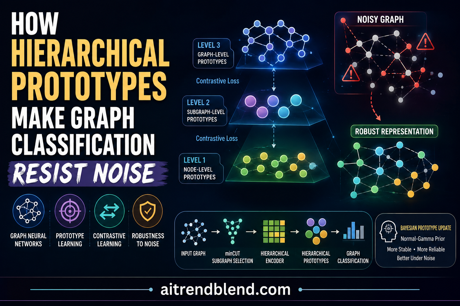
- HPGRL adds hierarchical contrastive regularization at the node, subgraph, and graph level, matching how a single corrupted edge or node cascades upward through a graph neural network.
- Subgraph and graph level embeddings are pulled toward continuous Gaussian prototypes estimated with an Expectation Maximization procedure rather than a fixed momentum average.
- A Bayesian Normal Gamma update refines class level prototypes batch by batch, which the authors argue produces tighter and more stable class clusters than a static class center.
- Across PROTEINS, COLLAB, IMDB-BINARY, IMDB-MULTI, Mutagenicity, and NCI1, the method beats eight recent baselines on five of the six datasets.
- Ablation and perturbation experiments show the subgraph level component contributes the most to both raw accuracy and robustness under node and edge corruption.
- The paper is a preprint posted on SSRN and has not yet been through formal peer review, a detail worth keeping in mind when weighing the reported numbers.
Why graph classifiers break so easily
Graph neural networks look deceptively sturdy on paper. Stack a few convolution layers, pool the node embeddings, feed the result to a classifier, and you get strong numbers on clean benchmark data. The trouble starts once the input graph stops being clean. Real molecular graphs come from noisy measurement pipelines. Real social graphs have missing edges because two people who actually know each other never happened to connect on the platform being scraped. Adversaries who want to fool a spam detector or a fraud graph can also add or remove a small number of edges on purpose.
The authors of this paper frame the core issue as a cascading effect. A perturbation at the node level, say a single feature vector getting corrupted, does not stay contained to that node. Message passing spreads the corruption to every neighbor within a few hops, then pooling spreads it again into the subgraph and graph level representations used for the final classification. By the time the signal reaches the classifier, a tiny local change has become a much larger shift in the graph level embedding.
Most existing fixes attack one layer of this problem at a time. Adversarial training hardens the model against a specific attack pattern. Graph structure learning tries to clean up the topology before the encoder ever sees it. Data augmentation generates synthetic variants so the model sees more diversity during training. Contrastive learning pulls together different views of the same graph so the encoder learns something more invariant. Each of these helps, but the paper argues none of them explicitly track the fact that noise can enter and compound at three different structural levels at once, and none of them separately model how stable the class boundaries themselves are once training data drifts.
What earlier prototype work got partly right
Prototype learning is not new to graph representation learning. Xu and colleagues used self supervised local and global structure objectives with learned prototypes. Lin and colleagues built a prototypical graph contrastive learning framework. Peng, Juan, and Li proposed graph prototypical contrastive learning aimed at unsupervised settings. What these approaches share is a focus on one level of representation, usually the graph as a whole, and a preference for discrete prototypes updated with a running average, sometimes called a momentum center.
The Dalian team points out a real weakness in that momentum approach. A single fixed average cannot represent the fact that a class in a graph dataset is rarely one tight cluster. It has spread, it has multiple modes, and a handful of outliers can drag the average off course. Continuous prototypes built from a Gaussian Mixture Model, estimated with the classic Expectation Maximization algorithm, handle this better because each data point gets a soft assignment across multiple Gaussian components rather than one hard vote. That soft assignment is the reason continuous prototypes are more resistant to a stray noisy sample throwing off the whole cluster center.
Takeaway
The central bet of this paper is that robustness needs to be enforced at every level a corruption can travel through, node, subgraph, and graph, and that the class prototypes used for the final decision need their own uncertainty aware treatment separate from the representation learning stage.
How HPGRL is put together
Strip away the notation and the architecture is a graph convolutional encoder wrapped in two regularizers that operate at different stages of the pipeline. The first regularizer, the Hierarchical Structure Prototype Guided Contrastive Learning Regularizer, works during representation learning and enforces consistency across the node, subgraph, and graph levels. The second, the Bayesian Class Prototype Guided Projector Regularizer, works after the graph level embedding has been projected into a lower dimensional space and models class level distribution stability.
Step one, perturb the encoder on purpose
Node features and the edge index of an input graph pass through a standard graph convolutional network to produce a base embedding. That embedding is then run through K independent dropout layers, each producing a slightly different perturbed version of the same node embedding. All the perturbed copies that came from the same original graph share the same label. This is a familiar trick from contrastive learning, generating multiple views of the same input so the model can be pushed to treat them as similar while treating views from different graphs as dissimilar.
Step two, node level contrastive loss
Within a single graph, one perturbed node embedding is picked as the anchor. The other K minus one perturbed copies of that same original node become positive pairs. Every other perturbed node, whether from the same graph or a different one in the batch, becomes a negative pair. The loss is a standard InfoNCE style contrastive objective built from cosine similarity and a temperature parameter.
Step three, cut the graph into subgraphs
Before subgraph level embeddings can exist, the graph needs to be partitioned. HPGRL borrows the minCut pooling idea, which was originally built for spectral clustering with graph neural networks. A learned assignment matrix scores how strongly each node belongs to each of a fixed number of clusters, produced by a small multilayer perceptron followed by softmax. The clustering is guided by a loss that rewards keeping strongly connected nodes in the same cluster and penalizes clusters of very uneven size.
Once the assignment matrix is available, the subgraph embeddings are simply the node embeddings pooled through that matrix. The paper’s hyperparameter sweep found that a subgraph count between four and eight worked best on the IMDB-BINARY dataset. Push the subgraph count past ten and accuracy drops sharply, because with an average of only about twenty nodes per IMDB graph, too many clusters means each subgraph shrinks down to almost a single node, which defeats the purpose of having a subgraph level at all.
Step four, subgraph level contrastive and prototype losses
The subgraph level combines two objectives. A subgraph to subgraph contrastive loss follows the same anchor and positive and negative structure as the node level loss, just applied to pooled subgraph embeddings. A separate subgraph to prototype loss assumes the subgraph embeddings for a given class follow an isotropic Gaussian distribution, with several prototype centers per class rather than one.
Instead of picking those centers by hand, the model estimates them with Expectation Maximization, run in two alternating steps on every batch. The E step uses K means clustering on the current batch of subgraph embeddings to estimate the prototype centers and to assign each embedding to its nearest prototype. The M step then plugs those centers and assignments into a softmax style loss over the Gaussian density, which pulls each subgraph embedding toward its assigned prototype and away from the others.
Running the clustering multiple times with different numbers of prototypes, then averaging the resulting loss, is a small but sensible robustness trick. It means the final loss does not depend too heavily on one particular guess about how many modes exist inside a class.
Step five, graph level loss and pooling to a single vector
Subgraph embeddings are pooled once more to produce a single graph level embedding. The same anchor, positive, negative contrastive setup runs at this level too, comparing full graph embeddings across the batch, alongside a graph to prototype loss built the same way as the subgraph version.
In the reported hyperparameters, the node level term gets a weight of just 0.001 while the graph level term gets a weight of 1, which tells you where the authors believe most of the useful signal sits. The subgraph term sits in between at 0.1. That weighting lines up with the ablation results discussed further down, where removing the subgraph component causes the single largest accuracy drop of any ablation.
The Bayesian class prototype layer
Everything up to this point is representation learning. The classification decision itself comes from a second module. The graph level embedding first passes through a one layer projection into a smaller dimensional space. Then, instead of learning one fixed vector per class the way a typical softmax classifier does, HPGRL treats each class as its own normal distribution with an unknown mean and variance, and updates the parameters of that distribution using Bayesian estimation rather than gradient descent alone.
Specifically, the mean and variance for each class follow a Normal Gamma distribution, the standard conjugate prior for a normal distribution with unknown mean and variance. Each new batch of graph embeddings that share a gold label gets folded into the running estimate through four update equations that adjust the posterior mean, the confidence in that mean, and the shape and scale of the variance estimate.
Maximum a posteriori estimation then turns those updated Normal Gamma parameters into a point estimate for the mean and variance of each class, which is what actually gets used at prediction time. Two extra loss terms shape how well separated the classes end up. An intra prototype term penalizes high variance within a class, effectively asking the model to keep each class tight. An inter prototype term rewards distance between the means of different classes.
This is essentially a Fisher discriminant idea wearing Bayesian clothing. Minimize spread inside a class, maximize spread between classes. What the Bayesian machinery adds on top is a principled way to update those class statistics batch by batch without simply overwriting the old estimate, since the Normal Gamma update naturally weighs new evidence against how confident the model already was.
Prediction itself falls out of the class conditional Gaussian densities. Given a new graph embedding, the model computes the probability under each class distribution using the MAP estimated mean and variance, applies a softmax across classes, and takes the highest scoring class as the prediction. Training then minimizes a standard cross entropy loss on top of that, alongside the clustering loss and the instance level prototype loss from the earlier stage.
Do the numbers hold up
The authors evaluate on six standard TUDataset benchmarks. IMDB-BINARY and IMDB-MULTI are actor co appearance graphs used for genre classification. COLLAB captures scientific collaboration networks labeled by research field. PROTEINS labels protein structures as enzyme or not. Mutagenicity and NCI1 are molecular graphs labeled for mutagenic or anti cancer properties respectively.
| Method | PROTEINS | COLLAB | IMDB-BINARY | IMDB-MULTI | Mutagenicity | NCI1 |
|---|---|---|---|---|---|---|
| CSSL 2021 | 60.71 | 80.48 | 72.40 | 52.79 | 76.85 | 71.56 |
| DualGraph 2022 | 62.32 | 67.20 | 72.10 | 44.80 | not reported | not reported |
| VIB-GSL 2022 | 61.60 | 78.30 | 74.10 | 54.30 | 69.63 | 65.10 |
| MGRL 2023 | 62.85 | 81.96 | 73.79 | 55.20 | 77.56 | 68.32 |
| OMG 2023 | 63.21 | not reported | 67.40 | 45.10 | 77.70 | 65.10 |
| AVCN 2024 | 64.82 | 80.24 | 74.02 | 51.35 | not reported | not reported |
| G-Prompt 2024 | not reported | 68.34 | 68.03 | 45.17 | not reported | 69.87 |
| G-MIMO 2024 | 65.31 | not reported | 76.00 | 51.13 | not reported | not reported |
| HPGRL, this paper | 64.73 | 82.57 | 76.23 | 59.37 | 79.47 | 71.67 |
All figures are accuracy percentages, averaged over five runs with different random seeds, and the plus or minus ranges from the paper are omitted here for readability but are worth checking in the original table before citing a specific figure. HPGRL comes out ahead on five of the six datasets. The one exception is PROTEINS, where G-MIMO edges it out by a little over half a point. The largest single margin shows up on IMDB-MULTI, where HPGRL beats the next best result, G-MIMO at 51.13, by more than four points. The authors also highlight a solid gain on Mutagenicity, where HPGRL beats the runner up OMG by roughly 1.8 points.
Worth noting for anyone comparing across the table, several baselines have blank cells for datasets their original papers simply did not test on, which is why DualGraph and OMG and G-Prompt and G-MIMO all have gaps. That is a normal feature of building a comparison table from several separate papers rather than evidence of missing effort on HPGRL’s part.
The biggest single point drop in the entire ablation table comes from removing the subgraph level, which is a strong hint that the middle layer of the hierarchy is doing more work than either the node or the graph level alone.Reading of the HPGRL ablation results, Table 3 in the source paper
What the ablation study actually shows
The authors test five stripped down variants. One removes the entire subgraph level. One removes prototype guided learning at the subgraph and graph level while keeping the contrastive part. One removes the contrastive part while keeping the prototypes. One removes both prototypes and contrastive learning at those two levels together. The last removes only the class level Bayesian optimization.
| Variant | IMDB-BINARY | NCI1 | IMDB-MULTI | Mutagenicity |
|---|---|---|---|---|
| Full HPGRL | 76.23 | 71.67 | 59.37 | 79.47 |
| Without subgraph level | 73.31 | 67.80 | 56.88 | 77.36 |
| Without prototype guidance | 76.01 | 70.75 | 58.42 | 78.94 |
| Without contrastive terms | 75.77 | 71.65 | 59.15 | 78.93 |
| Without prototype and contrastive | 74.99 | 69.62 | 57.94 | 78.31 |
| Without class optimization | 75.89 | 68.50 | 58.62 | 78.59 |
Removing the entire subgraph level costs almost three points on IMDB-BINARY and close to four points on NCI1, by far the largest single drop anywhere in the table. That lines up neatly with the low node level weight of 0.001 chosen in the hyperparameters. It reads as the authors having discovered during tuning that the middle layer of the hierarchy carries most of the useful signal, and the raw node level term mostly adds noise if weighted too heavily.
Removing just the class level Bayesian optimization also hurts, particularly on NCI1 where accuracy falls by more than three points, more than the drop from removing either the prototype or contrastive terms individually at the subgraph and graph level. That suggests the Bayesian class layer is not simply icing on top of a good encoder, it is pulling real weight on datasets where the class boundaries are harder to separate in the first place.
Does it actually stay robust under attack
The robustness section is where this paper earns its title. The authors apply two kinds of synthetic corruption. Node perturbation randomly replaces a fraction of node feature vectors with a different random one hot vector. Edge perturbation randomly adds or removes a percentage of edges.
Comparing full HPGRL against the stripped variant with both prototype and contrastive terms removed, accuracy stays consistently higher for the full model as the corruption rate climbs, across both the PROTEINS and NCI1 datasets. The two datasets react differently to the two perturbation types though. PROTEINS is noticeably more sensitive to edge perturbation than node perturbation, while NCI1 shows the opposite pattern, reacting more strongly to node level noise than to added or removed edges. That is a useful reminder that robustness interventions are not one size fits all, the right defense partly depends on what kind of graph you are working with.
A second robustness experiment looks at confidence rather than raw accuracy, measuring how much the model’s predicted probability shifts between a clean graph and its perturbed version, visualized with violin plots on IMDB-BINARY. Removing the subgraph level or the instance level prototype and contrastive terms both widen the spread of that confidence shift substantially. Removing only the class level optimization produces a smaller spread increase but a clear rightward shift in the average change, meaning predictions become less confidently stable even when the final label does not flip.
What the PCA and t-SNE plots add
Beyond the numeric tables, the authors run a small qualitative experiment. They pick six graphs, apply two hundred random node perturbations to each, and plot the resulting embeddings with PCA next to the original clean embedding. The full HPGRL model produces tight, well separated clusters around each original graph. Removing the class level optimization introduces visible overlap between at least one pair of classes. Removing the subgraph level makes that overlap considerably worse, with noticeably more inter class confusion than either of the other two variants. A parallel t-SNE experiment on the COLLAB and IMDB-BINARY validation and test sets tells a similar story, with the stripped down variant showing a class boundary that runs directly through a cluster of same class points, while full HPGRL keeps a visible gap between classes.
Is any of this expensive to run
A fair question for anyone considering this for production is whether all these extra losses blow up training time. The paper’s complexity analysis is reassuring on this point. The Expectation Maximization step, which is the most computationally heavy piece, scales with the chosen hyperparameters for prototype counts and batch size, not with the size of the input graphs. In other words, adding more nodes or edges to your graphs does not make the EM step slower. The one piece that does scale with graph size is the minCut pooling operation itself, which the authors note runs in time roughly proportional to the number of edges plus the number of nodes times the number of subgraph clusters, a linear relationship that should stay manageable outside of extremely dense graphs.
The K way dropout perturbation used to generate multiple views per graph does multiply the amount of node level data processed by a factor of K, but because those K views are generated in parallel rather than requiring separate rounds of message passing, the authors describe the overhead as manageable and dependent on batch size rather than graph size.
Takeaway
The extra machinery in HPGRL is front loaded into hyperparameter heavy components, prototype counts, cluster counts, and perturbation counts, rather than into anything that grows with the size of individual graphs, which matters if you are thinking about applying this to larger graphs than the TUDataset benchmarks used here.
Honest limitations
This is a preprint hosted on SSRN and has not gone through formal peer review at the time this article was written, so the reported numbers have not yet been independently checked by reviewers outside the author group.
The benchmark graphs used here are small by real world standards, IMDB-MULTI graphs average only thirteen nodes and COLLAB graphs average around seventy four, so it remains an open question how the hierarchical scheme behaves on graphs with thousands of nodes where subgraph partitioning becomes a much harder problem.
Several baseline comparisons rely on numbers copied from each baseline’s original publication rather than being rerun by the HPGRL authors under identical conditions, which is common practice but means differences in hardware, hyperparameter search budget, and code implementation could contribute to some of the reported gaps.
The paper does not report wall clock training time or GPU memory usage for HPGRL against the baselines, only asymptotic complexity, so anyone evaluating this for a resource constrained setting will need to benchmark it themselves.
The hyperparameter search space, including the number of perturbations, subgraph counts, and temperature values, is fairly wide, and the paper does not report how sensitive final accuracy is to small deviations from the chosen values beyond the single subgraph count sweep shown for IMDB-BINARY.
Where this fits in the bigger picture
Step back from the equations and HPGRL is really an argument about where robustness work should be spent. A lot of recent graph robustness research has focused on either cleaning the input graph before it reaches the model or hardening the model against a specific attack pattern. This paper instead argues for treating robustness as a representation learning problem that needs attention at every scale a graph naturally decomposes into. That framing generalizes well beyond graph classification. Any hierarchical data structure, from parse trees in natural language processing to scene graphs in computer vision, faces a similar cascading effect where a small local error compounds as it moves up through the pooling stages of a model. Researchers working in those adjacent areas may find the general recipe of level specific contrastive losses paired with a Bayesian class layer worth borrowing even outside graph classification specifically.
Complete PyTorch implementation
The paper describes the architecture in full mathematical detail but does not release code alongside it. Below is an independent, runnable reimplementation of the core ideas, built with plain PyTorch and dense adjacency matrices so it has no dependency on a graph library. It includes the perturbed graph convolutional encoder, the three level contrastive regularizer, a simplified minCut style subgraph pooling step, EM style prototype estimation using K means, the Bayesian Normal Gamma class prototype update, the combined loss, a training loop, an evaluation function, and a smoke test on randomly generated dummy graphs.
# hpgrl_reimplementation.py
# Independent PyTorch reimplementation of the HPGRL architecture described in
# "Hierarchical Prototype Guided Representation Learning for Robust Graph
# Classification" by Zhang, Chen, Jin, and Wei. This is not the authors' own
# code, it is a reconstruction built from the equations in the paper for
# educational use.

import torch
import torch.nn as nn
import torch.nn.functional as F
import math

class GraphConvLayer(nn.Module):
    # A minimal dense graph convolution, X_out = A_hat @ X @ W
    def __init__(self, in_dim, out_dim):
        super().__init__()
        self.linear = nn.Linear(in_dim, out_dim)

    def forward(self, x, adj):
        # x has shape [batch, nodes, in_dim], adj has shape [batch, nodes, nodes]
        deg = adj.sum(dim=-1, keepdim=True).clamp(min=1.0)
        adj_norm = adj / deg
        agg = torch.bmm(adj_norm, x)
        return F.relu(self.linear(agg))


class PerturbedGraphEncoder(nn.Module):
    def __init__(self, in_dim, hidden_dim, dropout_rate=0.5):
        super().__init__()
        self.gcn1 = GraphConvLayer(in_dim, hidden_dim)
        self.gcn2 = GraphConvLayer(hidden_dim, hidden_dim)
        self.dropout_rate = dropout_rate

    def forward(self, x, adj):
        h = self.gcn1(x, adj)
        h = self.gcn2(h, adj)
        return h  # base node embeddings E

    def perturb(self, e, k):
        # produce k independently dropped out copies of the base embedding
        views = [F.dropout(e, p=self.dropout_rate, training=True) for _ in range(k)]
        return torch.stack(views, dim=0)  # [k, batch, nodes, hidden_dim]


def info_nce_loss(anchor, positives, negatives, temperature):
    # anchor [d], positives [p, d], negatives [n, d]
    pos_sim = F.cosine_similarity(anchor.unsqueeze(0), positives, dim=-1) / temperature
    neg_sim = F.cosine_similarity(anchor.unsqueeze(0), negatives, dim=-1) / temperature
    numerator = torch.exp(pos_sim).sum()
    denominator = numerator + torch.exp(neg_sim).sum()
    return -torch.log(numerator / denominator.clamp(min=1e-8))


class MinCutPooling(nn.Module):
    # Simplified minCut style soft clustering used to build subgraph embeddings
    def __init__(self, hidden_dim, num_clusters):
        super().__init__()
        self.assign = nn.Linear(hidden_dim, num_clusters)
        self.num_clusters = num_clusters

    def forward(self, node_emb, adj):
        # node_emb [batch, nodes, hidden_dim], adj [batch, nodes, nodes]
        s = F.softmax(self.assign(node_emb), dim=-1)  # [batch, nodes, clusters]
        sub_emb = torch.bmm(s.transpose(1, 2), node_emb)  # [batch, clusters, hidden_dim]

        num = torch.einsum('bnk,bnm,bmk->bk', s, adj, s)
        deg = adj.sum(dim=-1)
        den = torch.einsum('bnk,bn->bk', s, deg).clamp(min=1e-8)
        cut_loss = -(num / den).mean()

        st_s = torch.bmm(s.transpose(1, 2), s)
        st_s_norm = st_s / st_s.norm(dim=(1, 2), keepdim=True).clamp(min=1e-8)
        identity = torch.eye(self.num_clusters, device=s.device) / math.sqrt(self.num_clusters)
        ortho_loss = (st_s_norm - identity).norm(dim=(1, 2)).mean()

        return sub_emb, cut_loss, ortho_loss


def em_prototype_loss(embeddings, num_prototypes, temperature=0.2, kmeans_iters=5):
    # E step, plain K means on the current batch of embeddings
    with torch.no_grad():
        perm = torch.randperm(embeddings.size(0))[:num_prototypes]
        centers = embeddings[perm].clone()
        for _ in range(kmeans_iters):
            dists = torch.cdist(embeddings, centers)
            assign = dists.argmin(dim=1)
            for c in range(num_prototypes):
                mask = assign == c
                if mask.any():
                    centers[c] = embeddings[mask].mean(dim=0)

    # M step, pull each embedding toward its assigned prototype
    sims = torch.matmul(embeddings, centers.t()) / temperature
    log_probs = F.log_softmax(sims, dim=-1)
    loss = F.nll_loss(log_probs, assign)
    return loss, centers


class BayesianClassPrototype(nn.Module):
    # Maintains a Normal Gamma posterior per class and produces MAP mean and variance
    def __init__(self, num_classes, proj_dim, prior_mu=0.0, prior_lambda=1.0, prior_alpha=1.0, prior_beta=1.0):
        super().__init__()
        self.num_classes = num_classes
        self.proj_dim = proj_dim
        self.register_buffer('mu', torch.full((num_classes, proj_dim), prior_mu))
        self.register_buffer('lam', torch.full((num_classes,), prior_lambda))
        self.register_buffer('alpha', torch.full((num_classes,), prior_alpha))
        self.register_buffer('beta', torch.full((num_classes,), prior_beta))

    def update(self, embeddings, labels):
        for c in range(self.num_classes):
            mask = labels == c
            s_n = mask.sum().item()
            if s_n == 0:
                continue
            batch = embeddings[mask]
            x_bar = batch.mean(dim=0)
            gamma2 = batch.var(dim=0, unbiased=False).mean()

            lam_old, mu_old, alpha_old, beta_old = self.lam[c].clone(), self.mu[c].clone(), self.alpha[c].clone(), self.beta[c].clone()
            self.mu[c] = (lam_old * mu_old + s_n * x_bar) / (lam_old + s_n)
            self.lam[c] = lam_old + s_n
            self.alpha[c] = alpha_old + s_n / 2.0
            self.beta[c] = beta_old + 0.5 * (s_n * gamma2 + (s_n * lam_old * (x_bar - mu_old).pow(2).mean()) / (lam_old + s_n))

    def map_estimate(self):
        mu_map = self.mu
        var_map = (self.alpha - 0.5) / self.beta.clamp(min=1e-8)
        return mu_map, var_map.clamp(min=1e-6)

    def class_separation_loss(self):
        mu_map, var_map = self.map_estimate()
        l_intra = var_map.sum()
        diffs = mu_map.unsqueeze(0) - mu_map.unsqueeze(1)
        l_inter = diffs.pow(2).sum()
        return -torch.log((l_inter.clamp(min=1e-8)) / l_intra.clamp(min=1e-8))

    def predict(self, embeddings):
        mu_map, var_map = self.map_estimate()
        # log density of an isotropic Gaussian per class, summed over dimensions
        diffs = embeddings.unsqueeze(1) - mu_map.unsqueeze(0)
        log_prob = -0.5 * (diffs.pow(2) / var_map.unsqueeze(0).unsqueeze(0)).sum(dim=-1)
        log_prob = log_prob - 0.5 * self.proj_dim * torch.log(2 * math.pi * var_map).sum(dim=0) / self.num_classes
        return F.softmax(log_prob, dim=-1)


class HPGRL(nn.Module):
    def __init__(self, in_dim, hidden_dim, proj_dim, num_classes, num_subgraphs=6, k_views=4):
        super().__init__()
        self.encoder = PerturbedGraphEncoder(in_dim, hidden_dim)
        self.pooling = MinCutPooling(hidden_dim, num_subgraphs)
        self.graph_readout = nn.Linear(hidden_dim, hidden_dim)
        self.projector = nn.Linear(hidden_dim, proj_dim)
        self.bayes = BayesianClassPrototype(num_classes, proj_dim)
        self.k_views = k_views

    def forward(self, x, adj, labels, node_temp=0.5, sub_temp=0.5, graph_temp=0.5):
        base_emb = self.encoder(x, adj)  # [batch, nodes, hidden]
        views = self.encoder.perturb(base_emb, self.k_views)  # [k, batch, nodes, hidden]
        k, batch, nodes, hidden = views.shape

        node_losses = []
        sub_losses = []
        graph_losses = []
        graph_embs_per_view = []
        cut_losses = []
        ortho_losses = []

        for b in range(batch):
            flat_nodes = views[:, b].reshape(k * nodes, hidden)
            anchor_idx = 0
            anchor = flat_nodes[anchor_idx]
            pos_idx = [i * nodes for i in range(1, k)]
            positives = flat_nodes[pos_idx] if len(pos_idx) > 0 else flat_nodes[1:2]
            neg_mask = torch.ones(flat_nodes.size(0), dtype=torch.bool)
            neg_mask[[anchor_idx] + pos_idx] = False
            negatives = flat_nodes[neg_mask]
            if negatives.size(0) > 0:
                node_losses.append(info_nce_loss(anchor, positives, negatives, node_temp))

        sub_embs_per_view = []
        for v in range(k):
            sub_emb, cut_l, ortho_l = self.pooling(views[v], adj)
            sub_embs_per_view.append(sub_emb)
            cut_losses.append(cut_l)
            ortho_losses.append(ortho_l)
        sub_embs_per_view = torch.stack(sub_embs_per_view, dim=0)  # [k, batch, clusters, hidden]

        for b in range(batch):
            flat_subs = sub_embs_per_view[:, b].reshape(k * sub_embs_per_view.size(2), hidden)
            anchor = flat_subs[0]
            positives = flat_subs[1:min(k, flat_subs.size(0))]
            negatives = flat_subs[min(k, flat_subs.size(0)):]
            if positives.size(0) > 0 and negatives.size(0) > 0:
                sub_losses.append(info_nce_loss(anchor, positives, negatives, sub_temp))

        graph_embs = self.graph_readout(sub_embs_per_view.mean(dim=2))  # [k, batch, hidden]
        for b in range(batch):
            anchor = graph_embs[0, b]
            positives = graph_embs[1:, b]
            other_mask = torch.ones(batch, dtype=torch.bool)
            other_mask[b] = False
            negatives = graph_embs[0][other_mask]
            if positives.size(0) > 0 and negatives.size(0) > 0:
                graph_losses.append(info_nce_loss(anchor, positives, negatives, graph_temp))

        graph_flat = graph_embs.mean(dim=0)  # [batch, hidden], averaged across the k perturbed views
        sub_proto_loss, _ = em_prototype_loss(sub_embs_per_view.mean(dim=0).reshape(-1, hidden), num_prototypes=min(3, batch))
        graph_proto_loss, _ = em_prototype_loss(graph_flat, num_prototypes=min(3, batch))

        proj = self.projector(graph_flat)
        self.bayes.update(proj.detach(), labels)
        class_loss = self.bayes.class_separation_loss()
        probs = self.bayes.predict(proj)
        ce_loss = F.nll_loss(torch.log(probs.clamp(min=1e-8)), labels)

        l_node = torch.stack(node_losses).mean() if node_losses else torch.tensor(0.0)
        l_sub_contrast = torch.stack(sub_losses).mean() if sub_losses else torch.tensor(0.0)
        l_graph_contrast = torch.stack(graph_losses).mean() if graph_losses else torch.tensor(0.0)
        l_cluster = (torch.stack(cut_losses).mean() + torch.stack(ortho_losses).mean())

        l_subgraph = 0.1 * l_sub_contrast + 1.0 * sub_proto_loss
        l_graph = 1.0 * l_graph_contrast + 1.0 * graph_proto_loss
        l_instance = 0.001 * l_node + 0.1 * l_subgraph + 1.0 * l_graph

        total_loss = l_instance + class_loss + l_cluster + ce_loss
        return total_loss, probs


def train_step(model, optimizer, x, adj, labels):
    model.train()
    optimizer.zero_grad()
    loss, probs = model(x, adj, labels)
    loss.backward()
    optimizer.step()
    return loss.item()


def evaluate(model, x, adj, labels):
    model.eval()
    with torch.no_grad():
        _, probs = model(x, adj, labels)
        preds = probs.argmax(dim=-1)
        acc = (preds == labels).float().mean().item()
    return acc


if __name__ == '__main__':
    # Smoke test on randomly generated dummy graphs, no real dataset needed
    torch.manual_seed(0)
    batch_size, num_nodes, in_dim, hidden_dim, proj_dim, num_classes = 8, 15, 10, 32, 16, 3

    x = torch.randn(batch_size, num_nodes, in_dim)
    adj = (torch.rand(batch_size, num_nodes, num_nodes) > 0.7).float()
    adj = adj + adj.transpose(1, 2)
    adj = (adj > 0).float()
    labels = torch.randint(0, num_classes, (batch_size,))

    model = HPGRL(in_dim, hidden_dim, proj_dim, num_classes, num_subgraphs=4, k_views=3)
    optimizer = torch.optim.Adam(model.parameters(), lr=1e-3)

    for epoch in range(5):
        loss_val = train_step(model, optimizer, x, adj, labels)
        acc = evaluate(model, x, adj, labels)
        print(f'epoch {epoch} loss {loss_val:.4f} train batch accuracy {acc:.4f}')

    print('Smoke test complete, model trains end to end on dummy data without errors.')
Conclusion
The core achievement here is fairly narrow on paper but broad in effect. HPGRL takes an idea that has floated around graph representation learning for a while, that prototypes make representations more stable, and pushes it through every level a graph naturally decomposes into rather than applying it once at the top. That single design choice, backed up by the ablation table showing the subgraph level carries the most weight, is the paper’s real contribution.
The conceptual shift worth sitting with is the move away from treating class centers as fixed points learned once and reused. Modeling each class as a full Normal Gamma posterior that updates batch by batch is a small piece of Bayesian machinery, but it reframes classification as an ongoing estimation problem rather than a one time fit, which fits naturally with how real world graph data tends to arrive in a continuous stream rather than a single static file.
Transferability beyond graph classification looks genuinely promising. Any domain where a small unit level signal gets pooled up through intermediate structures before a final decision, document classification built from sentence and paragraph embeddings, video understanding built from frame and clip embeddings, or even multi agent systems where individual agent states get pooled into a team level representation, could plausibly borrow the same hierarchical prototype recipe.
The honest limitations should not be glossed over. This is preprint work on relatively small benchmark graphs, several baseline numbers are borrowed rather than reproduced under identical conditions, and there is no reported wall clock cost comparison against the baselines. None of that erases the value of the ablation and robustness experiments, which are unusually thorough for a paper of this length, but it does mean the headline accuracy numbers deserve a healthy dose of patience until independent replication and formal peer review catch up.
Where this goes next probably depends on whether someone scales the same hierarchical prototype idea up to graphs with thousands or millions of nodes, where subgraph partitioning becomes a genuinely hard combinatorial problem rather than a clean minCut operation on a twenty node social graph. Until that test happens, the safest read is that HPGRL offers a well reasoned and carefully ablated argument for multi level prototype guidance, one that a graph learning practitioner should absolutely try on their own noisy dataset before assuming it generalizes past the six benchmarks tested here.
Frequently asked questions
What does HPGRL actually stand for and what problem does it solve
HPGRL stands for Hierarchical Prototype Guided Representation Learning. It targets the problem of graph neural networks losing accuracy when the input graph contains noise, missing edges, or small adversarial changes, by enforcing consistency at the node, subgraph, and graph level simultaneously rather than at just one level.
How is this different from ordinary graph contrastive learning
Ordinary graph contrastive learning usually compares two full graph views against each other. HPGRL adds two more comparison levels underneath that, node level and subgraph level, and adds continuous Gaussian prototypes estimated with Expectation Maximization at the subgraph and graph level rather than relying purely on instance to instance contrast.
What is the Bayesian class prototype actually doing
It treats each class as an unknown normal distribution and updates the estimate of that distribution’s mean and variance batch by batch using a Normal Gamma conjugate prior, then uses a maximum a posteriori estimate of that distribution for classification, instead of learning one fixed vector per class the way a typical softmax layer does.
Which datasets was HPGRL tested on
Six TUDataset benchmarks, PROTEINS, COLLAB, IMDB-BINARY, IMDB-MULTI, Mutagenicity, and NCI1, covering protein structure classification, collaboration network field prediction, movie genre prediction from actor graphs, and molecular property prediction.
Does the paper prove HPGRL is robust to real adversarial attacks
It tests robustness against random node feature corruption and random edge addition or removal, not against an adaptive adversary specifically optimizing an attack against the model, so the robustness claims are best read as resilience to random noise rather than a guarantee against a determined attacker.
Has this paper been peer reviewed
No, it is currently posted as a preprint on SSRN and states directly that it has not been peer reviewed, so the reported results have not yet been independently verified through the normal journal or conference review process.
Read the full paper for the complete derivations, additional ablation figures, and the authors’ hyperparameter search details.