
Key points
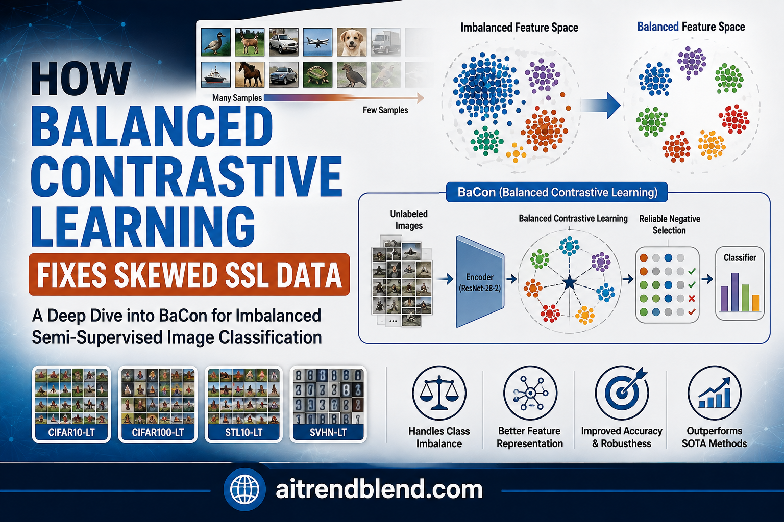
- BaCon adds a feature level contrastive loss on top of existing semi supervised learning pipelines to directly balance the distribution of learned representations.
- Class feature centers computed from a memory bank act as positive anchors, while a Reliable Negative Selection scheme picks trustworthy negative samples from both labeled and unlabeled data.
- A Balanced Temperature Adjusting mechanism gives tail classes a gentler pull toward their feature center early in training, since that center is less reliable when it is built from only a few samples.
- Across CIFAR10-LT, CIFAR100-LT, STL10-LT, and SVHN-LT, BaCon beats the current best instance level method ABC and the current best feature level method CoSSL in almost every tested setting.
- BaCon shows its biggest advantage when labeled and unlabeled data have opposite imbalance directions, a stress test where a rival method called CoSSL loses nearly twelve points of accuracy while BaCon barely moves.
- A short exploration experiment in the paper, training the same auxiliary classifier on a frozen balanced representation versus a frozen imbalanced one, is really the whole argument for the method in miniature.
Why imbalance breaks semi supervised learning twice over
Semi supervised learning exists to squeeze more value out of unlabeled data when labeling everything by hand is too expensive. Methods such as FixMatch and ReMixMatch have gotten very good at this under one quiet assumption, that every class shows up roughly the same number of times in both the labeled set and the pile of unlabeled data sitting alongside it. Real datasets rarely cooperate. Medical scans of rare conditions, security footage of unusual events, and product photos of niche items all show up far less often than the common cases, and that skew shows up in the unlabeled pool just as much as the labeled one.
The paper frames this as Class Imbalanced Semi Supervised Learning, shortened to CISSL, and points out a compounding problem specific to the semi supervised setting. A model trained on skewed data tends to produce pseudo labels that lean toward the majority class, and those biased pseudo labels then get fed right back into training as if they were ground truth. The imbalance in the original data and the imbalance introduced by unreliable pseudo labeling reinforce each other, which is a nastier problem than plain class imbalance in a fully supervised setting.
What earlier fixes got right and where they stopped short
Most existing CISSL methods work at what the paper calls the instance level, adjusting which samples get more weight or get resampled during training. DARP softly refines pseudo labels by solving an optimization problem. A reverse sampling approach from Wei and colleagues noticed that models tend to have decent precision but poor recall on minority classes and resamples accordingly. ABC, short for Auxiliary Balanced Classifier, attaches a second classification head next to the main one and applies a Bernoulli mask that is set inversely proportional to how common each predicted class is, giving rarer classes more influence during that head’s training.
A separate method called CoSSL takes a different route, decoupling representation learning from classifier learning and increasing the diversity of minority class data through feature blending. The BaCon authors point out a real weakness here too, feature blending can introduce noise and it quietly assumes the labeled data and unlabeled data follow a similar distribution, an assumption that will not always hold in practice.
What all of these instance level approaches share, according to the paper, is that they leave the upstream feature extractor mostly untouched. Reweighting which samples the classifier pays attention to does nothing to fix the representations those samples get turned into in the first place. If the feature space itself is skewed toward the majority class, no amount of classifier level rebalancing can fully undo that.
Takeaway
The central claim of this paper is that class imbalance in semi supervised learning is at least partly a representation problem, not just a classifier problem, and that fixing the feature space directly should pay off more than reweighting predictions after the fact.
The experiment that motivates the whole method
Before proposing anything new, the authors run a small but telling experiment on CIFAR10-LT. They train ABC two different ways. In the normal setup, the backbone feature extractor and the auxiliary classifier train together for three hundred thousand iterations, the standard procedure. In the comparison setup, the backbone is first trained by itself on a class balanced version of the same total number of samples for three hundred thousand iterations, producing a feature extractor that never saw imbalance. That backbone is then frozen, and only the auxiliary classifier trains on the actual imbalanced CIFAR10-LT data for another three hundred thousand iterations.
The normally trained version reaches 82.48 percent accuracy. The version built on a frozen balanced representation reaches 88.60 percent, a jump of more than six points from changing nothing except how balanced the upstream features were. That gap is the entire justification for BaCon. A perfectly balanced representation is not something you can produce directly in a real imbalanced dataset, since you would need balanced data to train it in the first place, but the experiment shows how much is on the table if you can nudge the representation in that direction even approximately.
The base pipeline BaCon plugs into
BaCon is designed as an add on component rather than a replacement for existing semi supervised learning pipelines. The paper builds on top of ABC layered over FixMatch, so it is worth walking through that base pipeline first. For a K class problem with labeled data X and unlabeled data U, FixMatch computes a standard supervised loss on labeled examples and an unsupervised consistency loss on unlabeled examples, using the model’s own confident predictions on a weakly augmented image as a pseudo label for training against a strongly augmented version of that same image.
ABC adds an auxiliary classification head that performs the same two kinds of learning, but applies a Bernoulli mask set inversely proportional to how large a predicted class currently appears to be, so the auxiliary head effectively downsamples the majority classes on the fly.
The same masked training happens on the unlabeled consistency loss, and the full backbone objective sums all four pieces together.
This is exactly the setup whose limitation the motivating experiment exposed. Both the original backbone head and the auxiliary head send gradients back into the shared feature extractor, and those two gradient signals pull in different directions, one biased by the raw imbalanced data and one artificially rebalanced by the Bernoulli mask. The net effect on the representation layer ends up somewhere between the two, and nowhere close to the ideal balanced direction that the frozen backbone experiment showed was achievable.
How BaCon regularizes the feature space directly
BaCon adds a third loss term aimed squarely at the representation layer, sitting alongside the backbone and auxiliary classifier losses rather than replacing them. A small linear projection head maps the backbone representation into a separate contrastive space where the new loss operates.
Building reliable class feature centers
To get positive learning targets, BaCon keeps a running memory bank of instance features, but only accepts a feature into that memory bank if the auxiliary classifier’s confidence for that prediction clears a high threshold, set to 0.98 by default. This filtering step matters because pseudo labels on unlabeled data are not always trustworthy, and letting a wrong label pollute the memory bank would corrupt every class center built from it. A second memory bank tracks which class each stored feature belongs to, using the true label for labeled data and the auxiliary head’s prediction for unlabeled data. The feature center for each class is then just the average of everything currently stored for that class, and that average becomes the positive anchor point for every sample of that class during contrastive training.
The full BaCon contrastive loss then pulls each instance toward its own class anchor while pushing it away from a set of negative samples, following a shape similar to the well known InfoNCE objective from self supervised learning.
Choosing negatives without drowning in noise or starving for data
Picking good negative samples turned out to be its own design problem. Using only labeled data as negatives keeps the signal clean but shrinks the negative pool badly, since labeled data is scarce by definition in this setting. Treating every sample not currently predicted as class k as a negative solves the size problem but drags in a lot of unreliable pseudo labeled noise. The Reliable Negative Selection scheme, shortened to RNS, threads that needle. For labeled data, any sample above the confidence threshold and belonging to a different class becomes a reliable negative. For unlabeled data, RNS ranks each sample’s predicted confidence across all classes and only treats a sample as a reliable negative for class k if class k does not appear within that sample’s top few most confident predictions, with the cutoff set to three by default. A sample that is not confidently class k, but also is not clearly excluded from it, gets left out of the negative pool entirely rather than risking a wrong signal.
Because the pool of reliable negatives for a given class can shrink or grow a lot from batch to batch, the weight applied to the negative term is scaled by the batch size relative to how many reliable negatives are currently available, which keeps the loss from swinging wildly when the negative count happens to be small in a particular mini batch.
Giving tail classes a gentler pull with Balanced Temperature Adjusting
Simple attraction toward a class center already helps, but the authors noticed a subtlety. A feature center for a class with very few samples is a shakier estimate of where that class truly sits, so pulling instances toward it too aggressively risks reinforcing an already noisy target. The Balanced Temperature Adjusting mechanism, shortened to BTA, addresses this by scaling the temperature of the positive pull per class according to how large that class currently appears to be relative to the largest class, with the gap between classes narrowing as training progresses and the class centers become more trustworthy.
Training itself happens in two stages. The backbone semi supervised algorithm and the auxiliary classifier train alone first, long enough to warm up the memory banks with reasonably trustworthy features, and only after that warmup period ends does the BaCon contrastive loss get added into the total objective.
At prediction time, only the auxiliary classifier’s output gets used to pick the final class, the projection head and the memory banks exist purely to shape training and play no role once training is finished.
Does it actually beat the current best methods
The authors test on four imbalanced benchmarks built from CIFAR10, CIFAR100, STL10, and SVHN, following a long tail construction where class size decreases exponentially according to a chosen imbalance ratio. CIFAR10-LT and SVHN-LT use an imbalance ratio of 100 with 20 percent of data labeled, CIFAR100-LT uses a ratio of 20 with 40 percent labeled, and STL10-LT uses a labeled ratio of 10, with the network built on a Wide ResNet-28-2 backbone throughout.
| Backbone and method | CIFAR10-LT | CIFAR100-LT | STL10-LT | SVHN-LT |
|---|---|---|---|---|
| FixMatch alone | 75.30 | 53.94 | 67.16 | 92.63 |
| FixMatch with DASO | 74.78 | 54.83 | 68.69 | 90.24 |
| FixMatch with CReST+PDA | 78.64 | 55.01 | 67.17 | 93.23 |
| FixMatch with SAW | 80.12 | 55.87 | 70.51 | 92.92 |
| FixMatch with ABC | 83.25 | 56.91 | 71.23 | 94.15 |
| FixMatch with CoSSL | 84.09 | 57.33 | 70.95 | 93.39 |
| FixMatch with BaCon | 84.46 | 57.96 | 71.55 | 94.54 |
| ReMixMatch with ABC | 84.49 | 59.92 | 67.24 | 94.03 |
| ReMixMatch with CoSSL | 84.93 | 60.46 | 68.73 | 92.26 |
| ReMixMatch with BaCon | 85.05 | 60.15 | 69.26 | 94.35 |
All numbers are balanced accuracy percentages measured on a class balanced test set. Built on FixMatch, BaCon beats CoSSL by 0.37 points on CIFAR10-LT, by 0.63 points on CIFAR100-LT, and by 0.60 points on STL10-LT, while also edging out ABC on every one of the four datasets. Built on ReMixMatch, BaCon beats CoSSL on CIFAR10-LT and SVHN-LT but falls slightly behind CoSSL on CIFAR100-LT by roughly three tenths of a point and on STL10-LT by about half a point. Those two exceptions are worth flagging honestly rather than glossing over, since the paper’s abstract highlights the wins without dwelling on where CoSSL still edges ahead under the ReMixMatch backbone.
A method that only wins when the labeled and unlabeled data happen to agree on which classes are rare is not solving the general problem, it is solving an easier special case of it.Reading of the BaCon stress test results, Table 2 in the source paper
What happens when the imbalance gets nastier
The most interesting result in the paper shows up in a stress test most methods are not built to survive. Beyond the standard setting where labeled and unlabeled data share the same imbalance direction, the authors also test a scenario where the two are inversely proportional, meaning the class that is rare among labeled examples is actually common among unlabeled ones and vice versa.
| Method | Matched ratio 100 | Inverse ratio 100 | Matched ratio 150 | Inverse ratio 150 |
|---|---|---|---|---|
| FixMatch alone | 75.66 | 56.35 | 73.45 | 62.30 |
| FixMatch with CReST+PDA | 79.14 | 66.47 | 74.51 | 62.75 |
| FixMatch with ABC | 82.48 | 81.14 | 79.41 | 78.84 |
| FixMatch with CoSSL | 83.94 | 71.99 | 81.83 | 74.14 |
| FixMatch with BaCon | 84.61 | 83.80 | 81.99 | 82.35 |
CoSSL drops from 83.94 percent in the matched setting all the way down to 71.99 percent once the imbalance direction flips, a fall of close to twelve points. That kind of collapse points to CoSSL leaning on an assumption that labeled and unlabeled data share a similar distribution, an assumption the feature blending step in CoSSL depends on more than its authors may have anticipated. ABC holds up noticeably better, dropping only about a point in the same comparison. BaCon barely moves at all, staying within roughly one point of its matched setting score across every one of the four tested configurations, and beating the second best method by 2.66 points in the ratio 100 inverse case and by 3.51 points in the ratio 150 inverse case.
What the ablation numbers reveal about which piece matters most
The authors strip BaCon down piece by piece on CIFAR10-LT built on FixMatch. A baseline auxiliary classifier alone reaches 83.95 percent. Adding the contrastive loss with Reliable Negative Selection pushes that to 84.30 percent. Interestingly, adding a naive version of Balanced Temperature Adjusting without any iteration based decay actually hurts, dropping accuracy to 83.87 percent once RNS is removed from that comparison, which suggests a badly tuned temperature schedule can undo the benefit of the contrastive loss entirely. Only once the decay term is added back does the full combination reach the best reported result of 84.61 percent.
| Contrastive loss | RNS | Naive BTA | Decayed BTA | Accuracy |
|---|---|---|---|---|
| yes | yes | no | no | 84.30 |
| yes | no | yes | no | 83.87 |
| yes | yes | yes | no | 84.15 |
| yes | yes | no | yes | 84.61 |
A separate sweep tests how the projection head’s output dimension affects results. Skipping the projection entirely, using the raw backbone representation directly in the contrastive loss, produces the worst result at 82.86 percent. A thirty two dimensional linear projection performs best at 84.61 percent, while a nonlinear projection built by adding a ReLU layer actually underperforms the plain linear version at 83.95 percent. The authors reason that a nonlinear layer can filter out information that is directly useful for classification, something that matters more in this setting than in the pure self supervised pretraining tasks where nonlinear projection heads are more common.
| Projection type | Identity | Nonlinear | 32 dim linear | 128 dim linear | 512 dim linear |
|---|---|---|---|---|---|
| Accuracy | 82.86 | 83.95 | 84.61 | 83.48 | 82.64 |
What the t-SNE plots actually show
Numbers aside, the paper includes a qualitative check that is easy to appreciate at a glance. The authors visualize the balanced CIFAR10 test set representations with t-SNE for three versions, plain FixMatch, FixMatch with ABC, and FixMatch with BaCon. Plain FixMatch produces representations with no clear separation between classes at all. Adding ABC introduces some structure, distinguishable clusters start to appear, but a lot of points from different classes still overlap in confusing ways. BaCon produces the cleanest separation of the three, with class clusters that are visibly more distinct from each other, which lines up with the paper’s central claim that regularizing the feature space directly produces a more useful representation than adjusting the classifier alone.
Honest limitations
The paper reports every main experiment on Wide ResNet-28-2 with a single RTX 3090 GPU, so it remains untested whether the same gains hold on larger backbones or at the resolution and scale of datasets well beyond CIFAR and STL10.
BaCon relies on a confidence threshold of 0.98 to decide which features enter the memory bank, and a top three ranking cutoff for reliable negative selection, both fixed defaults that the paper does not stress test extensively across other values, so their sensitivity outside the tested range is not fully known.
The warmup schedule fixes the first one hundred thousand of three hundred thousand total iterations before the contrastive loss activates, and the paper does not report how sensitive final accuracy is to shortening or lengthening that warmup window.
On the ReMixMatch backbone, BaCon does not consistently beat CoSSL, falling slightly behind on CIFAR100-LT and STL10-LT, a detail that deserves equal weight alongside the wins reported elsewhere in the same table.
The Balanced Temperature Adjusting formula depends on knowing the total number of training iterations T in advance to compute its decay term, which means it is tuned for a fixed length training run rather than an open ended or continually updated training setting.
Where this fits in the wider computer vision picture
Zoom out and BaCon is really making an argument that applies well beyond semi supervised image classification specifically. Any pipeline that trains a classifier on top of a shared feature extractor, and that faces a skewed distribution of classes, faces some version of the same conflicting gradient problem the motivating ABC experiment exposed. Object detectors trained on long tailed real world categories, video action recognition models where common actions vastly outnumber rare ones, and even multi label tagging systems for user generated content all share this same structural issue of a biased upstream representation limiting how much a downstream rebalancing trick can achieve. The general recipe here, using class feature centers as contrastive anchors and adjusting the pull strength based on how reliable each class estimate currently is, looks like a reasonable pattern to borrow in any of those adjacent computer vision settings, not just the semi supervised benchmarks tested in this specific paper.
Complete PyTorch implementation
The paper describes every loss term precisely but does not release its own code. Below is an independent reimplementation covering the projection head, the dual memory banks with confidence filtering, class feature center computation, Reliable Negative Selection, Balanced Temperature Adjusting, the full BaCon loss, a simplified FixMatch plus ABC backbone, a training loop, an evaluation function, and a smoke test on randomly generated dummy data so it runs without needing an actual imbalanced image dataset.
# bacon_reimplementation.py
# Independent PyTorch reimplementation of BaCon, "Boosting Imbalanced
# Semi-supervised Learning via Balanced Feature-Level Contrastive Learning"
# by Feng, Xie, Fang, and Lin. This is not the authors' own code, it is a
# reconstruction built from the paper's equations for educational use.

import torch
import torch.nn as nn
import torch.nn.functional as F
import math


class SimpleBackbone(nn.Module):
    # Stand in for a Wide ResNet feature extractor, plain conv stack
    def __init__(self, in_channels=3, feat_dim=128):
        super().__init__()
        self.net = nn.Sequential(
            nn.Conv2d(in_channels, 32, 3, padding=1), nn.ReLU(), nn.MaxPool2d(2),
            nn.Conv2d(32, 64, 3, padding=1), nn.ReLU(), nn.MaxPool2d(2),
            nn.AdaptiveAvgPool2d(1),
        )
        self.out = nn.Linear(64, feat_dim)

    def forward(self, x):
        h = self.net(x).flatten(1)
        return self.out(h)


class BaConModel(nn.Module):
    def __init__(self, num_classes, feat_dim=128, proj_dim=32, memory_size=512):
        super().__init__()
        self.backbone = SimpleBackbone(feat_dim=feat_dim)
        self.backbone_head = nn.Linear(feat_dim, num_classes)
        self.aux_head = nn.Linear(feat_dim, num_classes)
        self.projector = nn.Linear(feat_dim, proj_dim)
        self.num_classes = num_classes
        self.proj_dim = proj_dim
        self.memory_size = memory_size

        # dual memory banks, one for features and one for their class ids
        self.register_buffer('mem_feats', torch.zeros(memory_size, proj_dim))
        self.register_buffer('mem_labels', torch.full((memory_size,), -1, dtype=torch.long))
        self.register_buffer('mem_ptr', torch.zeros(1, dtype=torch.long))

    def forward(self, x):
        feat = self.backbone(x)
        logits_back = self.backbone_head(feat)
        logits_aux = self.aux_head(feat)
        proj = self.projector(feat)
        return feat, logits_back, logits_aux, proj

    def update_memory(self, proj, labels, confidences, thresh=0.98):
        keep = confidences > thresh
        if keep.sum() == 0:
            return
        proj_keep = proj[keep].detach()
        labels_keep = labels[keep].detach()
        n = proj_keep.size(0)
        ptr = int(self.mem_ptr.item())
        for i in range(n):
            idx = (ptr + i) % self.memory_size
            self.mem_feats[idx] = proj_keep[i]
            self.mem_labels[idx] = labels_keep[i]
        self.mem_ptr[0] = (ptr + n) % self.memory_size

    def class_centers(self):
        centers = torch.zeros(self.num_classes, self.proj_dim, device=self.mem_feats.device)
        counts = torch.zeros(self.num_classes, device=self.mem_feats.device)
        valid = self.mem_labels >= 0
        for c in range(self.num_classes):
            mask = valid & (self.mem_labels == c)
            if mask.sum() > 0:
                centers[c] = self.mem_feats[mask].mean(dim=0)
                counts[c] = mask.sum()
        return centers, counts


def reliable_negative_mask(logits, target_class, thresh=0.98, top_n=3):
    # returns a boolean mask of samples considered reliable negatives for target_class
    probs = F.softmax(logits, dim=-1)
    top_conf, top_class = probs.max(dim=-1)
    ranks = probs.argsort(dim=-1, descending=True)
    class_rank = (ranks == target_class).float().argmax(dim=-1)

    labeled_negative = (top_conf > thresh) & (top_class != target_class)
    unlabeled_negative = class_rank > top_n
    return labeled_negative | unlabeled_negative


def bacon_loss(proj, pseudo_labels, centers, counts, tau=0.1, tau_neg=0.1,
               num_classes=10, current_iter=0, total_iter=300000, eta=0.5, logits_for_rns=None):
    proj_norm = F.normalize(proj, dim=-1)
    centers_norm = F.normalize(centers, dim=-1)
    batch_size = proj.size(0)
    max_count = counts.max().clamp(min=1.0)
    losses = []

    for b in range(batch_size):
        k = pseudo_labels[b].item()
        if counts[k] < 1:
            continue

        # Balanced Temperature Adjusting, eased in over training and scaled by class size
        progress = current_iter / max(total_iter, 1)
        scale = 1.0 - (1.0 - progress) ** 2 * math.sqrt((counts[k] / max_count).item()) * eta
        tau_hat = tau * scale

        pos_sim = torch.dot(proj_norm[b], centers_norm[k]) / tau_hat
        pos_term = torch.exp(pos_sim)

        if logits_for_rns is not None:
            neg_mask = reliable_negative_mask(logits_for_rns, k)
        else:
            neg_mask = pseudo_labels != k
        neg_mask[b] = False
        n_neg = int(neg_mask.sum().item())

        if n_neg == 0:
            neg_term = torch.tensor(0.0, device=proj.device)
        else:
            neg_sims = torch.matmul(proj_norm[b:b + 1], proj_norm[neg_mask].t()).squeeze(0) / tau_neg
            # batch size related weight lambda, keeps the loss stable when n_neg is small
            lam_weight = batch_size / n_neg
            neg_term = lam_weight * torch.exp(neg_sims).sum()

        loss_b = -torch.log(pos_term / (pos_term + neg_term).clamp(min=1e-8))
        losses.append(loss_b)

    if len(losses) == 0:
        return torch.tensor(0.0, device=proj.device, requires_grad=True)
    return torch.stack(losses).mean()


def train_step(model, optimizer, labeled_x, labeled_y, unlabeled_weak, unlabeled_strong,
               current_iter, total_iter, warmup_iters=100, num_classes=10):
    model.train()
    optimizer.zero_grad()

    feat_l, logits_back_l, logits_aux_l, proj_l = model(labeled_x)
    l_s = F.cross_entropy(logits_back_l, labeled_y)

    freq = torch.bincount(labeled_y, minlength=num_classes).float().clamp(min=1.0)
    n_l = freq.sum()
    mask_prob = (n_l / freq[labeled_y]).clamp(max=1.0)
    bern_mask = torch.bernoulli(mask_prob)
    l_cls = (bern_mask * F.cross_entropy(logits_aux_l, labeled_y, reduction='none')).mean()

    with torch.no_grad():
        feat_w, logits_back_w, logits_aux_w, proj_w = model(unlabeled_weak)
        probs_w = F.softmax(logits_back_w, dim=-1)
        conf, pseudo_y = probs_w.max(dim=-1)
        reliable = conf > 0.95

    feat_s, logits_back_s, logits_aux_s, proj_s = model(unlabeled_strong)
    if reliable.sum() > 0:
        l_u = F.cross_entropy(logits_back_s[reliable], pseudo_y[reliable])
        aux_probs = F.softmax(logits_aux_w, dim=-1)
        aux_freq = torch.bincount(pseudo_y[reliable], minlength=num_classes).float().clamp(min=1.0)
        aux_mask_prob = (n_l / aux_freq[pseudo_y[reliable]]).clamp(max=1.0)
        aux_bern = torch.bernoulli(aux_mask_prob)
        l_consis = (aux_bern * F.cross_entropy(logits_aux_s[reliable], pseudo_y[reliable], reduction='none')).mean()
    else:
        l_u = torch.tensor(0.0, device=labeled_x.device)
        l_consis = torch.tensor(0.0, device=labeled_x.device)

    l_back = l_s + l_u + l_cls + l_consis

    l_bacon = torch.tensor(0.0, device=labeled_x.device)
    if current_iter >= warmup_iters:
        model.update_memory(proj_l, labeled_y, torch.ones_like(labeled_y).float())
        if reliable.sum() > 0:
            model.update_memory(proj_w[reliable], pseudo_y[reliable], conf[reliable])
        centers, counts = model.class_centers()

        all_proj = torch.cat([proj_l, proj_s[reliable]], dim=0) if reliable.sum() > 0 else proj_l
        all_labels = torch.cat([labeled_y, pseudo_y[reliable]], dim=0) if reliable.sum() > 0 else labeled_y
        all_logits = torch.cat([logits_aux_l, logits_aux_s[reliable]], dim=0) if reliable.sum() > 0 else logits_aux_l

        l_bacon = bacon_loss(all_proj, all_labels, centers, counts, num_classes=num_classes,
                              current_iter=current_iter, total_iter=total_iter, logits_for_rns=all_logits)

    total_loss = l_back + l_bacon
    total_loss.backward()
    optimizer.step()
    return total_loss.item(), l_back.item(), l_bacon.item()


def evaluate(model, x, y):
    model.eval()
    with torch.no_grad():
        _, _, logits_aux, _ = model(x)
        preds = logits_aux.argmax(dim=-1)
        acc = (preds == y).float().mean().item()
    return acc


if __name__ == '__main__':
    # Smoke test on randomly generated dummy image batches, no real dataset needed
    torch.manual_seed(0)
    num_classes = 10
    model = BaConModel(num_classes=num_classes, feat_dim=64, proj_dim=32, memory_size=256)
    optimizer = torch.optim.SGD(model.parameters(), lr=0.01, momentum=0.9)

    for step in range(10):
        labeled_x = torch.randn(16, 3, 32, 32)
        labeled_y = torch.randint(0, num_classes, (16,))
        unlabeled_weak = torch.randn(32, 3, 32, 32)
        unlabeled_strong = unlabeled_weak + 0.05 * torch.randn_like(unlabeled_weak)

        total, back, bacon = train_step(model, optimizer, labeled_x, labeled_y,
                                         unlabeled_weak, unlabeled_strong,
                                         current_iter=step, total_iter=10, warmup_iters=3,
                                         num_classes=num_classes)
        acc = evaluate(model, labeled_x, labeled_y)
        print(f'step {step} total loss {total:.4f} backbone loss {back:.4f} bacon loss {bacon:.4f} batch accuracy {acc:.4f}')

    print('Smoke test complete, model trains end to end on dummy data without errors.')
Conclusion
The core achievement of this paper is convincing you that class imbalance in semi supervised learning is fixable at the representation level, and then backing that claim up with a method that actually does it. The two step training experiment on frozen balanced representations is the quiet hero of the paper. Six points of accuracy recovered just by freezing a cleaner backbone should make anyone building an imbalanced classifier stop and ask whether they are patching the classifier while ignoring the features feeding it.
The conceptual shift worth carrying forward is treating class centers as living, updating anchors rather than fixed targets baked in at the start of training, paired with an explicit acknowledgment that some of those anchors deserve less trust than others. Balanced Temperature Adjusting is a small piece of machinery, but the reasoning behind it, that a tail class center built from a handful of samples should pull less forcefully than a head class center built from thousands, is the kind of careful uncertainty awareness that a lot of contrastive learning methods skip past.
Transferability looks strong here. The paper itself frames BaCon as a plug in component rather than a standalone algorithm, and the underlying idea, contrastive regularization toward class specific centers with reliability aware negative selection, does not depend on anything unique to FixMatch or ReMixMatch. Object detection, segmentation, and any other setting where a shared backbone feeds multiple downstream heads under class imbalance could plausibly borrow the same recipe.
The honest limitations deserve equal billing with the wins. BaCon does not clear CoSSL on every single benchmark, particularly under the ReMixMatch backbone, the confidence and ranking thresholds used throughout are fixed defaults rather than thoroughly stress tested values, and every experiment uses a single backbone architecture and a single GPU setup, leaving open how the method behaves at larger scale or with a different feature extractor entirely.
Where this goes next likely depends on testing the same idea against imbalance that is not a clean long tail, real world data rarely decays as smoothly and exponentially as the synthetic long tail construction used here, along with testing on larger and more realistic image resolutions than the thirty two by thirty two pixel CIFAR benchmarks. Until that happens, the fair read is that BaCon offers a genuinely well reasoned argument for regularizing representations directly under class imbalance, one worth trying as a plug in addition to whatever semi supervised pipeline a practitioner is already running, while keeping an eye on the specific settings where it did not come out ahead.
Frequently asked questions
What problem is BaCon actually solving
It addresses class imbalanced semi supervised learning, where both the labeled and unlabeled training data are skewed toward certain classes, by directly regularizing the feature representations a network builds rather than only adjusting the classifier that sits on top of those features.
How is BaCon different from ABC
ABC rebalances learning at the classifier level using an auxiliary head and an inverse frequency mask, while BaCon adds a separate contrastive loss that pulls each sample toward its class feature center and pushes it away from reliable negatives, targeting the upstream representation directly rather than only the final prediction.
What is Reliable Negative Selection
It is the mechanism BaCon uses to decide which samples are safe to treat as negative examples during contrastive learning, combining high confidence labeled samples from other classes with unlabeled samples whose predicted rank for the target class falls outside the top few most likely classes.
Why does BaCon adjust the temperature per class
Because a feature center built from very few samples, as happens with tail classes, is a less reliable estimate than one built from thousands of samples, so pulling instances toward it as strongly as a well estimated majority class center risks reinforcing a noisy target rather than a genuinely useful one.
Which datasets and backbone were used in the experiments
CIFAR10-LT, CIFAR100-LT, STL10-LT, and SVHN-LT, all built on a Wide ResNet-28-2 backbone trained with either FixMatch or ReMixMatch as the base semi supervised algorithm, evaluated on class balanced test sets.
Does BaCon always beat the other methods tested
No, on the ReMixMatch backbone CoSSL slightly outperforms BaCon on CIFAR100-LT and STL10-LT, so the method is a strong and generally more robust option rather than a universal winner across every tested configuration.
Read the full paper for the complete derivations, the additional imbalance stress test settings, and the authors’ training details.
Pingback: Revolutionizing Healthcare: How DFCPS' Breakthrough Semi-Supervised Learning Slashes Medical Image Segmentation Costs by 90% - aitrendblend.com