
Key points
- GRCSF adds two modules, a Global Compensation Unit and a Regional Compensation Unit, on top of a UNet++ backbone to recover detail that ordinary downsampling throws away.
- The Regional Compensation Unit is guided by residual maps built from a masked autoencoder, comparing an original scan against its own reconstruction to flag pixels that do not fit the learned anatomy.
- Across three public datasets, brain stroke lesions in ATLAS 2.0, lung tumors in the MSD Lung Tumor set, and coronary calcifications in orCaScore, GRCSF outperformed ten established segmentation methods including UNet, UNet++, DeepLabv3, TransUNet, SwinUNet, TransFuse, UTNet, SPiN and the Segment Anything Model.
- An ablation study on ATLAS shows the Dice score climbing from 0.381 for plain UNet++ to 0.422 for the full framework, with each added component contributing a measurable gain.
- The extra accuracy comes with a real computational cost, roughly one minute per patient on a single GPU, which the authors treat honestly as a limitation rather than hiding it.
The problem with lesions that hide in plain sight
Segmentation sounds like a solved problem until you look at the lesions that actually matter clinically. An ischemic stroke lesion on a T1 weighted MRI can sit at almost the same brightness as healthy tissue around it, a property radiologists call isointense. A non small cell lung tumor on chest CT can vary wildly in shape, size and location from one patient to the next, and its edges are often ambiguous rather than crisp. A coronary artery calcification is smaller still, often under five millimeters and represented by only ten to thirteen pixels on a non contrast CT slice, sitting inside images with a fairly low signal to noise ratio.
Every one of those three lesion types shares a structural problem for a neural network, not just a visual one. Convolutional encoder decoder models such as U Net and its successor UNet++ compress an image through repeated downsampling to build a broad view of the anatomy, then upsample it back to pixel resolution to draw the mask. Downsampling is where detail dies. Every pooling or strided convolution step throws away pixel level information that the decoder can only approximate on the way back up, and for a lesion that is already faint or tiny, that approximation is often the difference between catching it and missing it entirely.
Transformer based architectures were supposed to fix part of this by modeling long range relationships across the whole image rather than relying on a small convolutional window. TransUNet, TransFuse, UTNet and SwinUNet all combine self attention with convolutional features in different ways, and they do improve global context. But the paper’s authors point out a less discussed cost, patch based self attention tends to blur the fine boundary detail that these particular lesions depend on, and it introduces inconsistencies between neighboring patches. You gain a wider view and lose some of the local sharpness you needed in the first place. The Sydney and Newcastle team behind GRCSF frame their contribution around closing both gaps at once, recovering the global picture and the regional detail rather than trading one for the other.
What came before, and why it falls short
The lineage here matters, because GRCSF is explicitly built as an extension of UNet++ rather than a replacement for it. U Net introduced the now familiar encoder decoder shape with skip connections that pass spatial detail directly from encoder to decoder. UNet++ improved on that with nested skip pathways designed to bridge the semantic gap between encoder and decoder features more gradually. DeepLabv3 took a different route, using atrous spatial pyramid pooling to gather context at multiple receptive fields without the destructive effect of aggressive downsampling.
None of these architectures adapt their skip connections to the content of a given image. They pass forward whatever features exist at that layer, whether or not those features actually capture the lesion. SPiN, a method built specifically for small stroke lesions, tried to address this with a subpixel embedding mechanism and a learnable downsampler, and the authors note it does improve resolution, but it tends to over segment because it lacks a mechanism to dynamically focus attention on the regions that matter.
Self supervised learning offered another path. Masked autoencoders, introduced by He and colleagues for natural images, learn to reconstruct an image from a small visible fraction of its patches, which forces the model to internalize the structure of typical, healthy anatomy. Most medical imaging work using masked autoencoders treats this purely as a pretraining step, a way to initialize weights before fine tuning on labeled data. GRCSF does something different, and it is the paper’s central methodological claim. Rather than throwing away the reconstruction once pretraining ends, GRCSF keeps using it, turning the gap between an original scan and its reconstruction into a live signal that guides segmentation at inference time.
Inside GRCSF, a framework built from two compensation units
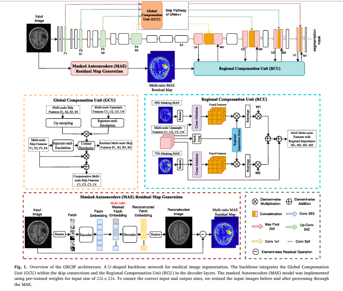
GRCSF sits on top of a UNet++ backbone and adds two new pieces, a Global Compensation Unit inside the skip connections of the encoder, and a Regional Compensation Unit inside the decoder. Think of the first as repairing what downsampling breaks, and the second as pointing the network toward where a lesion is statistically likely to be.
The Global Compensation Unit
Every time the encoder downsamples a feature map, some pixel level information is lost. The Global Compensation Unit tries to quantify exactly how much was lost and where. It takes the downsampled feature map, upsamples it back to the resolution of the previous encoder layer, and compares that reconstructed version against the original skip feature at that layer. The comparison is a pixel wise cosine similarity, refined through a Squeeze and Excitation attention mechanism that highlights the regions most affected by the loss and suppresses the ones that were not.
The output is two things, a residual map that flags where information changed the most, and an updated skip feature that folds that residual back into the original signal before it reaches the decoder. Applied at every layer of UNet++, this creates a chain where each skip connection carries forward not just its own features but an accumulated memory of what earlier layers lost. The authors note that for a simpler architecture like plain U Net, only the updated feature is needed, because there is a single skip path rather than the nested structure UNet++ uses.
The Regional Compensation Unit and the residual maps that guide it
This is where the masked autoencoder comes back into play, and it is the more novel half of the paper. Before segmentation even begins, a pretrained masked autoencoder processes each input scan twice, once with 50 percent of its patches masked and once with 75 percent masked. The 75 percent ratio is the default, and the 50 percent ratio was added to capture more surrounding context. For each masking ratio, the reconstruction is repeated five times to smooth out the randomness of which patches happen to get masked, then averaged. The final residual map is simply the pixel wise absolute difference between the original scan and its averaged reconstruction.
The intuition is straightforward once you sit with it. A masked autoencoder trained on a large set of non lesion slices learns what typical anatomy looks like. When it tries to reconstruct a region that contains an abnormal structure, a stroke lesion, a tumor, a calcification, it tends to reconstruct that region poorly, because nothing in its training resembled it closely. The resulting error, the residual, clusters around exactly the regions a clinician would want flagged.
The Regional Compensation Unit takes these residual maps and the decoder’s own upsampled features, splits both into patches, and runs a cross attention mechanism between them. In parallel, a small scoring module looks only at the decoder features and estimates how likely each patch is to contain a lesion, since a scan can have zero, one or several lesion regions. The cross attended features are then scaled by that importance score and combined with the original decoder features through two learnable weights, one for each masking ratio’s residual map. The result replaces the standard upsampled feature at that decoder layer, carrying forward both the raw imaging signal and the reconstruction based hint about where to look.
Here \(RM_1’\) and \(RM_2’\) are the patch versions of the two residual maps, \(U’\) is the patched decoder feature, \(\varphi\) rearranges patches back into the full feature map, \(\phi\) is the importance scoring function, and \(W_1\) and \(W_2\) are learnable weights balancing the two masking ratios. It is a fairly compact equation for something that is doing a lot of work, blending two independent self supervised signals with the network’s own learned attention.
This second equation describes the Global Compensation Unit’s updated skip feature, where CS is pixel wise cosine similarity, SE is the Squeeze and Excitation attention block, \(RU\) is the re upsampled feature, \(F\) is the original skip feature and \(U\) is the corresponding decoder feature. Both modules follow the same underlying logic, measure a gap, weight it by attention, and fold the correction back into the main signal rather than discarding it.
Why this matters
Most self supervised methods in medical imaging stop at pretraining. GRCSF is, by the authors’ own account, the first segmentation framework to keep the masked autoencoder’s reconstruction error alive as a guidance signal during inference, rather than throwing it away once the weights are initialized.
Three datasets, three very different failure modes
The team tested GRCSF on three public datasets chosen specifically because each one stresses a different weakness in existing segmentation models.
ATLAS version 2.0 provided 655 publicly available cases of T1 weighted brain MRI with manually traced stroke lesion masks, drawn from 33 research cohorts across 20 institutions worldwide. The scans were annotated using ITK SNAP by trained annotators under neuroradiologist guidance, with each lesion traced twice for consistency. To test how well GRCSF generalizes across scanners and imaging protocols, the researchers split the data into four subsets by cohort, so that a model trained on some hospitals’ scans was tested on entirely different hospitals’ scans within each subset.
The MSD Lung Tumor dataset contributed thin section chest CT scans from patients with non small cell lung cancer, sourced from The Cancer Imaging Archive. The team used 64 cases with publicly available ground truth, splitting them into 43 for training, 11 for validation and 10 for testing, with in plane resolution ranging from 0.60 to 0.98 millimeters.
The orCaScore dataset, built for the MICCAI 2014 Challenge on Automatic Coronary Calcium Scoring, added non contrast, ECG triggered cardiac CT scans from 72 patients across four European hospitals, with calcifications manually annotated by an experienced radiologist and a physician. Because ground truth masks exist only for the training portion of the original challenge split, the team carved their own training, validation and held out test patient from those 32 labeled cases, then evaluated against the official 40 patient online test set through the challenge’s own evaluation protocol.
What the numbers actually show
Across ten comparison methods including UNet, UNet++, DeepLabv3, SwinUNet, TransUNet, SPiN, TransFuse, UTNet and the zero shot Segment Anything Model, GRCSF came out ahead on the headline metrics for all three datasets, though not by identical margins and not on every single measure.
| Dataset | Metric | Best prior method | GRCSF |
|---|---|---|---|
| ATLAS stroke lesions | Dice | DeepLabv3, 0.395 | 0.422 |
| ATLAS stroke lesions | IoU | TransUNet, 0.304 | 0.319 |
| MSD lung tumor | Dice | SAM, 0.722 | 0.730 |
| MSD lung tumor | IoU | SAM, 0.583 | 0.583, tied |
| orCaScore, post processed | F1 volume | UNet++, 0.937 | 0.946 |
A few details are worth sitting with rather than skimming past. On the ATLAS dataset, GRCSF held the second best precision and recall scores rather than the top ones, which the authors read as evidence of balanced segmentation, a model that neither over segments nor under segments aggressively, even though its Dice and IoU still led the field because those metrics reward that balance. On the MSD Lung Tumor set, GRCSF posted the lowest false positive rate among all ten methods, a meaningful result for a lesion type where over segmentation is a common failure. And in the orCaScore results without post processing, GRCSF showed its clearest advantage, correctly picking out small calcifications while the standard clinical post processing step, which discards pixels below 130 Hounsfield units, was flattering some of the weaker methods by cleaning up their over segmentation after the fact.
Segment Anything is the interesting outlier in this comparison. Run in a zero shot setting using bounding boxes derived from UNet++ predictions, it edged out GRCSF on MSD Lung Tumor IoU and came close on Dice, benefiting from the higher contrast and more regular shape of lung tumors compared to stroke lesions. But on ATLAS, the same prompting strategy left SAM behind UNet++ itself, because SAM has no way to correct a bounding box that falls entirely inside a false positive region, and low contrast brain lesions produce exactly that kind of unreliable prompt.
GRCSF effectively addresses the limitations of the above mentioned methods in challenging lesion segmentation tasks. It significantly improves sensitivity to small and low contrast lesions by feature compensation. Wang, Chen, Yang and Kim, Pattern Recognition, 2026
What the ablation study reveals about which piece is doing the work
The most useful table in the paper for anyone trying to decide whether to adopt this approach is the ablation study on ATLAS, because it isolates each component’s contribution rather than just reporting the final number.
| Configuration | Dice | IoU | Precision | Recall |
|---|---|---|---|---|
| UNet++ baseline | 0.381 | 0.286 | 0.476 | 0.409 |
| Add Global Compensation Unit only | 0.394 | 0.294 | 0.485 | 0.426 |
| Add cross attention with residual maps, no importance score | 0.408 | 0.306 | 0.478 | 0.439 |
| Full GRCSF, including importance scoring | 0.422 | 0.319 | 0.497 | 0.451 |
Each addition moves the needle, and none of the three components is doing all the work alone. The Global Compensation Unit alone lifted Dice by about 1.3 percentage points over the baseline. Adding residual map guidance through cross attention added roughly another 1.4 points. Adding the patch level importance scoring on top of that added a further 1.4 points. Recall improved at every stage too, which matters clinically, since a missed lesion is generally a more serious error than a slightly over drawn one.
The researchers also tested a series of alternative design choices, and the results are frank about what did not work. Swapping the Squeeze and Excitation block for a spatial attention module did not help. Replacing the Global Compensation Unit with pyramidal attention or attention gated skip connections underperformed the original design. Replacing the masked autoencoder residual map with a Grad CAM saliency map from a plain UNet dropped Dice sharply, to 0.476, showing that the reconstruction based signal is doing something a simple gradient based saliency map cannot replicate. Swapping in a lightweight MobileNet encoder in place of the UNet++ backbone also hurt performance substantially, which tells you this is not a framework you can casually shrink for speed without giving something up.
A practical detail for anyone reproducing this
The paper found that averaging five separate masked autoencoder reconstructions per masking ratio, rather than using a single reconstruction, improved Dice from 0.520 to 0.581 on their tuning subset, at a cost of roughly eighteen extra seconds per patient. Using both the 50 percent and 75 percent masking ratios together also beat either ratio used alone.
The clinical translation gap
It is worth being direct about the distance between what this paper demonstrates and what a hospital could deploy tomorrow. GRCSF was trained and tested on retrospective, publicly available research datasets with careful, expert generated annotations, not on a live clinical pipeline with the messiness of real acquisition variability, incomplete scans, or patients with multiple comorbidities complicating the imaging. The ATLAS dataset in particular was deliberately split so that test patients came from different research cohorts and scanner types than the training patients, which is a genuinely useful stress test for generalization, but it is still a research split, not a deployment across new hospitals with new equipment and new patient populations that the model has never seen in any form.
Runtime is the other practical constraint. The full GRCSF pipeline, including residual map generation, took about 26 seconds per patient on the ATLAS dataset and about 62 seconds per patient on the MSD Lung Tumor dataset, on a single NVIDIA RTX A6000 Ada GPU. That is fast enough for research benchmarking and plausible for a batch reading workflow, but it is meaningfully slower than the fastest baseline in the comparison, plain UNet, by roughly 24 and 36 seconds respectively. Whether that overhead is acceptable depends entirely on the clinical workflow it would sit inside, and the paper does not claim to have tested that question.
None of this diminishes the technical contribution, but it does mean the honest reading of this paper is a strong result on curated benchmarks and a real research advance in method design, not a validated clinical product.
Honest limitations
The authors are candid about where GRCSF falls short. The computational cost, driven mostly by the five times repeated masked autoencoder reconstruction across two masking ratios, is the headline limitation they name directly, and they specifically flag it as a barrier to large scale deployment or routine clinical use in its current form. Sample sizes across all three datasets are modest by deep learning standards, 655 patients for ATLAS, 64 for MSD Lung Tumor and 72 for orCaScore, which is typical for specialized medical imaging research but still leaves open questions about performance on rarer lesion presentations that a larger dataset might surface. The orCaScore evaluation also relies on a post processing step, discarding pixels below 130 Hounsfield units, that is standard practice in coronary calcium scoring but does mean the officially reported metrics are not a pure measure of the raw segmentation output, a point the authors address directly by also reporting results without that step.
Model size sits in an odd middle zone too. At 42.85 million parameters, GRCSF is heavier than UNet or DeepLabv3 but notably lighter than TransUNet at over 93 million or TransFuse at over 143 million, and its peak memory use of 690 megabytes is actually lower than several of the transformer based competitors. The tradeoff is real but it is not simply worse across the board, it is a different set of costs concentrated in the residual map generation step rather than in the backbone itself.
Conclusion
The core achievement of this paper is a demonstration that a masked autoencoder’s reconstruction error, usually discarded once pretraining finishes, can be repurposed as a live guidance signal that meaningfully improves segmentation of exactly the lesions that give existing methods the most trouble. Across three genuinely different imaging problems, an isointense brain lesion on MRI, an irregular tumor on chest CT, and a tiny calcification on cardiac CT, the same two added modules produced consistent gains over ten established comparison methods, which is a stronger form of evidence than a single dataset win would be.
The conceptual shift matters beyond this particular architecture. Self supervised learning in medical imaging has largely been treated as a warm up act, a way to get better starting weights before the real supervised training begins. GRCSF’s framing, keep the reconstruction process running and let its errors point toward anomalies, suggests a broader pattern that other segmentation frameworks could borrow even without adopting the specific Global and Regional Compensation Unit design described here.
That transferability seems genuine rather than aspirational. The authors note explicitly that both compensation units can be integrated into any U shaped convolutional backbone that uses skip connections, not just UNet++, and the ablation study’s finding that a Grad CAM based alternative performed far worse than the masked autoencoder residual map is a useful negative result for anyone tempted to substitute a cheaper saliency method.
The honest remaining limitations, computational overhead, modest dataset sizes, and an unresolved gap between benchmark performance and clinical deployment, are not small asterisks. They are the actual next research agenda, and the authors say as much, pointing toward more targeted masking strategies and lighter backbones as the obvious next steps rather than claiming the current version is deployment ready.
Read against the wider field, this paper is less about beating a leaderboard and more about making a specific, testable claim, that reconstruction error from self supervised pretraining still has information left in it once training ends, and that information is worth the extra seconds it costs to extract. The three dataset result makes that claim harder to dismiss than a single win would, and it leaves a clear, well marked trail for the next team that wants to push the idea further.
A working PyTorch implementation
The block below is a full, runnable implementation of the two core modules described in the paper, the Global Compensation Unit and the Regional Compensation Unit, wired into a small UNet style backbone with a combined Dice and focal loss, a training loop, an evaluation function and a smoke test on random dummy data. It is written to make the mechanics concrete rather than to reproduce the paper’s exact benchmark numbers, which required the specific UNet++ backbone, a pretrained ViT Large masked autoencoder, and the full ATLAS, MSD and orCaScore datasets.
# grcsf_reference.py
# A compact, runnable reference implementation of the Global Compensation Unit (GCU)
# and Regional Compensation Unit (RCU) from Wang, Chen, Yang and Kim, Pattern Recognition 2026.
# This is an educational reference, not a reproduction of the paper's exact backbone or datasets.

import torch
import torch.nn as nn
import torch.nn.functional as F


class SqueezeExcite(nn.Module):
    """Channel attention block used inside the Global Compensation Unit."""

    def __init__(self, channels, reduction=8):
        super().__init__()
        hidden = max(channels // reduction, 4)
        self.pool = nn.AdaptiveAvgPool2d(1)
        self.fc = nn.Sequential(
            nn.Linear(channels, hidden),
            nn.ReLU(inplace=True),
            nn.Linear(hidden, channels),
            nn.Sigmoid(),
        )

    def forward(self, x):
        b, c, _, _ = x.shape
        weights = self.pool(x).view(b, c)
        weights = self.fc(weights).view(b, c, 1, 1)
        return x * weights


class GlobalCompensationUnit(nn.Module):
    """
    Recovers pixel level detail lost during downsampling.
    Compares a re upsampled downsampled feature map against the original skip
    feature using pixel wise cosine similarity, then folds the difference back
    into the skip feature before it reaches the decoder.
    """

    def __init__(self, channels):
        super().__init__()
        self.se_f = SqueezeExcite(channels)
        self.se_u = SqueezeExcite(channels)

    def forward(self, downsampled_feature, skip_feature, decoder_feature):
        # downsampled_feature: S, from deeper encoder layer
        # skip_feature: F, at this encoder layer
        # decoder_feature: U, the matching decoder layer feature
        re_up = F.interpolate(
            downsampled_feature, size=skip_feature.shape[-2:], mode="bilinear", align_corners=False
        )
        se_f = self.se_f(skip_feature)
        se_u = self.se_u(decoder_feature)

        gated_up = re_up * se_u
        cos_sim = F.cosine_similarity(gated_up, se_f, dim=1, eps=1e-6).unsqueeze(1)

        residual_map = cos_sim
        updated_skip = residual_map * skip_feature + skip_feature
        return updated_skip, residual_map


class PatchCrossAttention(nn.Module):
    """Cross attention between a patched residual map and patched decoder features."""

    def __init__(self, in_channels, feat_channels, patch_size):
        super().__init__()
        self.patch_size = patch_size
        self.query_proj = nn.Conv2d(in_channels, feat_channels, kernel_size=1)
        self.key_proj = nn.Conv2d(feat_channels, feat_channels, kernel_size=1)
        self.value_proj = nn.Conv2d(feat_channels, feat_channels, kernel_size=1)
        self.out_proj = nn.Conv2d(feat_channels, feat_channels, kernel_size=1)

    def forward(self, residual_map, decoder_feature):
        p = self.patch_size
        residual_resized = F.interpolate(
            residual_map, size=decoder_feature.shape[-2:], mode="bilinear", align_corners=False
        )
        q = self.query_proj(residual_resized)
        k = self.key_proj(decoder_feature)
        v = self.value_proj(decoder_feature)

        b, c, h, w = q.shape
        q = q.unfold(2, p, p).unfold(3, p, p).reshape(b, c, -1, p * p)
        k = k.unfold(2, p, p).unfold(3, p, p).reshape(b, c, -1, p * p)
        v = v.unfold(2, p, p).unfold(3, p, p).reshape(b, c, -1, p * p)

        attn = torch.einsum("bcnp,bcnq->bnpq", q, k) / (c ** 0.5)
        attn = F.softmax(attn, dim=-1)
        fused = torch.einsum("bnpq,bcnq->bcnp", attn, v)

        n_patches_h = h // p
        n_patches_w = w // p
        fused = fused.reshape(b, c, n_patches_h, n_patches_w, p, p)
        fused = fused.permute(0, 1, 2, 4, 3, 5).reshape(b, c, h, w)
        return self.out_proj(fused)


class ImportanceScorer(nn.Module):
    """Estimates the patch level likelihood that a region contains a lesion."""

    def __init__(self, channels, patch_size):
        super().__init__()
        self.patch_size = patch_size
        self.conv = nn.Conv2d(channels, channels, kernel_size=1)
        hidden = max(channels // 2, 8)
        self.mlp = nn.Sequential(
            nn.Linear(channels, hidden),
            nn.ReLU(inplace=True),
            nn.Linear(hidden, hidden),
            nn.ReLU(inplace=True),
            nn.Linear(hidden, 1),
            nn.Sigmoid(),
        )

    def forward(self, decoder_feature):
        p = self.patch_size
        x = self.conv(decoder_feature)
        b, c, h, w = x.shape
        patches = x.unfold(2, p, p).unfold(3, p, p)
        patches = patches.mean(dim=(-1, -2))
        scores = self.mlp(patches.permute(0, 2, 3, 1))
        scores = scores.permute(0, 3, 1, 2)
        scores = F.interpolate(scores, size=(h, w), mode="nearest")
        return scores


class RegionalCompensationUnit(nn.Module):
    """
    Fuses two masked autoencoder residual maps with decoder features using
    patch based cross attention and a learned importance score, following
    Equation 6 of the paper.
    """

    def __init__(self, feat_channels, patch_size):
        super().__init__()
        self.attn_50 = PatchCrossAttention(1, feat_channels, patch_size)
        self.attn_75 = PatchCrossAttention(1, feat_channels, patch_size)
        self.importance = ImportanceScorer(feat_channels, patch_size)
        self.w1 = nn.Parameter(torch.tensor(0.5))
        self.w2 = nn.Parameter(torch.tensor(0.5))

    def forward(self, residual_50, residual_75, decoder_feature):
        importance = self.importance(decoder_feature)
        fused_50 = self.attn_50(residual_50, decoder_feature) * importance
        fused_75 = self.attn_75(residual_75, decoder_feature) * importance
        weighted = fused_50 * self.w1 + fused_75 * self.w2
        return weighted + decoder_feature


class ConvBlock(nn.Module):
    def __init__(self, in_ch, out_ch):
        super().__init__()
        self.block = nn.Sequential(
            nn.Conv2d(in_ch, out_ch, 3, padding=1),
            nn.BatchNorm2d(out_ch),
            nn.ReLU(inplace=True),
            nn.Conv2d(out_ch, out_ch, 3, padding=1),
            nn.BatchNorm2d(out_ch),
            nn.ReLU(inplace=True),
        )

    def forward(self, x):
        return self.block(x)


class GRCSFLite(nn.Module):
    """
    A small four level U shaped backbone with a Global Compensation Unit at
    every skip connection and a Regional Compensation Unit at the final two
    decoder levels, matching the spirit of the paper's design at a scale
    that is easy to run and inspect.
    """

    def __init__(self, in_channels=1, base_channels=16, patch_size=8):
        super().__init__()
        c1, c2, c3, c4 = base_channels, base_channels * 2, base_channels * 4, base_channels * 8

        self.enc1 = ConvBlock(in_channels, c1)
        self.enc2 = ConvBlock(c1, c2)
        self.enc3 = ConvBlock(c2, c3)
        self.bottleneck = ConvBlock(c3, c4)

        self.pool = nn.MaxPool2d(2)

        self.up3 = nn.ConvTranspose2d(c4, c3, 2, stride=2)
        self.dec3 = ConvBlock(c3 * 2, c3)
        self.up2 = nn.ConvTranspose2d(c3, c2, 2, stride=2)
        self.dec2 = ConvBlock(c2 * 2, c2)
        self.up1 = nn.ConvTranspose2d(c2, c1, 2, stride=2)
        self.dec1 = ConvBlock(c1 * 2, c1)

        self.gcu3 = GlobalCompensationUnit(c3)
        self.gcu2 = GlobalCompensationUnit(c2)
        self.gcu1 = GlobalCompensationUnit(c1)

        self.rcu2 = RegionalCompensationUnit(c2, patch_size)
        self.rcu1 = RegionalCompensationUnit(c1, patch_size)

        self.head = nn.Conv2d(c1, 1, kernel_size=1)

    def forward(self, image, residual_50, residual_75):
        e1 = self.enc1(image)
        e2 = self.enc2(self.pool(e1))
        e3 = self.enc3(self.pool(e2))
        b = self.bottleneck(self.pool(e3))

        u3 = self.up3(b)
        s3, _ = self.gcu3(b, e3, u3)
        d3 = self.dec3(torch.cat([u3, s3], dim=1))

        u2 = self.up2(d3)
        s2, _ = self.gcu2(d3, e2, u2)
        d2_in = self.rcu2(residual_50, residual_75, u2)
        d2 = self.dec2(torch.cat([d2_in, s2], dim=1))

        u1 = self.up1(d2)
        s1, _ = self.gcu1(d2, e1, u1)
        d1_in = self.rcu1(residual_50, residual_75, u1)
        d1 = self.dec1(torch.cat([d1_in, s1], dim=1))

        return self.head(d1)


def dice_loss(pred, target, eps=1e-6):
    pred = torch.sigmoid(pred)
    intersection = (pred * target).sum(dim=(1, 2, 3))
    union = pred.sum(dim=(1, 2, 3)) + target.sum(dim=(1, 2, 3))
    return 1 - ((2 * intersection + eps) / (union + eps)).mean()


def focal_loss(pred, target, alpha=0.25, gamma=2.0, eps=1e-6):
    prob = torch.sigmoid(pred)
    pt = torch.where(target == 1, prob, 1 - prob).clamp(min=eps, max=1 - eps)
    weight = alpha * (1 - pt) ** gamma
    loss = -weight * torch.log(pt)
    return loss.mean()


def grcsf_loss(pred, target):
    # Matches the mixed dice and focal loss used for ATLAS and MSD Lung Tumor.
    return dice_loss(pred, target) + focal_loss(pred, target)


def make_residual_maps(image, mask_ratio, noise_scale=0.15):
    """
    Stand in for a real masked autoencoder pass. In the paper this is the
    pixel wise absolute difference between the input image and the average
    of five masked autoencoder reconstructions. Swap this for a real
    pretrained masked autoencoder in a full training run.
    """
    mask = (torch.rand_like(image) > mask_ratio).float()
    noisy_reconstruction = image * mask + torch.randn_like(image) * noise_scale
    residual = torch.abs(image - noisy_reconstruction)
    return residual


def train_one_epoch(model, optimizer, images, masks, device):
    model.train()
    residual_50 = make_residual_maps(images, mask_ratio=0.5).to(device)
    residual_75 = make_residual_maps(images, mask_ratio=0.75).to(device)

    optimizer.zero_grad()
    pred = model(images, residual_50, residual_75)
    loss = grcsf_loss(pred, masks)
    loss.backward()
    optimizer.step()
    return loss.item()


@torch.no_grad()
def evaluate(model, images, masks, device, threshold=0.5):
    model.eval()
    residual_50 = make_residual_maps(images, mask_ratio=0.5).to(device)
    residual_75 = make_residual_maps(images, mask_ratio=0.75).to(device)

    logits = model(images, residual_50, residual_75)
    prob = torch.sigmoid(logits)
    pred_mask = (prob > threshold).float()

    intersection = (pred_mask * masks).sum()
    union = pred_mask.sum() + masks.sum()
    dice = (2 * intersection + 1e-6) / (union + 1e-6)
    return dice.item()


def smoke_test():
    """Runs one training step and one evaluation step on random dummy data."""
    device = torch.device("cuda" if torch.cuda.is_available() else "cpu")
    torch.manual_seed(0)

    batch_size, height, width = 2, 128, 128
    images = torch.rand(batch_size, 1, height, width, device=device)
    masks = (torch.rand(batch_size, 1, height, width, device=device) > 0.9).float()

    model = GRCSFLite(in_channels=1, base_channels=16, patch_size=8).to(device)
    optimizer = torch.optim.Adam(model.parameters(), lr=1e-4)

    train_loss = train_one_epoch(model, optimizer, images, masks, device)
    dice_score = evaluate(model, images, masks, device)

    print(f"Smoke test training loss {train_loss:.4f}")
    print(f"Smoke test dice score {dice_score:.4f}")
    assert torch.isfinite(torch.tensor(train_loss))
    print("Smoke test passed")


if __name__ == "__main__":
    smoke_test()
Frequently asked questions
What does GRCSF stand for and what problem does it solve
GRCSF stands for the Global and Regional Compensation Segmentation Framework. It targets lesions that are hard to segment because they are small, low contrast or irregularly shaped, by recovering global detail lost during downsampling and by using masked autoencoder reconstruction error to guide the network toward likely lesion regions.
Is GRCSF a replacement for a radiologist
No. It is a research segmentation method evaluated on retrospective public datasets. Nothing in the paper claims diagnostic authority, and any clinical use would need separate validation, regulatory clearance and oversight by qualified professionals.
What makes the masked autoencoder residual map different from a normal saliency map
A saliency map like Grad CAM highlights regions that influenced a trained classifier’s decision. The residual map here comes from an unsupervised reconstruction process. It flags regions the masked autoencoder could not reconstruct well because they did not resemble the typical anatomy it learned from unlabeled scans. The paper’s ablation study found the reconstruction based residual map outperformed a Grad CAM alternative by a wide margin, 0.581 Dice compared with 0.476.
How much slower is GRCSF than a standard UNet
On the datasets tested, the full pipeline added roughly 24 seconds per patient on ATLAS and roughly 36 seconds per patient on the MSD Lung Tumor dataset compared with plain UNet, mostly from generating the masked autoencoder residual maps. Total time per patient was under one minute on a single high end GPU.
Can these two modules be added to other segmentation backbones
The authors state that the Global Compensation Unit and Regional Compensation Unit can be integrated into any U shaped convolutional architecture that uses skip connections, not only UNet++, though the paper’s own experiments use UNet++ as the backbone throughout.
Which datasets were used to test the method
Three public datasets. ATLAS version 2.0 for brain stroke lesions on T1 weighted MRI, the Medical Segmentation Decathlon Lung Tumor set for non small cell lung cancer on chest CT, and orCaScore for coronary artery calcification on non contrast cardiac CT.
Read the full paper for the complete equations, all ten comparison methods and every ablation table.
Read the paper on Pattern Recognition orCaScore evaluation frameworkRelated reading
Academic citation. Wang, C., Chen, Z., Yang, J. Y. H. and Kim, J. Improving lesion segmentation in medical images by global and regional feature compensation. Pattern Recognition, 172, 112461, 2026. https://doi.org/10.1016/j.patcog.2025.112461
This analysis is based on the published paper and an independent evaluation of its claims.
Thanks for sharing. I read many of your blog posts, cool, your blog is very good. https://www.binance.com/pt-BR/register?ref=GJY4VW8W