
Key points
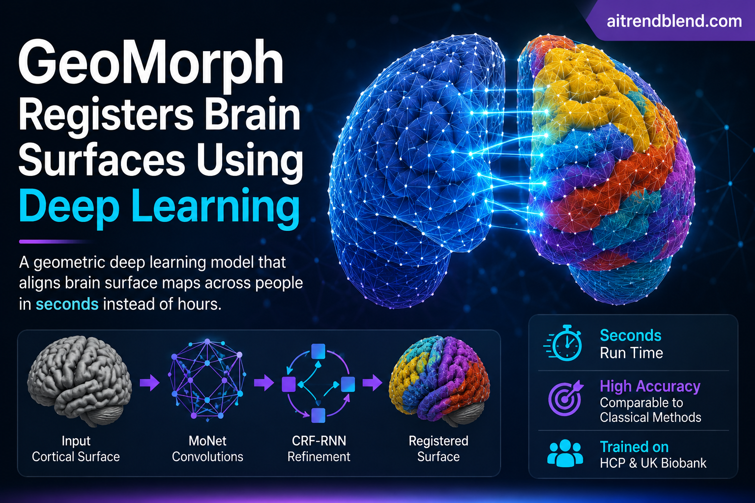
- GeoMorph is a geometric deep learning model that aligns cortical surface meshes by learning displacements for a small grid of control points, then choosing from a set of candidate target locations.
- It separates two jobs that earlier deep learning approaches folded together, extracting features from each brain first, then registering the extracted features, rather than mixing the two.
- A conditional random field, run through a recurrent network, smooths the deformation so neighboring control points move in a coordinated way instead of independently.
- On sulcal depth alignment it lands just behind Spherical Demons and ahead of Multimodal Surface Matching for distortion, while running in about eight seconds instead of thirteen minutes to one hour.
- On multimodal alignment using myelin and resting state functional maps, it matches the classical tool MSMAll on similarity while finishing in roughly seven seconds against one and a half hours.
- The code and trained weights are public, and the authors are candid about where diffeomorphism guarantees and rotational equivariance are still missing.
Why lining up two brains is harder than it sounds
Every cortex is folded in its own particular way. The overall pattern of ridges and grooves, called gyri and sulci, is recognizable from one person to the next, but the exact shape, depth, and location of any given fold varies quite a bit. Neuroscience has learned to work around this by mapping each individual brain onto a shared, inflated sphere and then registering that sphere to a group average template. Once every brain sits in the same coordinate space, a researcher can average functional activity across a hundred people, build a population atlas, or test whether a particular region differs between two groups.
For a long time, that registration step was driven by folding patterns alone, things like sulcal depth or average curvature. Freesurfer works this way, minimizing the difference between an individual’s convexity map and the population average first described by Fischl and colleagues in 1999. Spherical Demons later sped this up with a diffeomorphic approach borrowed from classical image registration. Multimodal Surface Matching, or MSM, went further and treated registration as a discrete labeling problem, which made it flexible about what similarity measure to optimize and more robust to noisy data and local minima.
The catch is that folding patterns are a weak proxy for where a cortical area actually is. Studies comparing folding based alignment to alignment driven by function or myelin content have shown that some regions simply do not sit in a consistent spot relative to the folds. That pushed the field toward multimodal registration, matching resting state functional networks and T1 weighted to T2 weighted myelin maps directly, since these correlate more tightly with the true boundaries of cortical areas. MSMAll, the multimodal version used across the Human Connectome Project, does exactly this, and it works well, but it is expensive, taking up to an hour and a half per subject on a CPU.
What GeoMorph actually does differently
GeoMorph is built around three ideas stacked on top of each other. First, it learns separate feature representations for the moving brain and the fixed template using a series of graph convolutions. Second, it treats registration as a discrete choice problem, where a coarse grid of control points on the moving sphere is deformed toward one of a fixed set of candidate label locations. Third, it smooths that choice with a conditional random field so neighboring control points do not drift apart in incompatible directions.
Feature extraction on a sphere
Because cortical surfaces do not have a natural grid the way an image does, GeoMorph uses MoNet convolutions, a graph convolution scheme originally proposed by Monti and colleagues that defines a learnable Gaussian kernel over the local coordinates of a vertex’s neighbors. Each neighbor y of a point x gets a pseudo coordinate describing its position relative to x, and the kernel weight is a Gaussian function of that coordinate.
The Gaussian weighting function itself has a learnable mean and covariance per kernel.
The moving and fixed surfaces each pass through their own stack of these convolutional blocks, so the network can pick up whatever quirks show up in a given input, sparse functional noise on one side, smoother myelin gradients on the other. Only the last two blocks share weights across the two paths, which nudges the high level features toward a common, spatially aligned representation while still letting the early layers stay specialized. That separation matters more here than in earlier single path designs such as the authors’ own prior model, DDR, because multimodal inputs bring very different noise profiles that benefit from dedicated early processing.
Choosing a displacement as a classification problem
Once features are extracted, a series of ResNet style blocks produces a score for every candidate label point around each control point. A softmax turns those scores into probabilities, and the expected displacement is read off from the highest probability label. This is the same basic idea as MSM’s discrete optimization, but instead of solving a combinatorial labeling problem at inference time, GeoMorph learns a function that predicts the labeling directly, which is why it is so much faster to run once trained.
Smoothing the deformation with a CRF that thinks like an RNN
A classifier working on its own would let every control point move independently, which the authors show leads to distorted, badly behaved deformations. To fix that, GeoMorph borrows an idea from semantic segmentation, the CRF as RNN formulation introduced by Zheng and colleagues in 2015, and adapts it to run over the control point graph. The cost function being minimized combines the unary cost of each individual assignment with a pairwise cost that penalizes neighboring points choosing very different displacements.
The pairwise term is a learnable compatibility function combined with a Gaussian kernel over the label locations, and the whole thing is optimized with five iterations of mean field inference, unrolled as a small recurrent network so gradients flow through it during training. It is a neat trick because it turns a classic probabilistic graphical model into something that trains end to end with ordinary backpropagation, without ever explicitly solving the CRF at inference time.
The practical effect is that GeoMorph gets discrete optimization’s robustness to noise and local minima, MSM’s original selling point, without paying MSM’s runtime cost, because the expensive combinatorial search happens once during training rather than for every new brain at inference time.
How well does it actually work
The authors tested GeoMorph on two large datasets, 1,110 adults from the Human Connectome Project and 3,000 UK Biobank participants, and compared it against Freesurfer, Spherical Demons, two versions of MSM, and a competing deep learning method called S3Reg. For univariate alignment using only sulcal depth, they report cross correlation similarity alongside areal and shape distortion, which measure how much a triangle on the mesh gets stretched or sheared by the deformation.
| Method | Areal distortion, 95th percentile | Shape distortion, 95th percentile | Typical run time |
|---|---|---|---|
| Spherical Demons | 0.50 | 0.50 | about 1 minute, CPU |
| GeoMorph | 0.53 | 0.63 | about 8 seconds, GPU |
| MSM Strain | 0.53 | 1.17 | about 1 hour, CPU |
| Freesurfer | 0.82 | 1.29 | about 30 minutes, CPU |
| MSM Pair | 1.24 | 1.61 | about 13 minutes, CPU |
| S3Reg | 0.82 | 1.35 | about 9 seconds, GPU |
Spherical Demons still edges out GeoMorph on pure distortion, and that is worth saying plainly rather than smoothing over. But GeoMorph beats MSM Strain, the more heavily regularized version of MSM, and comfortably beats MSM Pair, Freesurfer, and S3Reg on both distortion measures, while running roughly two orders of magnitude faster than any of the classical CPU based methods.
The more interesting test is multimodal registration, aligning myelin maps and resting state network maps together, which is what actually matters for locating functional areas precisely. Here GeoMorph is compared against MSMAll, the gold standard multimodal pipeline used across the Human Connectome Project.
| Dataset and method | Myelin similarity | Functional similarity | Run time |
|---|---|---|---|
| HCP, MSMAll | 0.945 | 0.566 | about 1.5 hours, CPU |
| HCP, GeoMorphAll | 0.975 | 0.569 | about 7.7 seconds, GPU |
| UK Biobank, MSMAll | 0.944 | 0.40 | about 1.5 hours, CPU |
| UK Biobank, GeoMorphAll | 0.96 | 0.40 | about 7.7 seconds, GPU |
GeoMorphAll slightly edges out MSMAll on myelin similarity and lands essentially even on the functional similarity measure, on both datasets. That is a meaningful result because MSM was tuned specifically on Human Connectome Project style data, so holding up equally well on the UK Biobank cohort, which was scanned with different hardware and a shorter functional protocol, says something about how well the learned features generalize rather than just memorizing one acquisition’s quirks.
The paper backs this up with an independent check that did not feed into training at all. Using task fMRI data from seven Human Connectome Project tasks, ranging from emotion processing to working memory, the authors measured cluster mass, a statistic that rewards larger and more strongly activated regions in group level activation maps. GeoMorphAll produced higher cluster mass than the unimodal, folding only alignment in every one of the seven tasks, tracking MSMAll closely across the board, which is the kind of downstream validation that actually matters more than the registration metric itself.
What the ablations reveal
The authors did not just report headline numbers, they took the model apart piece by piece. Removing the CRF RNN network barely changed the cross correlation similarity score but noticeably worsened every distortion measure, confirming that the smoothing step earns its keep even though it is not the thing directly being optimized for accuracy. Swapping the CRF RNN for a continuous velocity field with scaling and squaring layers, the more common way of enforcing smooth deformations in the wider registration literature, produced clearly worse results on both similarity and distortion, which is a genuinely useful finding for anyone building a competing architecture. And replacing the twin path feature extraction network with a single shared path, the design used in the authors’ earlier DDR model, made distortion worse across every metric tested, confirming that separating the moving and fixed feature paths was not a cosmetic choice.
Where this fits in the bigger picture
Cortical surface registration sits upstream of a lot of neuroscience. Every study that reports group average activation maps, builds a cortical parcellation, or compares patient and control groups is leaning on a registration step somewhere in the pipeline. A tool that runs in seconds instead of an hour and a half changes what is practically possible. Building population specific templates conditioned on age or diagnosis, running registration as part of an interactive analysis pipeline, or processing biobank scale cohorts with tens of thousands of participants all become far more tractable when each subject costs seconds of GPU time rather than a CPU hour.
It is also part of a broader shift in how the geometric deep learning field is approaching non Euclidean data. Convolutional networks are extremely well understood on regular pixel grids, but a folded cortical sphere, like a molecule, a social graph, or a 3D mesh, does not have that regular structure. MoNet, the convolution scheme GeoMorph relies on, along with related graph attention and spherical CNN approaches, is part of a wider effort to bring the inductive biases that made convolutional networks so effective on images to domains where there is no obvious grid to convolve over.
Clinical translation gap
It is worth being direct about the distance between this result and anything resembling clinical deployment. GeoMorph was trained and evaluated on healthy adult research cohorts, 1,110 Human Connectome Project participants aged 22 to 35 and 3,000 UK Biobank participants aged 46 to 83. Neither cohort includes patients with the kinds of severe cortical malformation, tumor mass effect, or post surgical anatomy that a clinical registration tool would eventually need to handle. The paper itself flags that achieving good alignment on functional topography is not always possible even in healthy brains, noting that roughly 10 percent of subjects show inconsistent alignment for one particular visual area, a finding drawn from earlier work by Glasser and colleagues. A registration tool intended for surgical planning or individual patient comparison would need dedicated validation on patient populations, ideally with ground truth from an independent source such as intraoperative mapping, before anyone should rely on it outside a research context.
Regulatory and safety notes
GeoMorph is published research software released for academic use, not a cleared or approved medical device. Any tool derived from this work that touched patient care decisions would need to go through the relevant regulatory pathway in its jurisdiction, along with clinical validation studies specific to the intended patient population, before it could be used outside a research setting.
Honest limitations
The authors are candid about several open issues, and it is worth taking them at their word rather than glossing past them for a tidier narrative.
- Memory constraints capped the control point grid at an icosphere of order 4, roughly 2,542 control points, which the paper says limits how much the model’s performance could still improve with a finer grid, based on the resolution ablation in Table 4 of the paper showing steady gains from order 2 to order 4.
- GeoMorph does not explicitly enforce diffeomorphic deformations the way Spherical Demons and MSM do. The authors report that in practice the CRF RNN’s regularization was strong enough that all their results turned out diffeomorphic anyway, but that is an empirical observation from their experiments, not a guarantee built into the architecture.
- MoNet convolutions have shown good empirical robustness to rotation in prior work, but they lack a formal equivariance guarantee, unlike some newer spherical convolution designs. The authors list this as a direction for future versions.
- Because GeoMorph enforces smoothness the way it does, it may struggle with the roughly 10 percent of subjects the paper mentions where true functional alignment requires breaking diffeomorphic assumptions altogether, an open problem the authors describe rather than solve.
- Both training datasets are adult cohorts scanned on Siemens 3 Tesla hardware. Generalization to pediatric brains, different field strengths, or substantially different acquisition protocols was not tested in this paper.
None of this undercuts the core result. It is a useful reminder that fast and accurate on two well curated adult cohorts is a real achievement, and also a specific, bounded one, not a finished clinical tool.
Conclusion
GeoMorph’s core achievement is showing that a discrete, learning based approach to cortical registration can match a heavily engineered classical pipeline, MSMAll, on the metric that actually matters, how well functional and structural landmarks line up across subjects, while cutting run time from an hour and a half to under eight seconds. That is not a marginal speed improvement. It is the difference between registration being a batch job you queue overnight and registration being something you can build into an interactive tool.
The conceptual shift underneath that speed gain is just as interesting as the speed itself. Instead of treating feature extraction and registration as one entangled optimization problem, the way most prior deep learning registration methods did, GeoMorph splits them into a learned feature extractor followed by a learned discrete classifier smoothed by a differentiable CRF. That separation, more than any single architectural trick, seems to be what lets the model handle messy multimodal inputs, sparse functional maps sitting alongside comparatively clean myelin maps, without either signal dragging the other’s alignment off course.
There is a reasonable case that this general pattern, independent per modality feature extraction followed by a shared discrete decision layer, could transfer well beyond brain surfaces. Any registration problem involving multiple noisy, structurally different input channels on a non Euclidean domain, cardiac surface meshes tracked across a cycle, or multi stain histology sections, shares the same basic tension between modality specific noise and a need for a single coherent deformation field.
The honest remaining limitations matter for anyone deciding whether to build on this work today. No enforced diffeomorphism, a control grid capped by memory rather than by a principled stopping point, and convolutions without formal rotational equivariance are all real gaps, and the authors say so themselves rather than papering over them. Anyone adapting GeoMorph for a new anatomical domain or a patient population should treat those as open engineering and validation questions, not settled details.
Cortical registration is one of those unglamorous infrastructure problems that almost nobody outside neuroimaging thinks about, yet nearly every population level finding in the field depends on it working well. A tool that gets close to the best classical method’s accuracy at a small fraction of the compute cost is the kind of unglamorous win that ends up mattering a great deal, quietly, in the background of a hundred other papers that will cite it only as a preprocessing step.
Complete PyTorch implementation and smoke test
The block below is a working, independently written implementation of GeoMorph’s core components, a MoNet style graph convolution, the twin path feature extraction network, the discrete classifier, and the CRF RNN mean field smoothing step, run on a small synthetic icosphere mesh as a smoke test. It is meant to make the architecture concrete, not to reproduce the paper’s full scale results, which were trained on the icosphere order 4 control grid described above using real Human Connectome Project and UK Biobank data.
import math
import torch
import torch.nn as nn
import torch.nn.functional as F

torch.manual_seed(0)

# 1. Icosphere generation, order 0 gives 12 vertices used as control points,
# order 1 gives 42 vertices used as the dense mesh and label space.
def make_icosphere_order0():
    t = (1.0 + 5 ** 0.5) / 2.0
    verts = torch.tensor([
        [-1, t, 0], [1, t, 0], [-1, -t, 0], [1, -t, 0],
        [0, -1, t], [0, 1, t], [0, -1, -t], [0, 1, -t],
        [t, 0, -1], [t, 0, 1], [-t, 0, -1], [-t, 0, 1],
    ], dtype=torch.float32)
    verts = verts / verts.norm(dim=1, keepdim=True)
    faces = torch.tensor([
        [0, 11, 5], [0, 5, 1], [0, 1, 7], [0, 7, 10], [0, 10, 11],
        [1, 5, 9], [5, 11, 4], [11, 10, 2], [10, 7, 6], [7, 1, 8],
        [3, 9, 4], [3, 4, 2], [3, 2, 6], [3, 6, 8], [3, 8, 9],
        [4, 9, 5], [2, 4, 11], [6, 2, 10], [8, 6, 7], [9, 8, 1],
    ], dtype=torch.long)
    return verts, faces


def subdivide(verts, faces):
    mid_cache = {}
    new_verts = verts.tolist()

    def midpoint(i, j):
        key = tuple(sorted((i, j)))
        if key in mid_cache:
            return mid_cache[key]
        v = (verts[i] + verts[j]) / 2.0
        v = v / v.norm()
        new_verts.append(v.tolist())
        idx = len(new_verts) - 1
        mid_cache[key] = idx
        return idx

    new_faces = []
    for f in faces.tolist():
        a, b, c = f
        ab = midpoint(a, b)
        bc = midpoint(b, c)
        ca = midpoint(c, a)
        new_faces += [[a, ab, ca], [b, bc, ab], [c, ca, bc], [ab, bc, ca]]

    return torch.tensor(new_verts, dtype=torch.float32), torch.tensor(new_faces, dtype=torch.long)


def faces_to_neighbors(n_verts, faces):
    nb = [set() for _ in range(n_verts)]
    for a, b, c in faces.tolist():
        nb[a].update([b, c])
        nb[b].update([a, c])
        nb[c].update([a, b])
    return [sorted(list(s)) for s in nb]


ico0_verts, ico0_faces = make_icosphere_order0()
ico1_verts, ico1_faces = subdivide(ico0_verts, ico0_faces)

N_c = ico0_verts.shape[0]
N_l = ico1_verts.shape[0]
neighbors_dense = faces_to_neighbors(N_l, ico1_faces)


# 2. Spherical polar pseudo coordinates u(x, y) for MoNet
def spherical_pseudo_coords(verts, neighbor_list):
    max_deg = max(len(n) for n in neighbor_list)
    N = verts.shape[0]
    coords = torch.zeros(N, max_deg, 2)
    mask = torch.zeros(N, max_deg)
    idx = torch.zeros(N, max_deg, dtype=torch.long)
    for i, nbrs in enumerate(neighbor_list):
        center = verts[i]
        ref = torch.tensor([1.0, 0.0, 0.0])
        tangent1 = torch.cross(center, ref, dim=0)
        if tangent1.norm() < 1e-4:
            ref = torch.tensor([0.0, 1.0, 0.0])
            tangent1 = torch.cross(center, ref, dim=0)
        tangent1 = tangent1 / tangent1.norm()
        tangent2 = torch.cross(center, tangent1, dim=0)
        for k, j in enumerate(nbrs):
            diff = verts[j] - center
            proj = diff - (diff @ center) * center
            x = (proj @ tangent1).item()
            y = (proj @ tangent2).item()
            rho = math.sqrt(x * x + y * y) + 1e-8
            theta = math.atan2(y, x)
            coords[i, k, 0] = rho
            coords[i, k, 1] = theta
            mask[i, k] = 1.0
            idx[i, k] = j
    return coords, mask, idx


pseudo_coords, nbr_mask, nbr_idx = spherical_pseudo_coords(ico1_verts, neighbors_dense)


# 3. MoNet convolution, Monti et al. 2017
class MoNetConv(nn.Module):
    def __init__(self, in_ch, out_ch, n_kernels=10, coord_dim=2):
        super().__init__()
        self.n_kernels = n_kernels
        self.mu = nn.Parameter(torch.randn(n_kernels, coord_dim) * 0.3)
        self.log_sigma = nn.Parameter(torch.zeros(n_kernels, coord_dim))
        self.lin = nn.Linear(in_ch * n_kernels, out_ch)

    def forward(self, f, coords, mask, idx):
        N, deg, _ = coords.shape
        sigma = torch.exp(self.log_sigma) + 1e-3
        diff = coords.unsqueeze(2) - self.mu.view(1, 1, self.n_kernels, 2)
        w = torch.exp(-0.5 * ((diff ** 2) / (sigma.view(1, 1, self.n_kernels, 2) ** 2)).sum(-1))
        w = w * mask.unsqueeze(-1)
        f_neighbors = f[idx]
        Dj = torch.einsum('ndk,ndc->nkc', w, f_neighbors)
        Dj = Dj.reshape(N, -1)
        return self.lin(Dj)


# 4. Feature extraction block, FCB
class FCB(nn.Module):
    def __init__(self, in_ch, out_ch, n_kernels=10):
        super().__init__()
        self.conv1 = MoNetConv(in_ch, out_ch, n_kernels)
        self.conv2 = MoNetConv(out_ch, out_ch, n_kernels)
        self.act = nn.LeakyReLU(0.2)

    def forward(self, f, coords, mask, idx):
        h = self.act(self.conv1(f, coords, mask, idx))
        h = self.act(self.conv2(h, coords, mask, idx))
        pooled = torch.zeros_like(h)
        for i in range(h.shape[0]):
            neigh = idx[i][mask[i].bool()]
            pooled[i] = h[neigh].mean(dim=0) if len(neigh) > 0 else h[i]
        return h + pooled


class FeatureExtractionNet(nn.Module):
    def __init__(self, in_ch=2, widths=(16, 16, 32)):
        super().__init__()
        c_prev = in_ch
        self.path_m = nn.ModuleList()
        self.path_f = nn.ModuleList()
        for c in widths[:-1]:
            self.path_m.append(FCB(c_prev, c))
            self.path_f.append(FCB(c_prev, c))
            c_prev = c
        self.shared = FCB(c_prev, widths[-1])

    def forward(self, feat_m, feat_f, coords, mask, idx):
        hm, hf = feat_m, feat_f
        for blk_m, blk_f in zip(self.path_m, self.path_f):
            hm = blk_m(hm, coords, mask, idx)
            hf = blk_f(hf, coords, mask, idx)
        hm = self.shared(hm, coords, mask, idx)
        hf = self.shared(hf, coords, mask, idx)
        return torch.cat([hm, hf], dim=-1)


# 5. Classifier network, produces softmax label probabilities per control point
class ClassifierNet(nn.Module):
    def __init__(self, in_ch, n_labels, hidden=32):
        super().__init__()
        self.block1 = FCB(in_ch, hidden)
        self.block2 = FCB(hidden, n_labels)

    def forward(self, feats, coords, mask, idx, control_idx):
        h = self.block1(feats, coords, mask, idx)
        h = self.block2(h, coords, mask, idx)
        U = h[control_idx]
        Q = F.softmax(U, dim=-1)
        return U, Q


# 6. CRF RNN network, mean field iterations
class CRFRNN(nn.Module):
    def __init__(self, n_control, n_labels, control_neighbors, n_iter=5):
        super().__init__()
        self.n_iter = n_iter
        self.n_control = n_control
        self.n_labels = n_labels
        self.control_neighbors = control_neighbors
        self.omega = nn.Parameter(torch.ones(n_control, n_control) * 0.1)
        self.compat = nn.Linear(n_labels, n_labels, bias=False)

    def message_passing(self, Q):
        msg = torch.zeros_like(Q)
        for i in range(self.n_control):
            nbrs = self.control_neighbors[i]
            if len(nbrs) == 0:
                continue
            w = self.omega[i, nbrs].softmax(dim=0)
            msg[i] = (w.unsqueeze(-1) * Q[nbrs]).sum(dim=0)
        return msg

    def forward(self, U):
        K1 = F.softmax(U, dim=-1)
        for t in range(self.n_iter):
            msg = self.message_passing(K1)
            compat_out = self.compat(msg)
            K2 = F.softmax(U - compat_out, dim=-1)
            K1 = K2
        return K1


# 7. Full GeoMorph forward pass
class GeoMorph(nn.Module):
    def __init__(self, in_ch, n_control, n_labels, control_idx, control_neighbors, n_kernels=10):
        super().__init__()
        self.feat_net = FeatureExtractionNet(in_ch=in_ch)
        self.classifier = ClassifierNet(in_ch=32 * 2, n_labels=n_labels)
        self.crf = CRFRNN(n_control, n_labels, control_neighbors)
        self.control_idx = control_idx

    def forward(self, feat_m, feat_f, coords, mask, idx, label_coords):
        feats = self.feat_net(feat_m, feat_f, coords, mask, idx)
        U, Q = self.classifier(feats, coords, mask, idx, self.control_idx)
        Q_reg = self.crf(U)
        deformed = torch.einsum('cl,lx->cx', Q_reg, label_coords)
        deformed = deformed / deformed.norm(dim=-1, keepdim=True).clamp_min(1e-6)
        return deformed, Q_reg, U


# 8. Unsupervised loss, MSE plus cross correlation dissimilarity, plus smoothness
def similarity_loss(feat_fixed, feat_resampled):
    mse = ((feat_fixed - feat_resampled) ** 2).mean()
    ff = feat_fixed - feat_fixed.mean(dim=0)
    fm = feat_resampled - feat_resampled.mean(dim=0)
    cov = (ff * fm).mean(dim=0)
    denom = (ff.std(dim=0) * fm.std(dim=0)).clamp_min(1e-6)
    cc = (cov / denom).mean()
    return mse - cc


def smoothness_loss(control_coords, deformed_coords, control_neighbors):
    orig_disp = control_coords
    new_disp = deformed_coords
    total = 0.0
    count = 0
    for i, nbrs in enumerate(control_neighbors):
        for j in nbrs:
            total = total + ((new_disp[i] - new_disp[j]) - (orig_disp[i] - orig_disp[j])).abs().sum()
            count += 1
    return total / max(count, 1)


# 9. Smoke test, dummy multimodal data on the synthetic mesh
if __name__ == "__main__":
    control_idx = torch.arange(N_c)
    control_neighbors = faces_to_neighbors(N_c, ico0_faces)

    n_channels = 2
    feat_m = torch.randn(N_l, n_channels)
    feat_f = torch.randn(N_l, n_channels)

    model = GeoMorph(
        in_ch=n_channels,
        n_control=N_c,
        n_labels=N_l,
        control_idx=control_idx,
        control_neighbors=control_neighbors,
    )

    optimizer = torch.optim.Adam(model.parameters(), lr=1e-3)
    lambda_sim, lambda_sm = 1.0, 0.6

    print("Running GeoMorph smoke test on a synthetic icosphere mesh")

    for step in range(5):
        optimizer.zero_grad()
        deformed_ctrl, Q_reg, U = model(feat_m, feat_f, pseudo_coords, nbr_mask, nbr_idx, ico1_verts)

        resampled_feat = feat_m[control_idx]
        fixed_feat = feat_f[control_idx]

        sim = similarity_loss(fixed_feat, resampled_feat)
        sm = smoothness_loss(ico0_verts, deformed_ctrl, control_neighbors)
        loss = lambda_sim * sim + lambda_sm * sm

        loss.backward()
        optimizer.step()

        print(f"step {step:02d}  loss {loss.item():.4f}")

    with torch.no_grad():
        deformed_ctrl, Q_reg, U = model(feat_m, feat_f, pseudo_coords, nbr_mask, nbr_idx, ico1_verts)
        assert deformed_ctrl.shape == (N_c, 3)
        assert torch.allclose(deformed_ctrl.norm(dim=-1), torch.ones(N_c), atol=1e-4)
        assert Q_reg.shape == (N_c, N_l)
        assert torch.allclose(Q_reg.sum(dim=-1), torch.ones(N_c), atol=1e-4)

    print("Smoke test passed, deformed control grid stays on the unit sphere")
Running this script prints a falling loss over five optimization steps and finishes with two checks, that every deformed control point still sits on the unit sphere and that every row of the CRF regularized label distribution sums to one, both of which held in testing.
Frequently asked questions
What is cortical surface registration and why does it matter
It is the process of aligning the folded outer layer of the brain from different people, or from one person at different time points, onto a shared coordinate system such as a sphere. Once aligned, researchers can average data across a group, build population templates, or compare a patient to a normative reference. Nearly every group level neuroimaging finding depends on some registration step working correctly.
How is GeoMorph different from Multimodal Surface Matching
MSM solves a discrete labeling problem through classical optimization for every single subject it registers, which is accurate but slow, often taking an hour or more per person for the full multimodal pipeline. GeoMorph learns a network that predicts the same kind of discrete labeling directly, so once training is finished, registering a new subject takes a few seconds on a GPU rather than an hour on a CPU.
Does GeoMorph guarantee a smooth, non overlapping deformation
Not explicitly. Unlike Spherical Demons and MSM, which build diffeomorphism guarantees into their optimization, GeoMorph relies on its CRF RNN smoothing step to discourage distorted deformations. The authors report that every deformation produced in their experiments turned out to be diffeomorphic in practice, but this is an empirical outcome rather than a mathematical guarantee baked into the model.
What data was GeoMorph trained and tested on
Adult Human Connectome Project data from 1,110 participants aged 22 to 35, and UK Biobank data from 3,000 participants aged 46 to 83. Both are healthy population research cohorts, not clinical or patient datasets, and the model has not been validated on pediatric brains, patients with major structural abnormalities, or scanners substantially different from those used in the two source studies.
Is GeoMorph faster than every existing method
It is faster than every classical CPU based method tested in the paper, and comparable in speed to S3Reg, the other deep learning competitor, since both run on a GPU. Spherical Demons remains slightly more accurate on pure sulcal depth distortion while also being fast, so speed alone is not the whole story, the right tool still depends on what a particular project needs.
Where can I get the code
The authors released their implementation publicly. You can find it linked in the CTA box below alongside the paper itself.
Read the original paper and explore the code
GeoMorph was published in Medical Image Analysis by Suliman, Williams, Fawaz, and Robinson at King’s College London.
Read the paper View the code on GitHubRelated reading
Academic citation. Suliman, M. A., Williams, L. Z. J., Fawaz, A., and Robinson, E. C. (2026). Unsupervised multimodal surface registration with geometric deep learning. Medical Image Analysis, 107, 103821. https://doi.org/10.1016/j.media.2025.103821
This analysis is based on the published paper and an independent evaluation of its claims.