Head-Tail Aware KL Divergence for Spiking Neural Networks

Published June 2025 Analysis by the aitrendblend editorial team Pillar: Knowledge Distillation and Model Compression

Spiking Neural Networks Knowledge Distillation HTA-KL Divergence Forward KL Reverse KL Neuromorphic Computing CIFAR-100 Energy Efficiency

Diagram showing HTA-KL divergence framework balancing forward and reverse KL losses in spiking neural network knowledge distillation

There is a quiet frustration in the spiking neural network community. These networks, modelled on the actual signalling behaviour of biological neurons, consume a fraction of the energy that conventional deep learning demands. Yet whenever researchers run the numbers, standard ANNs win on accuracy. The gap is real, persistent, and mostly traced back to the awkward fact that spikes are not differentiable. A new paper from Zhejiang University attacks one specific lever in the training pipeline, the KL divergence used during knowledge distillation, and the results suggest that lever has been poorly tuned for years.

Key Points

Standard forward KL divergence in knowledge distillation pushes the student SNN to match only the high-probability predictions of its ANN teacher, leaving the tail of the distribution largely ignored.
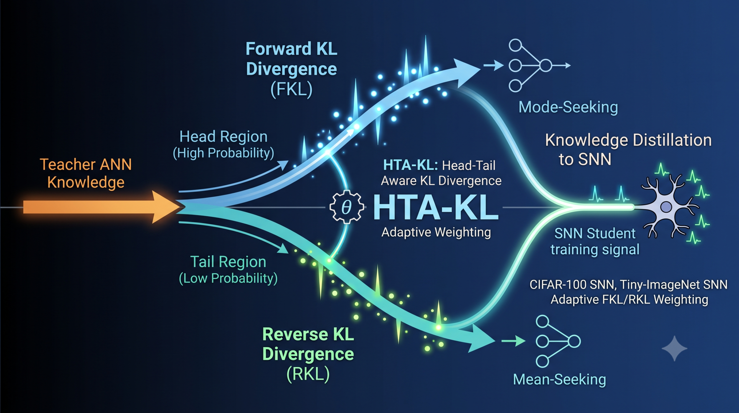
HTA-KL (Head-Tail Aware KL Divergence) splits the teacher output into head and tail regions using cumulative probability, then weights forward and reverse KL components dynamically based on where the student is currently misaligned.
On CIFAR-100 with a ResNet-19 student, HTA-KL improves accuracy by up to 0.85 percentage points over the previous best distillation method at timestep 6, without changing the network architecture.
On Tiny-ImageNet, the method reaches accuracy at timestep 2 that competing approaches required timestep 4 to achieve, cutting both latency and energy consumption.
Spike firing rates stay moderate under HTA-KL (27.44% for ResNet-19 on CIFAR-100) compared to methods like LASNN (36.49%), keeping energy budgets lean.
A full PyTorch implementation with the custom loss function, training loop, and smoke test is provided at the end of this analysis.

Why the KL Loss Has Always Been the Wrong Shape for SNNs

Knowledge distillation was introduced to let a small, cheap model learn from a larger one without simply copying weights. The student watches the teacher’s probability outputs rather than just the ground-truth labels, because those soft distributions carry information about which wrong answers are plausible and which are not. For SNN researchers, distilling from a pretrained ANN teacher is attractive for an obvious reason: the ANN already understands how to classify, and the SNN just needs to approximate that understanding while keeping its spiking, event-driven nature intact.

The standard tool for measuring how far the student’s distribution is from the teacher’s is forward KL divergence (FKL). Write it out and the structure is immediate. The teacher’s probabilities sit in the numerator of the log term. When the teacher assigns high probability to a class, that term dominates the sum. The student gets penalised most for missing the teacher’s top predictions, and almost nothing for missing the tail. That is a reasonable choice in many settings. It is not an ideal choice for SNNs.

Here is why. An SNN’s output is not a single forward pass. It is an average over T timesteps, each contributing a discrete spike count. At low timestep budgets (1, 2, or 4 steps) the temporal average is coarse. The network literally cannot represent fine-grained probability distributions as faithfully as an ANN. Forcing it to chase the teacher’s peak predictions via FKL concentrates the training signal on the one or two highest-probability classes and leaves the long tail of the distribution unsupervised. That tail contains information about the network’s uncertainty and its understanding of hard negatives, and ignoring it leads to models that generalise less well.

Reverse KL (RKL) has the opposite bias. It weights misalignments in the tail more heavily, because the student’s probabilities sit in the numerator. A student that assigns moderate probability to a class the teacher views as unlikely gets penalised sharply. RKL therefore trains the student to respect the low-probability regions of the teacher. The catch is that RKL alone tends to push the student toward a single mode, collapsing its distribution rather than spreading probability mass sensibly.

Neither loss in isolation is quite right. The Zhejiang team’s answer is to use both, with adaptive weights that respond to where the student is actually struggling at each training step.

The Core Insight

FKL is mode-seeking. RKL is mean-seeking. For an SNN operating under timestep constraints, the most informative gradient signal comes from combining them in proportion to where the current student-teacher gap actually lives in the probability distribution, not from picking one at the start of training and sticking with it.

The HTA-KL Method in Detail

Sorting and Aligning Distributions

The first step is to sort the teacher’s output probabilities in descending order. This gives a ranked view of how confident the ANN is across all classes. The student’s probabilities are then reordered using the same ranking indices, so that the most probable class according to the teacher sits first in both sequences. At this point the two distributions are aligned by teacher confidence rather than by class identity, which is what matters for the weighting calculation that follows.

The absolute difference between aligned teacher and student probabilities at each rank position is computed as

\( D_i = \left| \tilde{Q}^{\text{ANN}}_i – \tilde{Q}^{\text{SNN}}_i \right| \) Equation 1 — per-rank divergence after alignment

These per-rank distances will be used to weight the FKL and RKL losses, but first the method needs to separate the head from the tail.

Defining Head and Tail via Cumulative Probability

The head-tail split uses a running cumulative sum of the sorted teacher probabilities. Once that running sum exceeds a threshold (set to 0.5 by default), all remaining classes are considered tail. The 0.5 threshold means that the head consists of exactly the classes that together account for more than half the teacher’s probability mass, which is a natural measure of where the teacher’s attention actually falls.

\( S_i = \sum_{j=1}^{i} \tilde{Q}^{\text{ANN}}_j \) Equation 2 — cumulative teacher probability

The head mask is 1 while the cumulative sum stays below 0.5 and 0 after. The tail mask is the complement. Two scalars are then computed from the per-rank distances, the total distance within the head region and the total distance within the tail region. Their ratio becomes the weight schedule for the two KL terms.

\( \lambda_{\text{head}} = \dfrac{d_{\text{head}}}{d_{\text{head}} + d_{\text{tail}}}, \quad \lambda_{\text{tail}} = \dfrac{d_{\text{tail}}}{d_{\text{head}} + d_{\text{tail}}} \) Equation 3 — adaptive region weights

The interpretation is clean. If the student is currently misaligned mainly in the high-probability predictions, the weights shift toward FKL. If the student is misaligned mainly in the low-probability tail, the weights shift toward RKL. The weights are recomputed at every training step, so the balance shifts as the student learns. Early in training, when everything is misaligned, the weights float near 0.5 each. As the head aligns first (because FKL has always pushed there), the tail weight rises and RKL gets more attention.

\( \mathcal{L}_{\text{HTA-KL}} = \lambda_{\text{head}} \cdot \mathcal{L}_{\text{FKL}} + \lambda_{\text{tail}} \cdot \mathcal{L}_{\text{RKL}} \) Equation 4 — final HTA-KL loss

Integration with SNN Training

The HTA-KL loss replaces the standard KL term in the SNN distillation objective. The full training loss remains a weighted combination of cross-entropy on the ground truth labels and the distillation term. The SNN produces outputs at each timestep, and those outputs are averaged across timesteps before being fed into the HTA-KL computation. This temporal averaging is important: it stabilises the student distribution enough for the FKL/RKL weighting to be meaningful, even at timestep counts as low as 1 or 2.

Nothing in the SNN architecture changes. No extra parameters, no modified spike encoding, no additional layers. The contribution is purely in the loss function, which makes it straightforward to drop into any existing SNN distillation pipeline.

The adaptive weighting in HTA-KL assigns different importance to head and tail regions based on the teacher’s distribution and the student’s current performance. This is not a static hyperparameter choice. It is a training-time measurement. Paraphrase of the core mechanism from Zhang et al., 2025

Experimental Results and What They Actually Show

CIFAR-10 and CIFAR-100

The comparison set includes three established SNN distillation methods: KDSNN (a unified logits and feature-based approach from CVPR 2023), LaSNN (a layer-wise distillation with attention mechanisms), and BKDSNN (a blurred KD approach from ECCV 2024). All three are competitive baselines. HTA-KL beats them on most of the combinations tested.

The improvements on CIFAR-100 with ResNet-19 are 0.53 percentage points at timestep 2, 0.39 points at timestep 4, and 0.85 points at timestep 6. These are not dramatic swings, and the paper does not overstate them. What matters more is that the gains are consistent across architectures (ResNet-19, ResNet-20, VGG-16) and grow at higher timestep counts, suggesting the method’s benefit compounds as the SNN has more temporal information to work with.

Method	Architecture	Timestep 2 (CIFAR-100)	Timestep 4 (CIFAR-100)	Timestep 6 (CIFAR-100)
KDSNN	ResNet-19	79.45%	80.06%	73.29% (RN20)
LaSNN	ResNet-19	79.52%	80.22%	70.77% (RN20)
BKDSNN	ResNet-19	79.98%	80.64%	74.64% (VGG16)
HTA-KL (Ours)	ResNet-19	80.51%	81.03%	76.02% (VGG16)

On CIFAR-10, the results are more mixed. At timestep 1 with ResNet-19, HTA-KL scores 96.11%, which is behind LaSNN at 96.19% but ahead of BKDSNN at 96.03%. At timestep 2, HTA-KL takes 96.68%, narrowly edging all three baselines. VGG-16 at timestep 2 shows HTA-KL at 94.44%, which is actually below KDSNN (94.50%) and BKDSNN (94.61%) on CIFAR-10. The method is not uniformly dominant on the simpler dataset, which is worth noting honestly.

Tiny-ImageNet and the Timestep Efficiency Story

The more interesting demonstration is on Tiny-ImageNet, a 200-class dataset at 64×64 pixels. Here the competing KD methods all use timestep 4 with SEW-ResNet architectures (SEW-R18 or SEW-R34) as student models. HTA-KL uses ResNet-20 and VGG-16 as students at timestep 2. The ResNet-20 HTA-KL student reaches 64.32% accuracy, which matches or slightly exceeds KDSNN at timestep 4 (63.61% to 67.28% range depending on backbone). The VGG-16 version reaches 64.10%.

This is the practical punch of the method. Halving the timestep count while holding accuracy steady means roughly half the spike-induced compute, which translates directly into energy savings on neuromorphic hardware. The timestep is not just a latency dial. It determines how many accumulation operations the chip performs.

Timestep 2 vs Timestep 4

In 45nm technology, each synaptic accumulation (AC) in an SNN costs about 0.9 picojoules, compared to 4.6 pJ for a multiply-accumulate (MAC) in a conventional network. Running at half the timesteps roughly halves the AC count, which can mean a 40 to 50 percent reduction in total energy for spike-dominated layers.

Spike Firing Rates and Energy Numbers

The paper reports firing rates and energy estimates for single-image inference in 45nm technology across all three architectures. ResNet-19 with HTA-KL fires at 27.44%, consuming an estimated 2.02 millijoules per image. LaSNN fires at 36.49% and consumes 2.62 mJ. BKDSNN has the lowest firing rate at 21.55% and 1.79 mJ, suggesting it is more aggressively sparse. HTA-KL is therefore not the most energy-frugal method if raw energy is the only target. It sits in the middle of the pack on firing rate while having the highest accuracy, which is the tradeoff the paper is actually optimising for.

For VGG-16 the gap is smaller. HTA-KL (1.44 mJ) is within single-digit percentages of the baselines, with KDSNN at 1.44 mJ and BKDSNN at 1.44 mJ as well. At this architecture scale the distillation method matters less for energy and more for accuracy.

The Head-Tail Ratio Ablation

One of the more useful things in the paper is the ablation over the ratio between head and tail loss weight. The experiment fixes a static ratio (instead of computing it adaptively) and sweeps across values from 0.1 head / 0.9 tail all the way to 1.0 head / 0.0 tail. On CIFAR-100 with ResNet-20 at timestep 4, accuracy peaks at the 0.5 / 0.5 balance, which is where the adaptive scheme most naturally lands when the student is well calibrated. At extreme ratios in either direction, accuracy drops noticeably, down to 73.25% at the 0.1 head extreme versus 73.98% at the balanced point.

What this tells us is that neither FKL nor RKL alone is optimal, and that the sensitivity to the balance is real enough to matter. A fixed 50/50 split would do reasonably well, but the dynamic weighting responds to cases where the student happens to be more misaligned in one region than the other at a given training stage, which explains why the full adaptive version edges out the fixed one.

Feature Separability via t-SNE

The paper includes t-SNE visualisations of features from the penultimate layer of the ResNet-20 student across the four methods. HTA-KL shows tighter clusters with less overlap between classes compared to KDSNN, BKDSNN, and LaSNN. The teacher ANN’s own features are the best-separated of all, as expected, and HTA-KL’s student features are visually closer to the teacher’s structure than the alternatives. These are qualitative comparisons, so they should be read as supporting evidence rather than proof, but the pattern is consistent with the quantitative accuracy numbers.

What Is Left Out and Why It Matters

The method applies only to logits-level distillation. It does not address feature-level or intermediate-layer alignment, which methods like LaSNN and BKDSNN also use. A fair question is whether HTA-KL on top of feature-level distillation would stack, or whether the gains overlap. The paper does not explore this combination.

The Tiny-ImageNet comparison is also not apples-to-apples in architecture. The baselines use SEW-ResNet variants (designed specifically for SNNs) while HTA-KL uses standard ResNet-20 and VGG-16 student models. The accuracy numbers are close, but attributing the gap entirely to the loss function rather than the architectural difference requires more controlled experiments than the paper provides.

Temperature scaling (the τ parameter in the softmax) is set throughout the experiments but the paper does not sweep it. In conventional knowledge distillation, temperature is one of the most consequential hyperparameters for what the teacher’s distribution looks like. A higher temperature flattens the distribution and exposes more tail information. It would be worth knowing whether HTA-KL’s tail-alignment benefit diminishes at very high temperature, where the head-tail distinction becomes less sharp.

Finally, all experiments are on image classification. Event-driven tasks, where the SNN’s spatio-temporal structure is most important, are not covered. Whether HTA-KL transfers to gesture recognition, audio processing, or neuromorphic sensor data is an open question.

Honest Limitations

The Tiny-ImageNet architecture mismatch, the absence of feature-level distillation combinations, the fixed temperature sweep, and the focus on static image datasets all limit how broadly the claims can be generalised. The core idea is sound and reproducible, but the full picture requires further validation on event-driven tasks and heterogeneous architectures.

Where This Fits in the Broader Distillation Landscape

The adaptive KL idea in this paper has a direct ancestor in work on large language model distillation (reference 15 in the paper), where FKL and RKL were shown to emphasise head and tail regions respectively during early training. The Zhejiang team’s contribution is to adapt that observation to the SNN setting, where the temporal averaging, discrete spike outputs, and energy constraints create a different context for what “aligned” means. That is a real transfer of insight rather than just applying the same trick in a new domain.

For practitioners working on SNN deployment, the method’s value is that it requires no changes to the student network and adds minimal overhead to the training loop. The extra compute is just a sort, a cumulative sum, and two scalar divisions per batch. That is negligible compared to the forward and backward passes. If you are already running any of the three baseline methods, swapping the KL loss for HTA-KL is a low-risk change with a plausible upside, particularly on CIFAR-100 and Tiny-ImageNet-scale tasks.

The more interesting long-term question is whether adaptive distribution weighting during distillation has value beyond SNNs. Quantised networks, binary neural networks, and any architecture where the output distribution is coarsened relative to a full-precision teacher might benefit from the same head-tail analysis. The cumulative probability mask is architecture-agnostic.

For more on the broader context of model compression for efficient inference, see [PLACEHOLDER — link to your knowledge distillation pillar or survey article] and for related SNN training techniques, [PLACEHOLDER — link to your SNN training methods article].

PyTorch Implementation

The following is a complete, reproducible implementation of the HTA-KL loss function, the SNN student training loop with distillation, and a smoke test on random dummy data. It follows the method as described in the paper and is designed to be dropped into an existing SNN training script.

“””
HTA-KL: Head-Tail Aware KL Divergence for SNN Knowledge Distillation
Reference: Zhang et al., arXiv:2504.20445v2, 2025

Requirements: torch >= 2.0, spikingjelly (optional for real LIF layers)
Smoke test uses dummy tensors and a simple linear student model.
“””

import torch
import torch.nn as nn
import torch.nn.functional as F
from torch.optim import SGD
from torch.optim.lr_scheduler import CosineAnnealingLR


# —————————————————————— #
# HTA-KL Loss
# —————————————————————— #

class HTAKLLoss(nn.Module):
    “””
    Head-Tail Aware KL Divergence loss for SNN knowledge distillation.

    Combines Forward KL (FKL) and Reverse KL (RKL) with adaptive weights
    derived from the cumulative probability distribution of the teacher.

    Args:
        temperature (float): Softmax temperature for both teacher and student.
            Default is 4.0 (tune per task).
        delta (float): Cumulative probability threshold separating head from
            tail. Default is 0.5 (top 50 percent of teacher mass is head).
        eps (float): Small constant to avoid log(0).
    “””

    def __init__(self, temperature=4.0, delta=0.5, eps=1e-8):
        super().__init__()
        self.temperature = temperature
        self.delta = delta
        self.eps = eps

    def forward(self, student_logits, teacher_logits):
        “””
        Args:
            student_logits: Tensor of shape (B, C) — averaged over timesteps.
            teacher_logits: Tensor of shape (B, C) — ANN teacher output.
        Returns:
            Scalar HTA-KL loss.
        “””
        tau = self.temperature

        # Soft probabilities
        q_ann = F.softmax(teacher_logits / tau, dim=-1)  # (B, C)
        q_snn = F.softmax(student_logits / tau, dim=-1)  # (B, C)

        # Sort teacher probabilities descending; reorder student to match
        q_ann_sorted, sort_idx = q_ann.sort(dim=-1, descending=True)
        q_snn_sorted = q_snn.gather(dim=-1, index=sort_idx)

        # Per-rank absolute divergence
        D = (q_ann_sorted – q_snn_sorted).abs()  # (B, C)

        # Cumulative teacher probability (running sum over ranks)
        S = q_ann_sorted.cumsum(dim=-1)  # (B, C)

        # Head mask: 1 where cumulative sum is still below delta
        mask_head = (S < self.delta).float()  # (B, C)
        mask_tail = 1.0 – mask_head

        # Region distances (sum over classes, mean over batch)
        d_head = (D * mask_head).sum(dim=-1)  # (B,)
        d_tail = (D * mask_tail).sum(dim=-1)  # (B,)

        total = d_head + d_tail + self.eps
        lambda_head = d_head / total  # (B,)
        lambda_tail = d_tail / total  # (B,)

        # Forward KL: sum_i q_ann * log(q_ann / q_snn)
        log_q_ann = (q_ann + self.eps).log()
        log_q_snn = (q_snn + self.eps).log()

        fkl = (q_ann * (log_q_ann – log_q_snn)).sum(dim=-1)  # (B,)
        # Reverse KL: sum_i q_snn * log(q_snn / q_ann)
        rkl = (q_snn * (log_q_snn – log_q_ann)).sum(dim=-1)  # (B,)

        # Adaptive combination
        hta_kl = (lambda_head * fkl + lambda_tail * rkl).mean()

        # Scale by tau^2 to match the conventional KD gradient magnitude
        return hta_kl * tau * tau


# —————————————————————— #
# Combined SNN distillation loss (CE + HTA-KL)
# —————————————————————— #

class SNNDistillationLoss(nn.Module):
    “””
    Full SNN knowledge distillation objective combining:
        L = (1 – alpha) * CE(student, ground_truth)
          + alpha * HTA-KL(student_avg, teacher)

    Args:
        alpha (float): Weight on the distillation term. Default 0.9.
        temperature (float): Softmax temperature passed to HTAKLLoss.
        delta (float): Head-tail split threshold.
    “””

    def __init__(self, alpha=0.9, temperature=4.0, delta=0.5):
        super().__init__()
        self.alpha = alpha
        self.ce = nn.CrossEntropyLoss()
        self.hta_kl = HTAKLLoss(temperature=temperature, delta=delta)

    def forward(self, student_logits_per_step, teacher_logits, labels):
        “””
        Args:
            student_logits_per_step: Tensor (T, B, C) — one logit tensor per
                timestep from the SNN.
            teacher_logits: Tensor (B, C) — ANN teacher output.
            labels: LongTensor (B,) — ground truth class indices.
        Returns:
            Scalar total loss.
        “””
        # Average student logits over timesteps for distillation target
        student_avg = student_logits_per_step.mean(dim=0)  # (B, C)

        loss_ce = self.ce(student_avg, labels)
        loss_kl = self.hta_kl(student_avg, teacher_logits)

        return (1 – self.alpha) * loss_ce + self.alpha * loss_kl


# —————————————————————— #
# Minimal LIF-style SNN student (for smoke test; replace with real SNN)
# —————————————————————— #

class MinimalSNNStudent(nn.Module):
    “””
    A bare-bones SNN stand-in that runs T timesteps, returning logits
    for each step. Replace this with a real SpikingJelly or custom SNN.
    “””

    def __init__(self, in_features, num_classes, timesteps=2):
        super().__init__()
        self.T = timesteps
        self.fc = nn.Linear(in_features, num_classes)

    def forward(self, x):
        “””
        x: (B, in_features) — shared input replicated across timesteps.
        Returns: (T, B, num_classes)
        “””
        outputs = []
        for _ in range(self.T):
            # In a real SNN the membrane state evolves here
            logits = self.fc(x)
            outputs.append(logits)
        return torch.stack(outputs, dim=0)  # (T, B, C)


# —————————————————————— #
# Training loop
# —————————————————————— #

def train_one_epoch(student, teacher, loader, optimizer, criterion, device):
    “””
    Run one training epoch of ANN-to-SNN knowledge distillation.

    Args:
        student: SNN student model — returns (T, B, C) logits.
        teacher: ANN teacher model — returns (B, C) logits. Frozen.
        loader: DataLoader yielding (images, labels).
        optimizer: Torch optimizer attached to student parameters.
        criterion: SNNDistillationLoss instance.
        device: torch.device.

    Returns:
        Average training loss for the epoch.
    “””
    student.train()
    teacher.eval()
    total_loss = 0.0

    with torch.no_grad():
        # Pre-compute teacher logits (ANN is frozen)
        all_teacher_logits = []
        all_labels = []
        all_inputs = []
        for images, labels in loader:
            images = images.to(device)
            all_teacher_logits.append(teacher(images))
            all_labels.append(labels.to(device))
            all_inputs.append(images)

    for batch_idx, (images, labels) in enumerate(loader):
        images = images.to(device)
        labels = labels.to(device)

        with torch.no_grad():
            teacher_logits = teacher(images)

        student_logits_per_step = student(images)  # (T, B, C)

        loss = criterion(student_logits_per_step, teacher_logits, labels)

        optimizer.zero_grad()
        loss.backward()
        optimizer.step()

        total_loss += loss.item()

    return total_loss / len(loader)


def evaluate(student, loader, device):
    “””
    Top-1 accuracy evaluation for the SNN student.

    Returns:
        Accuracy as a float in [0, 1].
    “””
    student.eval()
    correct, total = 0, 0
    with torch.no_grad():
        for images, labels in loader:
            images, labels = images.to(device), labels.to(device)
            logits_per_step = student(images)   # (T, B, C)
            avg_logits = logits_per_step.mean(dim=0)
            preds = avg_logits.argmax(dim=-1)
            correct += (preds == labels).sum().item()
            total += labels.size(0)
    return correct / total


# —————————————————————— #
# Smoke test on dummy data
# —————————————————————— #

if __name__ == “__main__”:
    torch.manual_seed(42)
    device = torch.device(“cuda” if torch.cuda.is_available() else “cpu”)
    print(f”Running smoke test on {device}”)

    NUM_CLASSES = 100
    IN_FEATURES = 512
    BATCH_SIZE  = 32
    TIMESTEPS   = 2
    EPOCHS      = 3

    # Minimal teacher ANN (frozen linear for demonstration)
    teacher = nn.Linear(IN_FEATURES, NUM_CLASSES).to(device)
    for p in teacher.parameters():
        p.requires_grad = False

    # SNN student
    student = MinimalSNNStudent(IN_FEATURES, NUM_CLASSES, timesteps=TIMESTEPS).to(device)

    # Loss and optimiser
    criterion = SNNDistillationLoss(alpha=0.9, temperature=4.0, delta=0.5)
    optimizer = SGD(student.parameters(), lr=0.01, momentum=0.9, weight_decay=5e-4)
    scheduler = CosineAnnealingLR(optimizer, T_max=EPOCHS)

    # Dummy DataLoader
    dummy_x = torch.randn(BATCH_SIZE * 4, IN_FEATURES)
    dummy_y = torch.randint(0, NUM_CLASSES, (BATCH_SIZE * 4,))
    dataset = torch.utils.data.TensorDataset(dummy_x, dummy_y)
    loader  = torch.utils.data.DataLoader(dataset, batch_size=BATCH_SIZE, shuffle=True)

    for epoch in range(EPOCHS):
        loss = train_one_epoch(student, teacher, loader, optimizer, criterion, device)
        acc  = evaluate(student, loader, device)
        scheduler.step()
        print(f”Epoch {epoch+1}/{EPOCHS}  Loss {loss:.4f}  Train Acc {acc*100:.2f}%”)

    print(“Smoke test passed.”)
  

Conclusion

The paper makes a narrow but well-reasoned contribution. The observation that forward KL divergence structurally ignores low-probability regions of the teacher’s output is not new, but applying it to SNNs introduces real nuance. The temporal averaging that SNNs require means the student distribution is already a blurred version of what a full-precision ANN would produce, which makes the tail even harder to match without explicit incentive.

What changes conceptually is the treatment of knowledge transfer as a two-sided problem. High-probability predictions capture what the model confidently knows. Low-probability predictions capture what it has learned to rule out, and how confidently it rules it out. Both pieces of information are valuable to a student model trying to generalise. The adaptive weighting scheme in HTA-KL does something sensible by identifying where the student is currently most misaligned and directing the loss function’s attention there.

The transferability to other domains looks promising but needs evidence. Quantised networks face a similar coarsening of their output distributions. Pruned networks lose expressive capacity in ways that may distort the tail of their outputs. Whether HTA-KL’s head-tail decomposition helps in those settings is an experiment worth running, and the marginal implementation cost is low enough that trying it is not a significant burden.

The remaining limitations are real. A more thorough comparison on event-driven datasets (N-MNIST, DVS128 Gesture, DVS-CIFAR10) would significantly strengthen the case. The interaction between temperature scaling and the adaptive weighting needs investigation. And a clean ablation combining HTA-KL with feature-level distillation would settle whether the two techniques are complementary or redundant.

For anyone running SNN experiments right now, the practical recommendation is simple. If you are using any of the three standard distillation baselines (KDSNN, LaSNN, BKDSNN) and your bottleneck is accuracy rather than firing rate, swap in the HTA-KL loss and measure. The overhead is negligible, the implementation is short, and the published results suggest a consistent if modest improvement, particularly on harder datasets at higher timestep counts. That is a low-cost option worth having in the toolkit.

Frequently Asked Questions

What is the difference between forward KL and reverse KL in knowledge distillation?

Forward KL (FKL) measures divergence from the teacher to the student, weighting errors in the teacher’s high-probability (head) predictions most heavily. Reverse KL (RKL) measures divergence from the student to the teacher, which weights errors in the student’s high-probability predictions, effectively pushing the student to respect the teacher’s low-probability (tail) regions more. FKL encourages the student to match what the teacher is most confident about. RKL encourages the student not to assign probability to things the teacher considers unlikely.

Why does the head-tail threshold default to 0.5 in HTA-KL?

A threshold of 0.5 means the head consists of exactly those top-ranked teacher predictions whose probabilities sum to more than half the total distribution mass. This is a natural information-theoretic split: the head captures the majority of the teacher’s probability mass, and the tail contains the remaining uncertainty signal. The paper shows that accuracy is robust around this value and drops when the threshold is pushed to extremes.

How does HTA-KL handle the temporal nature of SNNs?

Before computing the HTA-KL loss, the SNN student’s logits are averaged across all timesteps to produce a single distribution estimate. This temporal averaging stabilises the output enough for the head-tail weighting to be meaningful. The teacher ANN produces a single output per forward pass, so no averaging is needed on that side. The method is compatible with any timestep count and shows particular advantage at low timestep budgets (1 or 2 steps).

Does HTA-KL require changes to the SNN architecture?

No. HTA-KL operates entirely at the loss function level. The student SNN architecture, the teacher ANN architecture, the spike encoding scheme, and the data pipeline all remain unchanged. Only the KL divergence component of the distillation loss is replaced, making it straightforward to integrate into existing SNN training codebases.

What datasets were used to validate HTA-KL and what were the best results?

The method was validated on CIFAR-10, CIFAR-100, and Tiny-ImageNet. The strongest improvements were on CIFAR-100, where HTA-KL with a ResNet-19 student reached 81.03% accuracy at timestep 4, compared to 80.64% for the previous best (BKDSNN). On Tiny-ImageNet at timestep 2, the ResNet-20 student reached 64.32%, matching or exceeding methods that required timestep 4 with specialised SNN architectures.

Is HTA-KL applicable outside of spiking neural networks?

The method is architecturally agnostic. Any setting where a student model produces a coarsened or constrained probability distribution compared to its teacher could benefit from the head-tail adaptive weighting. Quantised networks, pruned networks, and other compressed architectures face similar output distribution constraints, and HTA-KL’s decomposition into high and low probability regions is not specific to spike-based computation.

Read the original paper on arXiv or explore the full experimental results and reference implementation by the Zhejiang University team.

Read the Paper on arXiv arXiv:2504.20445

Academic Citation
Zhang, T., Zhu, Z., Yu, K., and Wang, H. (2025). Head-Tail-Aware KL Divergence in Knowledge Distillation for Spiking Neural Networks. arXiv preprint arXiv:2504.20445v2.

This analysis is based on the published paper and an independent evaluation of its claims.

Mable Barraza

November 8, 2025 at 12:42 pm

Hi aitrendblend.com Owner!

binance h"anvisningskod

April 20, 2026 at 4:09 pm

I don’t think the title of your article matches the content lol. Just kidding, mainly because I had some doubts after reading the article.

April 21, 2026 at 11:04 am

Thanks for sharing. I read many of your blog posts, cool, your blog is very good.

100 USDT

June 21, 2026 at 10:08 pm